HAL Id: hal-01595236
https://hal.archives-ouvertes.fr/hal-01595236
Submitted on 26 Sep 2017HAL is a multi-disciplinary open access archive for the deposit and dissemination of sci-entific research documents, whether they are pub-lished or not. The documents may come from teaching and research institutions in France or abroad, or from public or private research centers.
L’archive ouverte pluridisciplinaire HAL, est destinée au dépôt et à la diffusion de documents scientifiques de niveau recherche, publiés ou non, émanant des établissements d’enseignement et de recherche français ou étrangers, des laboratoires publics ou privés.
Estimation of available water capacity components of
two-layered soils using crop model inversion: Effect of
crop type and water regime
Sreelash Krishnan Kutty, Samuel Buis, M. Sekhar, Laurent Ruiz, Sat Kumar
Tomer, Martine Guerif
To cite this version:
Sreelash Krishnan Kutty, Samuel Buis, M. Sekhar, Laurent Ruiz, Sat Kumar Tomer, et al.. Es-timation of available water capacity components of two-layered soils using crop model inversion: Effect of crop type and water regime. Journal of Hydrology, Elsevier, 2017, 546, pp.166-178. �10.1016/j.jhydrol.2016.12.049�. �hal-01595236�
Accepted Manuscript
Research papers
Estimation of available water capacity components of two-layered soils using crop model inversion: Effect of crop type and water regime
K. Sreelash, Samuel Buis, M. Sekhar, Laurent Ruiz, Sat Kumar Tomer, Martine Guerif
PII: S0022-1694(16)30846-0
DOI: http://dx.doi.org/10.1016/j.jhydrol.2016.12.049
Reference: HYDROL 21728
To appear in: Journal of Hydrology Received Date: 21 March 2016 Revised Date: 22 December 2016 Accepted Date: 24 December 2016
Please cite this article as: Sreelash, K., Buis, S., Sekhar, M., Ruiz, L., Kumar Tomer, S., Guerif, M., Estimation of available water capacity components of two-layered soils using crop model inversion: Effect of crop type and water regime, Journal of Hydrology (2016), doi: http://dx.doi.org/10.1016/j.jhydrol.2016.12.049
This is a PDF file of an unedited manuscript that has been accepted for publication. As a service to our customers we are providing this early version of the manuscript. The manuscript will undergo copyediting, typesetting, and review of the resulting proof before it is published in its final form. Please note that during the production process errors may be discovered which could affect the content, and all legal disclaimers that apply to the journal pertain.
1
Estimation of available water capacity components of two-layered soils using crop model
inversion: Effect of crop type and water regime
K. Sreelash a,b,c,d, Samuel Buis a,b,*, M. Sekhar c,e,Laurent Ruiz c,e,f,g, Sat Kumar Tomerc,e,h,
Martine Guerif a,b.
a
INRA, EMMAH, UMR 1114, F-84 914 Avignon, France
b
UAPV, EMMAH, UMR 1114, F-84 914 Avignon, France
c
Indo-French Cell for Water Sciences, Indian Institute of Science, IRD, Bangalore, India
d
National Centre for Earth Science Studies, Thiruvananthapuram, India
e
Department of Civil Engineering, Indian Institute of Science, Bangalore, India
f
UMR SAS, INRA, AGROCAMPUS OUEST, 35000 Rennes, France
g
GET, CNRS, UPS, IRD, CNES, 31400 Toulouse, France
h
Aapah Innovations Private Limited, Hyderabad 500 032, India
*Corresponding author: samuel.buis@paca.inra.fr
Abstract
Characterization of the soil water reservoir is critical for understanding the interactions
between crops and their environment and the impacts of land use and environmental changes
on the hydrology of agricultural catchments especially in tropical context. Recent studies have
shown that inversion of crop models is a powerful tool for retrieving information on root zone
properties. Increasing availability of remotely sensed soil and vegetation observations makes
it well suited for large scale applications. The potential of this methodology has however
2
suggested that the quality of estimation of soil hydraulic properties may vary depending on
agro-environmental situations. The objective of this study was to evaluate this approach on an
extensive field experiment. The dataset covered four crops (sunflower, sorghum, turmeric,
maize) grown on different soils and several years in South India. The components of AWC
(available water capacity) namely soil water content at field capacity and wilting point, and
soil depth of two-layered soils were estimated by inversion of the crop model STICS with the
GLUE (generalized likelihood uncertainty estimation) approach using observations of surface
soil moisture (SSM; typically from 0 to 10 cm deep) and leaf area index (LAI), which are
attainable from radar remote sensing in tropical regions with frequent cloudy conditions. The
results showed that the quality of parameter estimation largely depends on the hydric regime
and its interaction with crop type. A mean relative absolute error of 5% for field capacity of
surface layer, 10% for field capacity of root zone, 15% for wilting point of surface layer and
root zone, and 20% for soil depth can be obtained in favorable conditions. A few observations
of SSM (during wet and dry soil moisture periods) and LAI (within water stress periods) were
sufficient to significantly improve the estimation of AWC components. These results show
the potential of crop model inversion for estimating the AWC components of two-layered
soils and may guide the sampling of representative years and fields to use this technique for
mapping soil properties that are relevant for distributed hydrological modelling.
Keywords: Soil Hydraulic Properties ; Available Water Capacity ; STICS ; soil water content
; GLUE ; Inverse modelling
1.0 Introduction
The capacity of the soil to store water available for plants, generally referred as available
water capacity (AWC) is a key parameter for modelling the catchment-scale water balance. In
3
rainfall, recharge to groundwater is difficult to estimate from vadose-zone water balance (De
Vries et Simmers, 2002) and it is particularly sensitive to the size of the soil water storage
(Anuraga et al., 2006 ; Sreelash et al. 2013). Therefore, accurate estimates of AWC and its
spatial variability at the catchment scale are needed to improve the sustainable management of
groundwater resources. The increasing availability of high frequency and high resolution
remote-sensing data now allows retrieving precise soil hydraulic properties maps of the top
few centimeters of the soil (Montzka et al., 2011) but estimating AWC of the entire root zone
at the catchment scale remains a challenge.
AWC depends on soil hydraulic properties (SHPs), soil depth and plant rooting
characteristics. It may be defined from different point of view - pedologists, soil scientists,
ecophysiologists - with different approaches and different levels of complexity, considering
one or several layers corresponding to pedological horizons. A common definition of the
AWC is the difference between the soil water content at field capacity and wilting point
(Bruand et al., 2003). Those parameters can be determined in the field, which minimize soil
disturbance or in the laboratory which requires soil sampling and sample preparation that
could distort the soil sample and increase the margins of errors. All methods are highly
time-consuming and expensive (Steele-Dunne et al., 2010; Botula et al., 2012). Therefore, it is
impractical to use them to obtain soil properties for catchments larger than a few hectares. For
larger areas SHPs are generally estimated from soil characteristics that are easily available
from soil maps (mainly textural properties) using pedotransfer functions (PTFs). However,
PTFs are often site-specific and may lead to crude estimates of SHPs with large uncertainties
when extrapolated over large areas (Vereecken et al., 1989, 1990, Wösten, 2001, Stump et al.,
2009) or beyond the specific context (geomorphic regions or soil type) under which they are
developed (McBartney et al., 2002). A more recent technique is Digital Soil Mapping (DSM)
4
inference systems (Lagacherie and McBratney, 2007). DSM makes an extensive use of
technological and computational advances such as remote sensing and geostatistics for
producing digital maps of soil types and soil properties (Lagacherie et al., 2008; Vaysse and
Lagacherie, 2015). However, approaches based on DSM estimates basic soil properties such
as soil texture, bulk density, pH etc. and still rely on PTFs to translate them into more
functional properties (McBratney et al., 2003). They are thus also limited by the quality of the
PTFs and their adequacy to the studied situation.
As AWC components are important parameters for hydrological models, model inversion is
another alternative for retrieving them. The principle is to use in situ or remotely sensed
observations corresponding to model outputs strongly linked with AWC components to
estimate them using parameter estimation or data assimilation methods. Such approach has
been carried out in several studies for estimating SHPs and soils depth using various types of
models: hydrological models (Ritter et al., 2003; Ines and Mohanty, 2008;
Charoenhirunyingyos et al., 2011), crop models (Guérif at al., 2006, Varella et al., 2010a,
2010b; Sreelash et al., 2012), Land Surface Models (Bandara et al., 2013, 2014 and 2015) or
SVAT (soil vegetation atmosphere transfer) models (Jhorar et al, 2002, 2004). Several studies
have shown that SHPs of vertically homogeneous soils can be estimated through model
inversion using surface soil moisture (see for example Montzka et al., 2011; Nagarajan et al.,
2011). For multi-layered soils, profile soil moisture observations allow assessing SHPs (Ritter
et al., 2003; Braga and Jones, 2004; Wohling et al., 2010; Li et al., 2011) but this requires
large experimental settings which limits its spatial application. On the other hand, using only
surface soil moisture measurements that can be spatially available from remote sensing, is not
sufficient to provide unique and physically reasonable estimates of hydraulic properties for
multi-layered soils through model inversion (Vereecken et al., 2008; Ines and Mohanty 2008;
5
between layers (Montzka et al., 2011), except in some particular situations (Shin et al., 2012;
Bandara et al., 2013). Shin et al. (2012) also reported that the weakness of hydrological
models in simulating plant root activities in the root zone results in relatively larger errors in
the estimation of SHPs in crop land as compared to bare soil. As crop lands represent a large
contribution to hydrologic processes within agricultural catchments, precise knowledge of
AWC components is critical for managing water resources to maintain agricultural
production. The known projections of climate change make this objective even more
essential.
Recently, crop model inversion has been proposed by several authors to retrieve AWC
components (Guérif et al., 2006; Varella et al., 2010a, 2010b; Sreelash et al., 2012). The
main interest of using of crop models for retrieving AWC components in crop lands is that
they are more efficient than hydrological models, Land Surface Models or SVAT models in
describing the specificity of crop behavior with regards to water processes (effect of crop type
on rooting system characteristics and water needs, effect of crop management practices on the
water balance). This is partly because they account AWC components impacts not only on the
soil water balance, but also on the coupled carbon and nitrogen cycling (Ruget et al., 2002;
Satti et al., 2004; Breda et al., 2006). The increasing availability of high frequency and high
resolution vegetation and soil moisture data from remote sensing makes crop model inversion
approach a potentially powerful tool for spatial applications, especially for parameterizing
catchment-scale hydrological models.
However, accuracy of the parameter estimates strongly depends on environmental conditions
such as climate and crop type (Varella et al., 2010b). Charoenhirunyingyos et al. (2011) and
Sreelash et al. (2012) show that combining surface soil moisture and vegetation measurements
6
substantially parameter estimation. However, these conclusions are based on synthetic
experiments or very limited field datasets. In fact, few studies based on field data have been
carried out to evaluate the potential of model inversion methods for estimating AWC
components on multi-layered soils with observations potentially accessible from remote
sensing and this problem is still considered as challenging (Mohanty 2013).
In this paper, we used an extensive field dataset from a tropical agricultural catchment in
South India involving four types of crops across 3 years. The objectives are:
(i) to analyze the potential of model inversion methods for estimating AWC components
(water content at field capacity and wilting point, soil depth) on two-layered soils with
observations potentially accessible from remote sensing on a large set of field situations; and
(ii) to investigate the influence of the crop type and water regimes experienced by the crops
on the accuracy of these estimations.
2.0 Materials and Methods
2.1 Site information
The experimental catchment of Berambadi (84 km2) is located in the Kabini river basin in
South India (AMBHAS Site, www.ambhas.com, long term environmental observatory BVET
http://bvet.obs-mip.fr; Braun et al., 2009; Ruiz et al., 2010; Violette et al., 2010). It is
intensively used for agro-hydrological, remote sensing and hydrological investigations
(Kumar et al., 2009). The land is used for agriculture and the crops are mostly rainfed or
irrigated with groundwater. We used a total of 60 crop/soil/climate situations covering 4 crops
across 3 years from May 2011 to Dec 2013 and 42 agricultural plots each approximately 1 ha
in size, monitored for soil moisture and crop growth. Among them, 15 crop/soil/climate
7
2.4). The inversions were performed on 45 crop/soil/climate situations from 33 plots. The
results presented in the following will only concern the situations/plots used for the
inversions.
The 4 crops studied have distinct characteristics (Table 1). Turmeric is an irrigated 8 months
crop (May to December) while the 3 others are rainfed crops grown over 4 months (May to
August for sunflower and sorghum and September to December for maize).
< Table 1 here please >
The climate is tropical semi-arid, dominated by south-west monsoon with a mean annual
rainfall of 800 mm (coefficient of variation 0.28), and an annual Potential Evapotranspiration
(PET Penman Method, Penman, 1948) of 1100 mm (coefficient of variation 0.05), computed
over 2005-2015. Daily records of air humidity, wind velocity, maximum and minimum air
temperatures, precipitation and global radiation were obtained from an automatic weather
station (CIMEL, type ENERCO 407 AVKP) and a meteorological flux tower (Astra
Microwave, India) located in the study area. Measurements from the closest station were
considered for each plot.
< Table 2 here please >
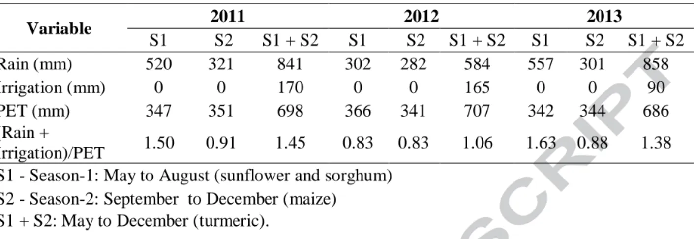
For the study period, the amount and distribution of rainfall and (Rain+ Irrigation)/PET ratio
varied across years and cropping seasons (Table 2). This led to a varying degree of crop water
stress experienced by the crops. 2012 was relatively dry as compared to 2011 and 2013 which can be classified as “normal years”.
8
Information on management activities such as date and dose of sowing, fertilizing, irrigation
and date of harvest were obtained during field visits. Sowing dates (expressed as day of the
year) vary between 130 to 150 for Sunflower and Sorghum, between 110 and 124 for turmeric
and between 250 and 262 for maize. Fertilizer is applied once at the beginning of the season,
the quantity varying between 20 to 30 kg.N/ha for sunflower, 30 to 50 kg.N/ha for sorghum,
100 to 200 kg.N/ha for turmeric and 25 to 50 kg.N/ha for maize.
LAI was measured using a Portable Leaf Area meter CI – 202 (CID Bioscience) and a
LAI-2000 Plant Canopy Analyzer (LI-COR) every 10 days in 2011 and 2012, and every 20 days in
2013 concurrently with soil moisture measurements (see next section). Three measurements
of LAI were taken in one representative sample area of 2 m2 and the mean value was used as
representative of the plot.
< Figure 1 here please >
Time series of LAI (Fig. 1) obtained by interpolation of the measurements using a parametric
growth curve approach (Baret, 1986) revealed a large variability resulting mainly from
interactions between crop, climate and soil type. It provides the basis for the determination of
root zone soil water content properties from crop model inversion.
2.3 Soils: pedology, soil moisture measurements, reference AWC parameters values
Soils in the studied area are roughly classified as red soils (Alfisols, FAO) or black soils
(Vertisols, FAO). According to the 1:50,000 scale soil map of the area prepared by Karnataka
State Remote Sensing Application Center (KSRSAC), six categories are considered based on
the particle size distribution of the top layer: Clay and Clay Loam for vertisols, Gravelly
9
is the major soil class, covering 50 % of the area. The soil is gravelly sandy loam at the hill
slopes, sandy loam and sandy clay loam in the plains and clay loam and clay soil in the valley.
Surface soil moisture (SSM; typically from 0 to 10 cm deep) used for model inversion was measured using Theta Probe Soil moisture sensor – ML2x (Delta-T devices, sampling
volume: 2.5 cm diameter, 6 cm long) and the mean of 3 measurements used as representative
of each field plot. Additionally three soil samples per plot were collected for gravimetric soil
moisture measurements. Theta Probe devices were calibrated twice a year using the
gravimetric measurements: once during period of low soil moisture (before the start of the
cropping season) and other during period of high soil moisture (during or at the end of the
first cropping season). Profiles of soil moisture - used to determine in situ soil hydraulic
properties – were also measured using soil moisture sensors (Trime-FM TDR, IMKO
Micromodultechnik GmbH, sampling volume: 15 cm diameter, 18 cm long). The
measurements were made at an increment of 10 cm from surface up to 1 m depth for shallow
soils and up to a depth of 2 m for deeper soils. Both surface and profile soil moisture were
measured throughout the year at a frequency of 10 days in 2011 to 2012 and 20 days in 2013.
To capture the extreme values of soil moisture in both dry and wet conditions, surface and
profile soil moisture were measured daily for a 30 day period once in October 2011 and once
in August 2013.
< Table 3 here please >
To compare the estimated values of soil properties retrieved from model inversion to ‘observed values’, water content at field capacity (θFC), wilting point (θWP) and soil depth (DL)
were determined from in situ measurements on the monitored plots (Table 3). As proposed
by Hunt et al. (2009) and Martinez-Fernandez et al. (2015), θFC and θWP were inferred from
10
moisture in the growing season, while discarding soil moisture data immediately after a
rainfall event (or irrigation event), and θWP as the ‘5th percentile of the minimum values’ of
soil moisture in the growing season. Our time series of soil moisture exhibited alternate
wetting and drying cycles, thus capturing both maximum and minimum soil water content.
Bulk density was determined as the ratio of volumetric soil moisture (from TDR
measurements) to gravimetric soil moisture (measured on soil samples). The depth of soil
layers was determined by soil augering. The depth of soil from surface to weathering zone
varied from 70 cm to 150 cm and was independent of the soil type.
2.4 Model and Parameters
The STICS crop model (Brisson et al., 1998; Coucheney et al., 2015) is a daily time-step
model which simulates the functioning of a soil-crop system over a single or several
successive crop cycles. It has been successfully used for spatial applications and coupled with
hydrological models at the catchment scale (Beaujouan et al., 2001). The upper boundary
conditions are governed by standard climatic variables (radiation, maximum and minimum air
temperatures, rainfall, potential evapotranspiration) and the lower boundary condition is the
soil/sub-soil interface. We used the Penman method to calculate potential evapotranspiration
(PET; Penman, 1948). Crops are described by their LAI, above-ground biomass and nitrogen
content and the number and biomass of harvested organs. The main processes described are
carbon assimilation and allocation to different organs and water and nitrogen balances (for
detailed description, see Brisson et al, 1998, 2008).
The different components of actual evapotranspiration (ET) are calculated from the potential
evapotranspiration: soil evaporation (Es), plant transpiration (Tp) and evaporation from the
water intercepted by the foliage that contributes to reducing the evaporative demand at the
11
evaporates at the potential rate, and a second stage where evaporation is lower and decreases
according to climate and type of soil. Crop water requirements (or maximum transpirat ion)
are determined according to a crop coefficient approach which is well adapted to the crops
considered herein (Brisson, 1998, 2008). The actual plant transpiration Tp is based on the
water physically available in the soil and the capacity of the plant to extract it, due to its root
characteristics, corresponding to the concept of AWC (amount of water between field
capacity FC and wilting point WP). The ratio of actual transpiration to maximal transpiration,
is a bilinear function of the amount of water available in the rooting zone (with a minimum
value of 0 when the soi1 water content is equal to WP and a maximum value equal to (FC -WP)). The soil water content regarded as being the threshold between the maximal
transpiration stage and the reduced transpiration stage depends on root density, stomatal
functioning of the plant and climatic demand. Water stress indices are derived from those
calculations and affect different components of plant growth.
The soil is considered as a reservoir and is defined as a succession of up to five homogeneous
layers characterized each by its retention capacity characteristics (FC and WP, bulk density
and thickness). Water transfer downwards in the soil microporosity is simulated on a
one-dimensional regular mesh discretized per 1cm step with a functional reservoir type model
according to the tipping bucket concept. Incoming water fills the layers by downward flow, assuming that the upper limit of each single reservoir corresponds to the layer’s field capacity. The STICS model contains about 200 input parameters which are related to the characteristics
of the plant, soil and crop management activities. The plant parameters for sunflower,
sorghum, turmeric and maize related to leaf growth, biomass, yield, and root growth were
calibrated with the OptimiSTICS software (Buis et al., 2011), using all the available data on a
12
model, the crop specific parameters can be assumed constant for the given crop for the study
area. The parameters related to the agricultural practices (sowing dates, fertilization dates and
doses, irrigation dates and doses and harvest dates) were set in accordance with the
information collected from farmers.
< Table 4 here please >
In order to reduce the number of soil parameters to be potentially estimated, we adopted the
simplified representation of the soil proposed by Varella et al. (2010a): a surface layer and a
second layer mainly representing the root zone. The first layer depth was set at 10 cm which
is compatible both with our field measurements of SSM and the order of magnitude of SSM
retrievals from radar remote sensing (Jackson et al., 1995, Baghdadi et al, 2006) for further
applications at larger scale. Here we considered only the permanent soil properties related to
water storage and transfers in the soil and restricted the estimation to five parameters: soil
moisture at field capacity (θFC) and wilting point (θWP) of both layers and thickness of the
second layer (DL2) (Table 4). These parameters describe the maximum AWC (expressed in
mm) of each layer which determines maximum water storage and available water for plant
uptake as follow:
(1)
where BD is the bulk density (g/cm3) and is the thickness (cm) of the layer.
These parameters influence also other processes such as soil evaporation, carbon and nitrogen
cycle in the soil (Brisson et al, 2008). They are involved separately in some of these processes
which bring independent constraints for their estimation. The soil input parameters
non-estimated in the inversion process were obtained from local soil maps, soil experiments and
13
2.5 Inversion method
Generalized Likelihood Uncertainty Estimation (GLUE) approach is an informal Bayesian
method using prior information of parameter values for estimating model parameters (Beven
and Binley, 1992; Makowski et al., 2002). Based on Monte Carlo simulation, GLUE
transforms the problem of searching an optimal parameter set into searching sets of parameter
values which would produce reliable simulations of the variables of interest (Aronica et al.,
2002). GLUE based approaches have been successfully applied to hydrological models (e.g.
Li et al., 2010) and dynamic crop models (Makowski, 2004 ; Guérif et al., 2006 ; Varella et
al., 2010a, 2010b ; Sreelash et al., 2012).
Sets of parameters values are randomly chosen in a prior distribution representing the
potential parameter space. These sets are then used in model simulations, which produce
multiple sets of values of output variables of interest. These outputs are compared with
measured values with an appropriate likelihood measure. The parameters values
corresponding to the highest likelihoods are called acceptable or “behavioural” values. The
size of this ensemble is defined as a proportion of the total number of parameters values: the
acceptable sample rate (ASR). The behavioural values are then used to determine the
estimates of the parameters and their uncertainty bounds.
Prior information was defined here as independent uniform distributions with bounds as the
minimum and maximum of the observed values measured on a wide set of 60 plots (larger
than the 33 considered in this study) in different soil types of the Berambadi catchment (Table
4). These lower and upper bounds of the parameters were decreased/increased by 10 % to
account for any errors in the measured soil moisture. The parameters sets were sampled in the
prior distributions using Latin Hypercube Sampling (LHS; McKay et al., 1979). An initial
14
which were considered as not reasonable. The sampled combinations in which (θFC1 – θWP1) ≤
7.0 g/g and (θFC2 – θWP2) ≤ 7.0 g/g were removed since these situations were never observed
in the field experimental data. The simulations were carried out for the 9500 remaining
samples.
We used the sum of absolute errors (SAE), proposed by Brazier et al. (2000) as the likelihood
metric. SAE was calculated for each variable considered in the inversion for each model run
as,
yˆ
where, is the sum of absolute errors for parameter set k, with k = 1,…N (N being the number of sets), variable i, with i = 1 to n (n being the total number of variables considered),
and measurement date j, with j = 1,…,Mi (Mi being the total measurements dates for the
variable i), is the simulated value of variable i at date j for the parameter set k and
is the measured value of variable i at date j.
Observations used to estimate soil parameters were made of a combination of two STICS
output variables: SSM and LAI. On average, 10 observations of LAI and SSM were used in
case of turmeric plots and 7 observations in the case of sunflower, sorghum and maize plots
(Table 1). The SAE values of SSM and LAI were normalized (RSAE) to take into account
their varying units and magnitudes (Eq. 3). We used a combined likelihood function by
assigning weights to RSAE of LAI and SSM so as to take into account in an appropriate way
the relative influence of these variables (Eq. 4). Based on the results of the preliminary
experiments carried out to study the influence of each variable on the parameter estimation
15 where .
ASR was set to 4 % based on these preliminary experiments. The medians of the behavioural
values were taken as the estimates of the parameters.
2.6 Statistical criteria for assessing inversion performance
Several criteria are used for assessing the performance of the inversion process:
For each parameter and each inversion situation, a relative absolute error (RAE) was computed, based on the difference between estimated and observed values:
where is the observed value of the soil parameter for a given plot p and is the corresponding value of the estimate obtained from the GLUE method.
A mean absolute error (MRAE) was computed as the mean of RAE of a given parameter for the different plots.
A relative error ( ) was used to quantify the improvement brought by the inversion
16
MRAE calculated for the estimated parameter to that calculated for the prior information .
quantifies the improvement ( < 1) or degradation ( ≥ 1) in the estimate of parameter with respect to prior information (Varella et al. 2010a).
As an alternative to RE, the information brought by the inversion process in the parameter estimate was also assessed, for each parameter and each inversion situation,
by comparing the standard deviation of the prior and posterior parameter distributions,
using a normalized standard deviation given in Eq. (8):
quantifies the reduction ( or increase ( in the
uncertainty associated to parameter estimation.
2.7 Sensitivity analysis
We performed a sensitivity analysis was performed to assess the information content of LAI
and SSM observations for estimating SHPs (Varella et al, 2010a). Sobol’ main sensitivity
indices (Saltelli et al., 2008), which measure the part of variance of simulated outputs
explained by the parameters independently from each other, were estimated using the EASI
(effective algorithm for computing global sensitivity indices) method (Plischke, 2010). The
main advantage of this method is that it does not require any specific numerical experiment
17
all the simulations performed for the model inversions. Non-normalized Sobol’ indices were used (i.e. Sobol’ indices multiplied by the total variance of SSM / LAI) to visualize the variance explained by each parameter and not “just” the proportion of total variance they
explain.
3.0 Results
3.1 Accuracy of estimated soil properties
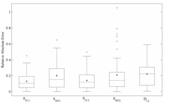
The mean value of RAE on the 45 situations ranged between 0.13 and 0.21 depending on the
estimated parameter (Fig. 2). Estimation of field capacity of both layers (θFC1 and θFC2)
showed relatively lower RAE (mean RAE < 0.15) as compared to the other parameters (0.19
for θWP1 and DL2,0.21 for θWP2). The standard deviation of RAE varied between 0.1 and 0.24.
θFC1 and θFC2 exhibited relatively lower error variability than the other parameters. However,
the quality of estimation of all the parameters varied significantly depending on the situations
and RAE inferior to 10% can be obtained for all parameters.
< Figure 2 here please >
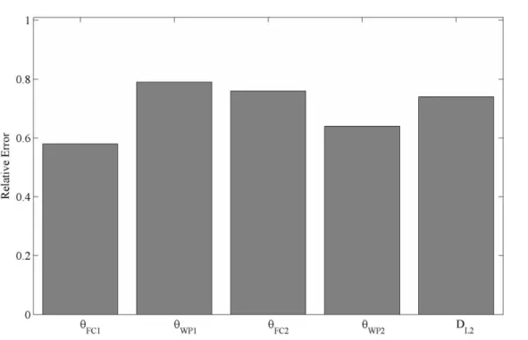
The RE in the estimations was less than 1.0 for all parameters (Fig. 3), indicating that the
inversion improved the accuracy of all the estimated parameters with respect to the mean of
the joint prior distribution. The RE in the estimation was the lowest for θFC1 (0.58) and similar
for θWP1, θFC2 and DL2 (mean value approximately 0.76). For all the parameters RE was less
than 0.80, which is a substantial improvement in the estimation of the parameters with respect
to their prior information.
< Figure 3 here please >
Normalized standard deviation ( ) was largely inferior to 1 for θFC1 and θWC1 (Fig. 4),
18
to the uncertainty associated with the prior information. The reduction of uncertainty for the
second layer parameters (θFC2, θWP2 and DL2) was not so significant. The relatively larger
variability of in the case of θWP1, θFC2 and θWP2 shows that under certain conditions the
uncertainty in the estimates reduced significantly while in some cases the reduction in
uncertainty is only marginal or nil. The level of uncertainty in DL2 is globally closer to that of
prior information even if it can reach 70 to 80% of prior information uncertainty in some
cases.
< Figure 4 here please >
3.2 Effect of crop type
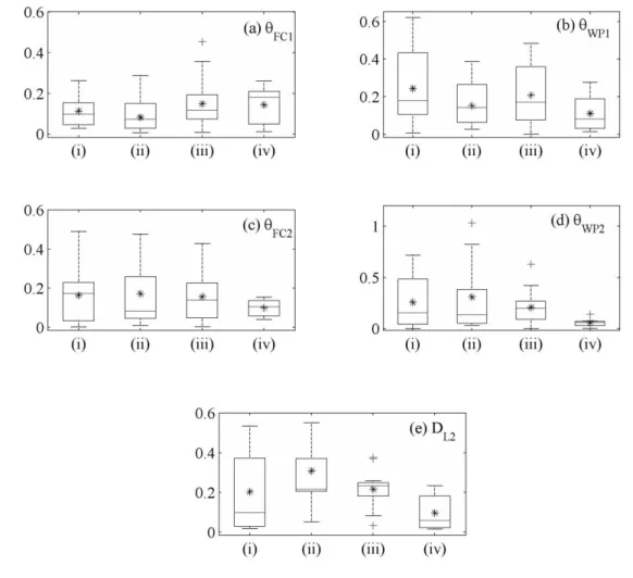
The crop type used for inversion plays an important role in the quality of estimation of the
parameters. This is evident from the consistently lower MRAE of the parameters, except for θFC1, obtained with maize crop as compared to those obtained with the other crops (Fig. 5).
< Figure 5 here please >
The MRAE in the estimation of all parameters except θFC1 were nearly half for maize than
that of the other crops, reaching values of about 10%. One of the main differences between
maize and the other crops concerning the link between root zone hydraulic properties and
crop growth is the water regime experienced by these crops. Due to both climatic conditions
(sunflower and sorghum are grown in rainy season) and management options (irrigation is
mainly devoted to turmeric as it is a cash crop), maize faces drier conditions than the other
crops. Average (Rain+irrigation)/PET ratio was 0.87 for maize against 1.32 for sunflower and
sorghum, and 1.3 for turmeric. STICS model simulations (Fig. 6) confirmed that maize
experienced the maximum stress (both in intensity and duration) as compared to other crops.
19
stress index values is relatively higher, indicating that they experienced different levels of
stress depending on year, soil type or farming practices.
< Figure 6 here please >
The quality of estimation of θFC1 was on the contrary better with sunflower and sorghum as
compared to turmeric and maize. Higher rainfall (and hence higher frequency of high
moisture content conditions in the first layer) occurred during the cropping season of
sunflower and sorghum which would have favored the estimation of θFC1 since SSM
observations can be seen as a proxy of θFC1 in these conditions. For maize, soil moisture data
used for inversion have not attained the actual values of field capacity for all situations
(results not shown).
3.3 Effect of water regime
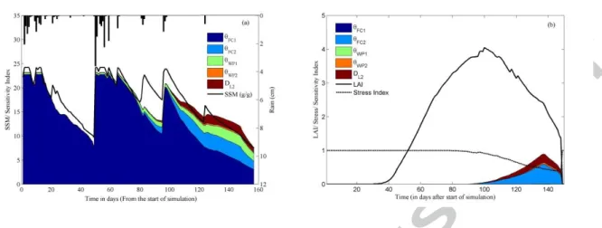
Figure 7 shows dynamics of sensitivity indices of LAI and SSM simulated by the STICS
model to the estimated parameters for a maize plot, representative of the maize plots used in
this study. The variance of SSM explained by the variations of θFC1 clearly follows the
dynamic of simulated SSM: the wetter is the first layer the more the simulated soil moisture is
sensitive to θFC1. This confirms that SSM observed during wet situations contains more
information to estimate this parameter.
< Figure 7 here please >
The influence of the other parameters (θWP1 and second layer parameters) on simulated SSM
starts with the first period of dryness faced by the crop (days 80-95) which coincide with the
beginning of a long water stress period (Fig. 7a). It increases significantly during the
20
continuous increase of water stress. In dry conditions the level of θWP1 limits plant water
uptake in layer one and thus directly affect its moisture content. Second layer parameters also
affect SSM by limiting available water capacity and plant water uptake in second layer and
thus by modifying the repartition of plant water uptake between both layers.
The dynamics of sensitivity indices of LAI to the estimated parameters follow that of the
simulated water stress. In this case, LAI is only sensitive to parameters relative to the second
layer indicating that AWC2 (available water capacity of layer-2, which represent the major
part of total AWC) plays a major role in the dynamic of LAI when the crop is affected by
water stress, as it occurs in this case after the maximum LAI (days 100-150, Fig.7b). Before
this period, the water stress is nil and the sensitivity of LAI to the estimated parameters is
very low.
These results show that the levels of information content in LAI and SSM observations to
estimate AWC components are strongly linked with the water regime and its interaction with
the crop growth. This has been observed for all the situations although the dynamics and
levels of sensitivity indices vary depending on the situations and crops (not shown here).
Impact of the water regime and its interaction with crop growth on the quality of AWC
components estimation is illustrated and quantified in the following subsections.
3.3.3 Surface Layer Properties
As a consequence of the linked patterns of sensitivity of simulated SSM to first layer
parameters and SSM value, the quality of estimation of θFC1 and θWP1 showed a high
dependence on the status of water content in the first layer (Fig. 8).
21
Inversions performed on dry situations (where SSM values were always far from θFC1) yielded
poor estimates of θFC1. On the contrary, situations where at least 3 SSM observations were
available when the first layer was wet (SSM values close to θFC1) provided particularly good
estimates of θFC1 with an error of about 5 % in mean and inferior to 10 % in most cases.
As expected, the opposite behavior was observed for θWP1 since the sensitivity of simulated
SSM to θWP1 was found to be negatively correlated to SSM values (Fig. 7b). Situations in
which at least one observation of SSM was available during period of dryness provided better
estimates of θWP1 than the other situations (Fig. 8b) with errors reduced by approximately
half.
3.3.4 Second layer Properties
Figure 9 shows that the quality of estimation of the second layer properties was related to the
water stress experienced by the crop. Better results were obtained on situations experiencing
large water stress compared to those obtained on situations with no or limited water stress.
The level of water stress experienced by the crop was quantified by S, the proportion of days
in the crop cycle when the water stress index was less than 0.6 (1 corresponds to no stress and
values tending to 0 to very high stress). The error, expressed as MRAE, was relatively lower
in situations where S > 20 % as compared to situations where S < 20 %. In situations where S
> 20 % there was a substantial improvement in the quality of estimation of θFC2 and θWP2,
while DL2 showed only a marginal improvement. The MRAE in the estimation of θWP2 was
reduced by more than half in case of S > 20% as compared to situations where S = 0, reaching
a value inferior to 15%. MRAE of θFC2 was about 10% for S > 20%. Similar results were
22
< Figure 9 here please >
Figure 10 shows that the RAE of the estimation of second layer properties was clearly
negatively correlated with the number of observations of LAI available when the simulated
water stress index was under 0.60. Situations in which at least one LAI observation was
available during period of crop stress considerably improved the estimation of θWP2. For θFC2
at least 2 observations of LAI during period of crop stress were necessary to obtain results
significantly better than when using observations done during periods without stress. We still
notice that the estimation of DL2, even though it is slightly better when LAI observation are
made during stressed periods, still remains poorer than that of θFC2 and θWP2.
< Figure 10 here please >
4.0 Discussion
4.1 Accuracy of estimated soil properties
We have shown that in favorable conditions crop model inversion using observations
potentially available from remote sensing may lead to reasonably accurate estimations of
AWC components of two-layered soils and this even using limited number of observations.
Most of the studies dedicated to the estimation of soil hydraulic properties or AWC
components from model inversion using observations potentially available from remote
sensing are based on synthetic dataset (Jhorar et al., 2002, 2004; Montzka et al., 2011;
Bandara et al., 2013) or on very limited number of real cases (Charoenhirunyingyos et al.,
2011; Sreelash et al., 2012; Shin et al., 2012; Bandara et al., 2014, 2015). However, assessing
23
represents a contribution toward this assessment and confirms the potential utility of this
method.
Further improvements of the estimation errors are still attainable by increasing the level of
information used for the inversion. In addition to observations of model outputs, prior
information on estimated parameters may be used in the inversion process to better constrain
the estimations. A few recent studies (Scharnagl et al., 2011; Scholer et al., 2011), mainly
using hydrological models, have proposed to use soil maps or local texture measurements
combined with hydraulic properties databases or pedotransfer functions to constrain the
inversion problem by using informative prior distributions in Bayesian inversion systems.
This may be particularly helpful for reducing equifinality problems. Thanks to the, sometimes
independent, role played by AWC components in the model, the decoupling in space and time
of the hydric processes affecting the two layers, and the availability of both SSM and LAI
observations in humid and dry conditions, the potential compensation effects between AWC
components were limited. However, compensative effects may still occur in some situations
and this additional information could also help in estimating additional parameters such as
bulk density. The evaluation of the potential of such approaches on large real dataset and
using commonly available data as source of constraints constitutes one of the next key
methodological challenges for the estimation of AWC components from crop model
inversion.
4.2 Effect of hydric regime and its interaction with crop type
We found that the quality of estimation of AWC components was largely dependent on the
hydric regime and its interaction with crop type: field capacity of surface layer was better
estimated in wet conditions whereas wilting point of surface layer and deeper layer properties
24
large set of real data what was partially suggested in (Jhorar et al., 2002; Varella et al., 2010b;
Bandara et al., 2013) mostly on synthetic datasets. Our sensitivity analysis experiments
suggested that this was due to the variation of the level of information content in LAI and
SSM observations. If water inputs from rain or irrigation are not sufficient for ensuring
optimal crop growth then crop growth is highly dependent to AWC and vegetation
measurements bring significant information, particularly on the layers mostly representative
of the root zone. On the contrary if SSM can be seen as a proxy of surface field capacity in
wet conditions, its information content to estimate this property decreases in dry conditions.
This sensitivity analysis also shed light on the results obtained by (Sreelash et al., 2012) about
the complementarity of SSM and LAI observations. In a more general way, these results
confirm the interest of using multiple remotely-sensed constraints for the estimation of
root-zone soil moisture and associated soil properties in model-data fusion systems and the
dependency of their information content on the vegetation state and soil moisture conditions
(Barrett and Renzullo, 2009; Van Dijk and Renzullo, 2011).
Situations which experience large water stress and include wetting and drying cycles are thus
optimal observational objects for estimating AWC components of multi-layered soils from
crop model inversion. The complementary use of a few SSM observations in wet conditions
and LAI observations during water stress period bring significant level of information for
their estimation.
4.3 Impact of errors on the results
The results of the inversions presented in this study are also impacted by different types of
25
(i) model errors (including both errors in the values set for model’s input parameters that are not estimated in the inversions and errors in model’s equations);
(ii) observation errors, i.e. errors on measured LAI and SSM used in the
inversions; and
(iii) reference values errors, i.e. errors on the ‘observed’ values of the AWC
components that are compared to the estimated parameters for assessing their
quality.
Model errors may be linked with model complexity. Complex crop models have been built to
mimic as realistically as possible the different processes involved in crop growth and its
interaction with its environment but the resulting high number of parameters increases the
degrees of freedom in model calibration process and the amount of information needed to
feed the model. This may contribute to decrease model’s robustness (Confalonieri et al.,
2012). The crop model used in this study is representative of the most complex category of
crop models (Jones et al., 2016) and the way parameters and input variables non estimated in
the inversion process are set is conform to the usual practices. Obviously, the limits of the
plant parameters calibration process and the errors on the information used to set its other
entries impact the model simulations as well as do the errors in its equations. The inversions
are based on the computation of the differences between simulated and observed values of
SSM and LAI (SAESSM and SAELAI, eq. 2). This computation is affected in the same way by
model and observation errors and these errors may be compensated by unrealistic values of
the inversed parameters. Errors on SAESSM and SAELAI have been approximated for each
situation by comparing the observed and simulated values of LAI and SSM, using the
reference values of AWC components in simulations. As expected, large SAE errors on LAI
26
variables (results not shown). As practical applications of the method are likely to include
situations with large model and/or observation errors, we didn’t remove such situations from
our analysis, to evaluate as fairly as possible the performance we can expect from this
method. Ensemble modelling has recently shown to be an efficient way of improving crop
simulation (Martre et al., 2015). Although it would be cumbersome to implement, using
several models could be considered in an inversion process to reduce the impact of model
error.
Reference values errors may impact the evaluation of the quality of parameters estimate.
Particularly, the lesser reliability of DL2 measurements in field conditions, as it is difficult to
estimate by augering the precise depth of the base of the soil profile, may partly explain that
its estimation still remains poorer than that of θFC2 and θWP2. In addition, DL2 estimate from
inversion represents an effective soil thickness that might be far from the value assessed in
field conditions. Some particular situations may create such discrepancy between effective
and measured values: presence of an obstacle that prevents the roots to attain the base of the
soil profile and limits the effective AWC, or presence of a transient perched water table
connected with the base of the profile that allows a larger effective AWC than observed.
4.4 Practical application of the method on agricultural catchments
The results presented in this study contribute to evaluate the potential of AWC components
retrieval from crop model inversion and may help to define optimal configuration for the
application of this method on agricultural catchments. This next step is challenging but
necessary to bring solutions to the issue of monitoring water resources in irrigated agricultural
catchments.
Application of this method for deriving soil maps of AWC components would require the use
27
applicable with remote sensed data and the benefit of using them has already been shown in
other studies (Santanello, et al., 2007; Charoenhirunyingyos et al., 2011; Ines et al., 2013;
Bandara et al 2015). In tropical regions, where cloudy conditions are frequent, SSM and LAI
are attainable from radar remote sensing (e.g. Wagner et al., 1999; Tomer et al., 2015 for
SSM ; Kim et al., 2012 ; Hirooka et al., 2015 for LAI).
Crop model inputs such as climate or farming practices are often less precisely known at the
territory scale than at point scale. The level of precision of the available information on these
inputs may impact crop models simulations (Jego et al., 2015). Additional studies would be
required to assess the influence of these uncertainties on the results of the inversions to
evaluate to what extent they impact the quality of AWC components retrieval.
Finally, systematic multi-local application of this method in its current configuration for
deriving soil maps of AWC components in agricultural catchments may face the problem of
vegetation types or crops non-represented in the model and of the dependence of its
performance to the agro-pedo-climatic conditions on which it is applied. It may thus
advantageously be combined with advanced geostatistical methods able to take into account
in an optimal way all kind of existing soil information (McBratney et al., 2003). In this
context, the results presented in this study may guide the sampling of representative fields
over a territory to use this technique for soil mapping exercise.
5.0 Conclusion
In this study we evaluated on an extensive field experiment the potential of crop model
inversion for estimating AWC components on two-layered soils with observations potentially
28
We have shown that:
1) the quality of estimation of AWC components varied depending on the situations on
which it was estimated. These estimations were however systematically better than the
prior information used although this prior information was already of relatively good
quality;
2) the quality of estimation of AWC components was found to largely depend on the
hydric regime and its interaction with crop type: field capacity of surface layer was
better estimated in wet conditions whereas wilting point of surface layer and deeper
layer properties were better estimated in dry conditions and with crops facing hydric
stress;
3) using simultaneously LAI and SSM observations allowed to obtain mean relative
absolute error of 5% for field capacity of surface layer, 10% for field capacity of root
zone, 15% for wilting point of surface layer and root zone, and 20% for soil depth, in
favorable conditions; and
4) a few observations of LAI and SSM available in favorable conditions were sufficient
to largely improve the estimation of AWC components.
We confirmed the utility of the inversion of crop-models to provide realistic soil-water
properties and further improvements such as inclusion of informative prior distributions or
reduction of model error are still conceivable. Further studies are however still needed to
apply this method for deriving soil maps of AWC components at agricultural catchment scale.
Such improvements will allow deriving accurate maps of soil AWC at the catchment scale,
which are essential for distributed hydrological models aimed at studying the impact of
29
Acknowledgements
The funding provided by CNES (Centre National d'Etudes Spatiales) to the first author for
carrying out post-doctoral research is gratefully acknowledged. Apart from the specific
support from the French Institute of Research for Development (IRD), the Embassy of France
in India and the Indian Institute of Science, the research was funded by the Environmental
Research Observatory BVET (http://bvet.obs-mip.fr/en), the Indo-French program IFCPAR
(Indo-French Center for the Promotion of Advanced Research) through the project 4700WA “Adaptation of Irrigated Agriculture to Climate Change” (AICHA) and by the INRA Metaprogramme ACCAF. The authors would like to thank the members of the field team:
Amit Kumar Sharma, Arun Raju, P. Giriraj and K. N. Sanjeeva Murthy and the farmers for
the help provided during the field experiments. Finally, the authors thank the editor, the
associate editor and two anonymous reviewers for their constructive comments which helped
us to substantially improve this manuscript.
References
Anuraga, T.S., Ruiz, L., Kumar, M.S.M., Sekhar, M., Leijnse, A., 2006. Estimating groundwater recharge using land use and soil data: a case study in South India. Agric.
Water Manage. 84, 65–76.
Aronica, G., Bates, P.D. and Horritt, M.S., 2002. Assessing the uncertainty in distributed model predictions using observed binary pattern information within GLUE.
Hydrological Processes. 16(10), 2001-2016. doi: 10.1002/hyp.398
Baghdadi, N., Zribi, M., 2006. Evaluation of radar backscatter models IEM, Oh and Dubois using experimental observations. International Journal of Remote Sensing.
30
Bandara, R., Walker, J.P., Rudiger, C., 2013. Towards soil property retrieval from space: a one dimensional twin experiment. Journal of Hydrology. 497, 198-207. doi:
10.1016/j.jhydrol.2013.06.004
Bandara, R., Walker, J.P., Rudiger, C., 2014. Towards soil property retrieval from space: Proof of concept using in situ observations. Journal of Hydrology. 512, 27-38.
doi: 10.1016/j.jhydrol.2014.02.031
Bandara, R., Walker, J.P., Rudiger, C., Merlin, O., 2015. Towards soil property retrieval from space: An application with disaggregated satellite observations. Journal
of Hydrology. 522, 582-593. doi : 10.1016/j.jhydrol.2015.01.018
Baret, F., 1986. Contribution au suivi radiométrique de cultures de céréales. Phd Thesis Submitted to University of Paris South (Université Paris Sud).
Barrett, D.J., Renzullo, L.J., 2009. On the efficacy of combining thermal and microwave satellite data as observational constraints for root-zone soil moisture
estimation. Journal of Hydrometeorology 10 (5), 1109-1127
Beaujouan, V., Durand, P., Ruiz, L., 2001. Modelling the effect of the spatial distribution of agricultural practises on nitrogen fluxes in rural catchments. Ecological
Modelling. 137(1), 93-105. doi: 10.1016/S0304-3800(00)00435-X
Beven, K.J, Binley, A.M., 1992. The future of distributed models: model calibration and uncertainty prediction. Hydrological Processes. 6(3), 279-298. doi :
10.1002/hyp.3360060305
Botula, Y.D., Cornelis, W.M., Van Ranst, E., 2012. Evaluation of pedotransfer functions for predicting water retention of soils in Lower Congo (D.R. Congo).
31
Braga, R.P., Jones, J.W., 2004. Using optimization to estimate soil inputs of crop models for use in site-specific management. TransActions of the ASAE. 47(5),
1821-1831. doi : 10.13031/2013.17599
Braun, J.J., Descloitres, M., Riotte, J., Fleury, S., Barbiero, L., Boeglin, J.L., Violette, A., Lacarce, E., Ruiz, L., Sekhar, M., Kumar, M.S.M., Subramanian, S., Dupre, B.,
2009. Regolith mass balance inferred from combined mineralogical, geochemical and
geophysical studies: Mule Hole gneissic watershed, South India. Geochimica et
Cosmochimica Acta. 73(4), 935–961. doi: 10.1016/j.gca.2008.11.013
Brazier, R.E., Beven, K.J., Freer, J., Rowan, J.S., 2000. Equifinality and uncertainty in physical based soil erosion models: application of the GLUE methodology to
WEPP-The Water Erosion Prediction Project-for sites in the UK and USA. Earth Surface
Processes and Landforms. 25, 825-845. doi:
10.1002/1096-9837(200008)25:8<825::AID-ESP101>3.0.CO;2-3
Breda, N., Huc, R., Granier, A., Dreyer, E., 2006. Temperate forest trees and stands under severe drought: a review of ecophysiological responses, adaptation processes
and long-term consequences. Annals of Forest Science. 63(6), 625–644. doi:
10.1051/forest:2006042
Brisson, N., Mary, B., Ripoche, D., Jeuffroy, M.H., Ruget, F., Nicoullaud, B., Gate, P., Devienne-Baret, F., Antonioletti, R., Durr, C., Richard, G., Beaudoin, N., Recous,
S., Tayot, X.P.D., Cellier, P., Machet, J.-M., Meynard, J.-M., Delecolle, R., 1998.
STICS: a generic model for simulating crops and their water and nitrogen balances.I.
Theory and parameterization applied to wheat and corn. Agronomie. 18(5-6), 311-346.
32
Brisson, N., Launay, M., Mary, B., Beaudoin, N., 2008. Conceptual basis, formalisations and parameterization of the STICS crop model. QUAE editions,
Versailles Cedex.
Bruand, A., Fernandez, P.N., Duval, O., 2003. Use of class pedotransfer functions based on texture and bulk density of clods to generate water retention curves. Soil Use
and Management. 19(3), 232–242. doi: 10.1111/j.1475-2743.2003.tb00309.x
Buis, S., Wallach, D., Guillaume, S., Varella, H., Lecharpentier, P., Launay, M., Guerif, M., Bergez, J.-E., Justes, E., 2011. The STICS crop model and associated
software for analysis, parameterization, and evaluation. In: L.R. Ahuja, Liwang Ma,
dir., Methods of introducing system models into agricultural research. Advances in
Agricultural Systems Modeling. 2, 395-426.
Charoenhirunyingyos., S, Honda., K., Kamthonkiat., D., Ines., A.V.M., 2011. Soil moisture estimation from inverse modeling using multiple criteria functions. Journal
of Computers and Electronics in Agriculture. 75(2), 278–287. doi:
10.1016/j.compag.2010.12.004
Confalonieri, R., Bregaglio, S., & Acutis, M. (2012). Quantifying plasticity in simulation models. Ecological Modelling, 225, 159-166.
Coucheney, E., Buis, S., Launay, M., Constantin, J., Mary, B., Cortazar-Atauri, I.G., Ripoche, D., Beaudoin, N., Ruget, N., Andrianarisao, K.S., Bas, C.L., Justes, E.,
Leonard, J., 2015. Accuracy, robustness and behaviour of the STICS soil-crop model
for plant, water and nitrogen outputs: Evaluation over a wide range of
argo-environmental conditions in France. Environmental Modelling & Software. 64,
177-190. doi: 10.1016/j.envsoft.2014.11.024
De Vries, J.J., Simmers, I., 2002. Groundwater recharge: an overview of processes and challenges. Hydrogeol. J. 10, 5–17.
33
Guérif, M., Houlès, V., Makowski, D., Lauvernet, C., 2006. Data assimilation and parameter estimation for precision agriculture using the crop model STICS. In:
Wallach, D., Makowski, D., Jones, J.W. (Eds.), Working with Dynamic Crop Models.
Elsevier.
Hirooka, Y., Homma, K., Maki, M., & Sekiguchi, K. (2015). Applicability of synthetic aperture radar (SAR) to evaluate leaf area index (LAI) and its growth rate of rice in farmers’ fields in Lao PDR. Field Crops Research, 176, 119-122.
Hunt, E.D., Hubbard, K.G., Wilhite, D.A., Arkebauer, T.J., Dutcher, A.L., 2009. The development and evaluation of a soil moisture index. International Journal of
Climatology. 29(5), 747-759. doi: 10.1002/joc.1749
Ines, A. V. M., Mohanty, B. P., 2008. Near-surface soil moisture assimilation for quantifying effective soil hydraulic properties under different hydro-climatic
conditions. Vadose Zone Journal. 7, 39–52. doi: 10.2136/vzj2007.0048
Ines, A. V., Das, N. N., Hansen, J. W., & Njoku, E. G. (2013). Assimilation of remotely sensed soil moisture and vegetation with a crop simulation model for maize
yield prediction. Remote Sensing of Environment, 138, 149-164.
Jackson, T.J., Le Vine, D.M., Schmugge, T.J., Schiebe, F.R., 1995. Large area mapping of soil moisture using ESTAR passive microwave radiometer in Washita ’92. Remote Sensing Environment. 53, 27–37. doi: 10.1016/0034-4257(95)00084-E
Jégo G, Pattey E, Mesbah SM, Liu J, Duchesne I. (2015) Impact of the spatial resolution of climatic data and soil physical properties on regional corn yield
predictions using the STICS crop model. International Journal of Applied Earth
34
Jhorar, R.K., Bastiaanssen, W.G.M., Feddes, R.A., Van Dam, J.C., 2002. Inversely estimating soil hydraulic functions using evapotranspiration fluxes. Journal of
Hydrology. 258(1-4), 198-213. doi: 10.1016/S0022-1694(01)00564-9
Jones, J. W., Antle, J. M., Basso, B., Boote, K. J., Conant, R. T., Foster, I., ... & Keating, B. A. (2016). Brief history of agricultural systems modeling. Agricultural
Systems. In press.
Kim, Y., Jackson, T., Bindlish, R., Lee, H., & Hong, S. (2012). Radar vegetation index for estimating the vegetation water content of rice and soybean. IEEE
Geoscience and Remote Sensing Letters, 9(4), 564-568.
Kumar,S., Sekhar, M., Bandyopadhyay, S., 2009. Assimilation of remote sensing and hydrological data using adaptive filtering techniques for watershed modeling. Current
Science. 97(8), 1196–1202.
Lagacherie, P., McBratney, A.B., 2007. Spatial soil information systems and spatial soil inference systems: Perspectives for digital soil mapping. In: Lagacherie, P.;
McBratney, A., Voltz, M., eds. Digital soil mapping: An introductory perspective.
Amsterdam, Elsevier, pp.3-22.
Lagacherie, P., Baret, F., Feret, J.-B., Netto, J.M. and Robbez-Masson, J.M., 2008. Estimation of soil clay and calcium carbonate using laboratory, field and airborne
hyperspectral measurements. Remote Sensing Environment.112, 825-835. doi:
10.1016/j.rse.2007.06.014
Li, C., Ren, Li., 2011. Estimation of unsaturated soil hydraulic parameters using the ensemble kalman filter. Vadose Zone Journal. 10(4), 1205-1227. doi:
10.2136/vzj2010.0159
Li, L., Xia, J., Xu, C.Y., Singh, V.P., 2010. Evaluation of the subjective factors of the GLUE method and comparison with the formal Bayesian method in uncertainty
35
assessment of hydrological models. Journal of Hydrology. 390 (3–4), 210–221. doi:
10.1016/j.jhydrol.2010.06.044
McBartney, A.B., Minasny, B., Cattle, S.R., Vervoort, R.W., 2002. From pedotransfer functions to soil inference systems. Geoderma. 109(1-2), 41-73. doi:
10.1016/S0016-7061(02)00139-8
McBartney, A.B., Santos, M.L.M., Minasny, B., 2003. On digital soil mapping. Geoderma, 117(1-2), 3-52. doi: 10.1016/S0016-7061(03)00223-4
Makowski, D, Wallach, D, Tremblay, M, 2002. Using a Bayesian approach to parameter estimation; comparison of the GLUE and MCMC methods.
Agronomie. 22(2), 191-203. doi: 10.1051/agro:2002007
Makowski, D., Jeuffroy, M. H. Guérif, M., 2004. Bayesian methods for updating crop model predictions, applications for predicting biomass and grain protein content. In :
Bayesian statistics and Quality Modelling in the Agro-Food Production Chain", van
Boekel MAJS, Stein A, Van Bruggen AHC (eds.). Kluwer Academic Publishers,
57-68.
Martinez-Fernandez, J., Gonzalez-Zamora, G., Sanchez, N., Gumuzzio, A,. 2015. A soil water based index as a suitable agricultural drought indicator. Journal of
Hydrology. 522, 265-273. doi: 10.1016/j.jhydrol.2014.12.051
Martre, P., Wallach, D., Asseng, S., Ewert, F., Jones, J. W., Rötter, R. P., ... & Hatfield, J. L. (2015). Multimodel ensembles of wheat growth: many models are better
than one. Global change biology, 21(2), 911-925.
Mckay, M., Beckman, R., Conover, W., 1979. A comparison of three methods for selecting values of input variables in the analysis of output from a computer code.