HAL Id: inria-00589687
https://hal.inria.fr/inria-00589687
Submitted on 30 Apr 2011
HAL is a multi-disciplinary open access
archive for the deposit and dissemination of
sci-entific research documents, whether they are
pub-lished or not. The documents may come from
teaching and research institutions in France or
abroad, or from public or private research centers.
L’archive ouverte pluridisciplinaire HAL, est
destinée au dépôt et à la diffusion de documents
scientifiques de niveau recherche, publiés ou non,
émanant des établissements d’enseignement et de
recherche français ou étrangers, des laboratoires
publics ou privés.
Optimal Time Data Gathering in Wireless Networks
with Omni-Directional Antennas
Jean-Claude Bermond, Luisa Gargano, Stéphane Pérennes, Adele Rescigno,
Ugo Vaccaro
To cite this version:
Jean-Claude Bermond, Luisa Gargano, Stéphane Pérennes, Adele Rescigno, Ugo Vaccaro. Optimal
Time Data Gathering in Wireless Networks with Omni-Directional Antennas. SIROCCO2011, Gdansk
University of technology, Jun 2011, Gdansk, Poland. pp.306-317. �inria-00589687�
Optimal Time Data Gathering in Wireless
Networks with Omni–Directional Antennas
Jean–Claude Bermond1!, Luisa Gargano2, Stephane Per´ennes1,
Adele A. Rescigno2, and Ugo Vaccaro2
1 MASCOTTE, joint project CNRS-INRIA-UNSA, F-06902 Sophia-Antipolis, France 2 Dipartimento di Informatica, Universit`a di Salerno, 84084 Fisciano (SA), Italy
Abstract. We study algorithmic and complexity issues originating from the problem of data gathering in wireless networks. We give an algorithm to construct minimum makespan transmission schedules for data gather-ing when the communication graph G is a tree network, the interference range is any integer m ≥ 2, and no buffering is allowed at intermediate nodes. In the interesting case in which all nodes in the network have to deliver an arbitrary non-zero number of packets, we provide a closed for-mula for the makespan of the optimal gathering schedule. Additionally, we consider the problem of determining the computational complexity of data gathering in general graphs and show that the problem is NP– complete. On the positive side, we design a simple (1 + 2/m) factor approximation algorithm for general networks.
1
Introduction
Technological advances in very large scale integration, wireless networking, and in the manufacturing of low cost, low power digital signal processors, combined with the practical need for real time data collection have resulted in an impressive growth of research activities in Wireless Sensor Networks (WSN). Usually, a WSN consists of a large number of small-sized and low-powered sensors deployed over a geographical area, and of a base station where data sensed by the sensors are collected and accessed by the end user. Typically, all nodes in a WSN are equipped with sensing and data processing capabilities; the nodes communicate with each other by means of a wireless multi-hop networks.
A basic task in a WSN is the systematic gathering at the base station of the sensed data, generally for successive further processing. Due to the current technological limits of WSN, this task must be performed under quite strict constraints. Sensor nodes have low-power radio transceivers and operate with non– replenishable batteries. Data transmitted by a sensor reach only the nodes within the transmission range of the sender. Nodes far from the base station must use intermediate nodes to relay data transmissions. Data collisions, that happen when two or more sensors send data to a common neighbor at the same time, may disrupt the data aggregation process at the base station. An other important factor to take into account when performing data gathering is the
latency of the information accumulation process. Indeed, the data collected by a node of the network can frequently change, thus it is essential that they are received by the base station as soon as it is possible without being delayed by collisions [18]. The same problem was asked by France Telecom (see [6]) on how to bring internet to places where there is no high speed wired access. Typically, several houses in a village want to access a gateway connected to internet (for example via a satellite antenna). To send or receive data from this gateway, they necessarily need a multiple hop relay routing.
All these issues raise unique challenging problems towards the design of effi-cient algorithms for data gathering in wireless networks. It is the purpose of this paper to address some of them and propose effective methods for their solutions. 1.1 The Model
We adopt the network model considered in [1, 2, 9, 10, 14]. The network is rep-resented by a node–weighted graph G = (V, E), where V is the set of nodes and E is the set of edges. More specifically, each node in V represents a device that can transmit and receive data. There is a special node s ∈ V called the Base Station (BS), which is the final destination of all data possessed by the various nodes of the network. Each v ∈ V − {s} has an integer weight w(v) ≥ 0, that represents the number of data packets it has to transmit to s. Each node is equipped with an half–duplex transmission interface, that is, the node cannot transmit and receive at the same time. There is an edge between two nodes u and v if they can communicate. So G = (V, E) represents the graph of possible communications. Some authors consider that two nodes can communicate only if their distance in the Euclidean space is less than some value. Here we con-sider general graphs in order to take into account physical or social constraints, like walls, hills, impediments, etc.. In that context paths and trees represent the cases where the communications are done with antennas only in few directions or urban situations with possible communications only along streets. Furthermore, many transmission protocols use a tree of shortest paths for routing.
Time is slotted so that one–hop transmission of a packet (one data item) con-sumes one time slot; the network is assumed to be synchronous. These hypotheses are strong ones and suppose a centralized view. The values of the completion time we obtain will give lower bounds for the corresponding real life values. Said otherwise, if we fix a value on the completion time, our results will give an upper bound on the number of possible users in the network.
Following [10, 12, 18], we assume that no buffering is done at intermediate nodes and each node forwards a packet as soon as it receives it. One of the rationales behind this assumption is that it might be too much energy consuming to hold data in the node memory; moreover, it also free intermediate nodes from the need to maintain costly state information.
Finally we use a binary model of interference based on the distance in the communication graph. Let d(u, v) denote the distance (that is, the length of a shortest path) between u and v in G. We suppose that when a node u trans-mits, all nodes v such that d(u, v) ≤ m are subject to the interference of u’s
transmission and cannot receive any packet from their neighbors. This model is a simplified version of the reality, where a node is under the interference of all the other nodes and where models based on SNR (Signal-to-Noise Ratio) are used. However our model is more accurate compared to the classical binary model (m = 1), where a node cannot receive a packet only in the case one of its neighbor transmits. We suppose all nodes have the same interference range m; in fact m is only an upper bound on the possible range of interferences since due to obstacles the range can be sometimes lower (however, see also [17] for a critique of this model).
Under above model, simultaneous transmissions among pair of nodes are suc-cessful whenever transmission and interference constraints are respected. Namely, a transmission from node v to w is called collision–free if, for all simultaneous transmissions from any node x, it holds: d(v, w) = 1 and d(x, w) ≥ m + 1. The gathering process is called collision–free if each scheduled transmission is collision–free. The collision–free data gathering problem can be stated as follows. Data Gathering. Given a graph G = (V, E), a weight function w : V → N , and a base station s, for each node v ∈ V −{s} schedule the multi-hop transmission of the w(v) data items sensed at node v to base station s so that the whole process is collision–free and the makespan, i.e., the time when the last data item is received by s, is minimized.
Actually, we will describe the gathering schedule by illustrating the schedule for the equivalent personalized broadcast problem, since this last formulation allows us to use a simpler notation.
Personalized broadcast: Given a graph G, a weight function w : V → N , and a BS s, for each node v &= s schedule the multi-hop transmission from s to v of the w(v) data items destined to v so that the whole process is collision– free and the makespan, i.e., the time when the last data item is received at the corresponding destination node, is minimized.
We notice that any collision–free schedule for the personalized broadcasting prob-lem is equivalent to a collision–free schedule for data gathering. Indeed, let T be the last time slot used by a collision–free personalized broadcasting schedule; any transmission from a node v to its neighbor w occurring at time slot k in the broadcasting schedule corresponds to a transmission from w to v scheduled at time slot T + 1 − k in the gathering schedule. Moreover, if two transmissions in the broadcasting schedule, say from node v to w and from v!to w!, do not collide
then d(v!, w), d(v, w!) ≥ m + 1; this implies that, in the gathering schedule, the
corresponding transmissions from w to v and from w! to w do not collide either.
Hence, if one has an (optimal) broadcasting schedule from s, then one can get an (optimal) solution for gathering at s.
Let S be a personalized broadcasting schedule for the graph G and BS s. We denote by TS the makespan of S, i.e., the last time slot in which a packet is
sent along any edge of the graph. Moreover, we denote by TS(x) the time slot
the execution of the schedule S. Clearly, the makespan of S is
TS = max {dS(s, x) + TS(x) | x ∈ V, w(x) > 0} , (1)
where dS(s, x) is the number of hops used in S for a packet to reach x.
The makespan of an optimal schedule3 is T∗(G, s) = minSTS, where the
minimum is taken over all collision-free personalized broadcasting schedules for the graph G and BS s. When s is clear from the context, we simply write T∗(G)
to denote the optimal makespan value. 1.2 Our Results and Related Work
Our first result is presented in Section 2, where we give an algorithm to determine an optimal transmission schedule for data gathering (personalized broadcasting) in case the communication graph G is a tree network and the interference range is any integer m ≥ 2. Our algorithm works for general weight functions w on the set of nodes V of G. In the interesting case in which the weight function w assume non-zero values on V we are also able to determine a closed formula for the makespan of the optimal gathering schedule. The papers most closely related to our results are [2, 10, 12]. Paper [10] firstly introduced the data gathering problem in a model for sensor networks very similar to the one adopted in this paper. The main difference with our work is that [10] mainly deals with the case where nodes are equipped with directional antennas, that is, only the designated neighbor of a transmitting node receives the signal while its other neighbors can simultaneously and safely receive from different nodes. Under this assumption, [10] gives optimal gathering schedules for trees. Again under the same hypothesis, an optimal algorithm for general networks has been presented in [12] in the case each node has one packet of sensed data to deliver. Paper [2] gives optimal gathering algorithms for tree networks in the same model considered in the present paper, but the authors consider only the particular case of interference range m = 1. It is worthwhile to notice that, although our results hold for general interference range m ≥ 2, our algorithms (and analysis thereof) are much cleaner and simpler than those for m = 1. In view of our results, it really appears that the case of interference range m = 1 has a peculiar behavior, justifying the quite detailed case analysis of [2].
Other related results appear in [1, 4, 5, 7], where fast gathering with omni-directional antennas is considered under the assumption of possibly different transmission and interference ranges. That is, when a node transmits all the nodes within a fixed distance dT in the graph can receive, while nodes within
distance dI (dI ≥ dT) cannot listen to other transmissions due to interference
(in our paper dI = m and dT = 1). However, unlike the present paper, all of the
above works explicitly allow data buffering at intermediate nodes.
In Section 4, we consider the problem of assessing the hardness of data gathering
3 Note that, by the equivalence between data gathering and personalized broadcasting,
in the following we will use T∗(G) to denote interchangeably the makespan of the
in general graphs and show that the problem is NP–complete. In Section 3 we give a simple (1 + 2/m) factor approximation algorithm for general networks.
Due to space limits, most of the proofs are omitted. The full version of the paper is available on ArXiv.
2
Scheduling in Trees
In this section we describe scheduling algorithms when the network topology is a tree T = (V, E). We first give a polynomial time algorithm for obtaining optimal personalized broadcast schedules in case of strictly positive node weights. Subsequently, in the general case when some nodes can have zero weight, we derive an O(δW3δ) algorithm for obtaining an optimal schedule, where W is
the sum of the weights of the nodes in the network (number of data packets transmitted) and δ is the BS degree.
Let T1, T2, · · · , Tδ be the subtrees of T rooted at the children of the BS s.
In order to describe the scheduling, we use the following nomenclature. – At time t: During the t-th time slot (one time slot corresponding to a one
hop transmission of one packet).
– Transmit to node v at time t: a packet to v is sent along a path (s = x0, x1, · · · , x#= v) from s to v in T starting at time t, that is, the packet is
transmitted with a call from xj to xj+1 at step t + j, for j = 0, · · · , " − 1.
– Node v is completed (at time t): s has already transmitted all the w(v) packets to v (within some time t!< t).
– Transmit to Ti at time t: a packet is transmitted at time t to a node v in Ti,
where v is chosen as the node having maximum level among all nodes in Ti
which are not completed at time t.
– Ti is completed: each node v in Ti is completed.
Fact 1 Let s transmit to a node u ∈ V (Ti) at time t and to node v ∈ V (Tj) at
time t! > t. The calls done during the transmission from s to u and the calls
of the transmission from s to v do not interfere if and only if t! ≥ t + ∆(u, v),
where the inter–call interval ∆(u, v) is defined as ∆(u, v) =
!
min{d(s, u), m} if i &= j,
min{d(s, u), m + 2} if i = j. (2)
2.1 Trees with non–zero node weights
In this section we show how to obtain an optimal transmission schedule of the packets to the nodes in a tree T when w(v) ≥ 1, for each node v in T .
For each subtree Ti of T , for i = 1, . . . , δ, we denote by
– si the root of Ti;
– |Ai| ="v∈Aiw(v): the total weight of the nodes in Ai= {v ∈ V (Ti) | d(s, v) ≤
m}, that is, of the nodes in Ti that are at level at most m in T ;
– |Bi| ="v∈Biw(v): the total weight of all the nodes in Bi= {v ∈ V (Ti) | d(s, v) =
– |Ci| ="v∈Ciw(v): the total weight of all the nodes in Ci= {v ∈ V (Ti) | d(s, v) ≥
m + 2}, that is, of the nodes in Ti that are at level m + 2 or more in T ;
– |Ti|: the total weight of nodes in Ti, that is, |Ti| = |Ai| + |Bi| + |Ci|.
Definition 1 Given i, j = 1, . . . , δ with i &= j, we say that
Ti' Tj if |Bi| + |Ci| ≥ |Bj| + |Cj| whenever |Bi| + |Ci| > 0, |Ai| − w(si) ≥ |Aj| − w(sj) whenever |Bi| + |Ci| = |Bj| + |Cj| = 0, |Ai| > w(si) w(si) ≥ w(sj) whenever |Ti| = w(si) and |Tj| = w(sj)
Theorem 1 Let the interference range be m ≥ 2. Let T be a tree with node weight w(v) ≥ 1, for each v ∈ V . Consider T as rooted at the BS s and (w.l.o.g.) let its subtrees be indexed so that T1' T2' . . . ' Tδ. There exists a polynomial
time scheduling algorithm S for T such that TS = T∗(T ) = ' u∈V d(s,u)≤m w(u)d(s, u) + m δ ' i=1 (|Bi| + |Ci|) + M, (3) where M = max{0, (|B1| + |C1|) − δ ' i=2 |Ti|, (|B1| + 2|C1|) + δ ' i=2 w(si) − 2 δ ' i=2 |Ti|} (4)
Proof (Sketch). The proof consists in showing that the value in the statement of Theorem 1 is a lower bound on the makespan of any schedule. Subsequently, we prove that the scheduling algorithm given in Figure 1 is collision-free and its
makespan matches the lower bound. ()
We notice that in the special case δ = 1, Theorem 1 reduces to
Corollary 1 [10] Let L be a line with nodes {0, 1, . . . , n}, BS at node 0, and let w(") ≥ 1 be the weight of node ", for " = 1, . . . , n. Then T∗(L) ="m+1
#=1 " ·
w(") + (m + 2)"
#≥m+2w(").
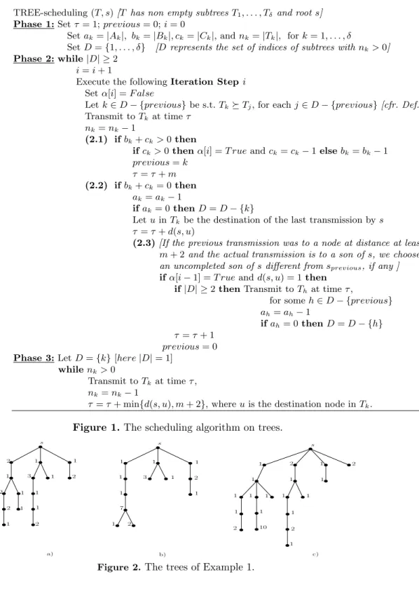
Example 1. We stress that each of the values of M in (4) is attained by some tree. Figure 2 shows an example for each case assuming the interference range be m = 3. The vertices of the trees are labeled with their weights and the subtrees are ordered from left to right according to Definition 1.
a) Consider the tree T in Fig.2 a). T has subtrees T1, T2, T3 with |B1| = 3,
|C1| = 1, |T2| + |T3| = 12 and w(s2) + w(s3) = 2. Therefore, |B1| + |C1| − (|T2| +
|T3|) = −8 < 0 and |B1| + 2|C1| + (w(s2) + w(s3)) − 2(|T2| + |T3|) = −17 < 0.
Hence, M = 0 in this case.
b) Consider the tree T in Fig.2 b). T has subtrees T1, T2, T3 with |B1| = 7,
|C1| = 3, |T2| + |T3| = 9 and w(s2) + w(s3) = 2. Therefore, |B1| + |C1| − (|T2| +
|T3|) = 1 > 0 and |B1| + 2|C1| + (w(s2) + w(s3)) − 2(|T2| + |T3|) = −3 < 0.
Hence, M = |B1| + |C1| −"δi=2|Ti| in this case.
c) Consider the tree T in Fig.2 c). T has subtrees T1, T2, T3, T4 with |B1| = 2,
|C1| = 12, |T2| + |T3| + |T4| = 13 and w(s2) + w(s3) + w(s4) = 5. Therefore,
|B1|+|C1|−(|T2|+|T3|+|T4|) = 1 > 0 and |B1|+2|C1|+(w(s2)+w(s3)+w(s4))−
TREE-scheduling (T, s) [T has non empty subtrees T1, . . . , Tδ and root s]
Phase 1: Set τ = 1; previous = 0; i = 0
Set ak= |Ak|, bk= |Bk|, ck= |Ck|, and nk= |Tk|, for k = 1, . . . , δ
Set D = {1, . . . , δ} [D represents the set of indices of subtrees with nk> 0]
Phase 2: while |D| ≥ 2 i = i + 1
Execute the following Iteration Step i Set α[i] = F alse
Let k ∈ D − {previous} be s.t. Tk$ Tj, for each j ∈ D − {previous} [cfr. Def. 1]
Transmit to Tkat time τ
nk= nk− 1
(2.1) if bk+ ck> 0 then
if ck> 0 then α[i] = T rue and ck= ck− 1 else bk= bk− 1
previous = k τ = τ + m (2.2) if bk+ ck= 0 then
ak= ak− 1
if ak= 0 then D = D − {k}
Let u in Tkbe the destination of the last transmission by s
τ = τ + d(s, u)
(2.3) [If the previous transmission was to a node at distance at least m + 2 and the actual transmission is to a son of s, we choose an uncompleted son of s different from sprevious, if any ]
if α[i − 1] = T rue and d(s, u) = 1 then if |D| ≥ 2 then Transmit to That time τ ,
for some h ∈ D − {previous} ah= ah− 1
if ah= 0 then D = D − {h}
τ = τ + 1 previous = 0 Phase 3: Let D = {k} [here |D| = 1]
while nk> 0
Transmit to Tkat time τ ,
nk= nk− 1
τ = τ + min{d(s, u), m + 2}, where u is the destination node in Tk.
Figure 1. The scheduling algorithm on trees.
s 1 1 1 1 3 1 1 1 7 1 2 2 a) b) c) 2 s 2 1 1 1 3 1 2 1 1 2 1 1 2 1 s 1 1 2 1 1 1 1 1 1 1 10 2 1 1 1 2 1 1 2
2.2 Trees with general weight distribution
In this section we present an algorithm for the general case in which only some of the nodes needs to receive packets from the BS s.
Let T = (V, E) be the tree representing the network, and let s be the root of T . Denote by δ the degree of s, and by T1, T2, · · · , Tδ the subtrees of T rooted
at the children of s. We present an algorithm which gives an optimal schedule in time O(δW3δ), where W is the number of items to be transmitted (i.e, the
sum of the weights). However, for sake of simplicity, in the following we limit our analysis to the case w(v) ∈ {0, 1}, for each v ∈ V − {s}.
Lemma 1 For each u, v ∈ V , if either of the following conditions hold a) 2 ≤ d(s, u) < d(s, v) ≤ m
b) d(s, u) > d(s, v) ≥ m + 2 and u, v ∈ V (Ti), for some 1 ≤ i ≤ δ,
then there exists an optimal schedule where s transmits to u before than to v. Based on Lemma 1, we consider the lists Ci, Bi, Ai, for i = 1, . . . , δ, where:
Ci= (xi,1, xi,2, · · · ) consists of all the nodes in Tiwith w(xi,j) > 0 and d(s, xi,j) ≥
m + 2; nodes are ordered so that d(s, xi,j) ≤ d(s, xi,j+1) for each j ≥ 1;
Bi = (zi,1, zi,2, · · · ) consists of all the nodes in Tiwith w(zi,j) > 0 and d(s, zi,j) =
m + 1; in any order;
Ai = (yi,1, yi,2, · · · ) consists of all the nodes in Ti with w(yi,j) > 0 and 2 ≤
d(s, yi,j) ≤ m; nodes are ordered so that d(s, yi,j) ≥ d(s, yi,j+1) for j ≥ 1.
Given integers ci≤ |Ci|, bi ≤ |Bi|, ai ≤ |Ai|, ri ∈ {0, 1}, for i = 1, . . . δ, let
S(c1, . . . , cδ, b1, . . . , bδ, a1, . . . , aδ, r1, . . . , rδ), denote an optimal schedule
satisfy-ing Lemma 1 when the only packets to be transmitted are destined to the first ci nodes of Ci, bi nodes of Bi, ai nodes of Ai, respectively, and, if ri = 1,
to the root si of Ti, for i = 1, . . . , δ. In the following we will use the compact
vectorial notation
c = (c1, · · · , cδ), b = (b1, · · · , bδ) a = (a1, · · · , aδ) r = (r1, · · · , rδ).
Therefore, we write S(c, b, a, r) for S(c1, · · · , cδ, b1, · · · , bδ, a1, · · · , aδ, r1, · · · , rδ).
Moreover, let S(c, b, a, r, (j, t)) be an optimal schedule satisfying above condi-tion and the addicondi-tional restriccondi-tion that the first transmission in the schedule is to a node in Tj where t ∈ {r, C, B, A} specifies whether this node is either the
root of Tj, or a node in Cj (by Lemma 1, node xj,cj), or a node in Bj, or in Aj
(by Lemma 1, node yj,aj).
The makespan of the schedule S(c, b, a, r) (resp. S(c, b, a, r, (j, t))) will be denoted by T (c, b, a, r) (resp. T (c, b, a, r, (j, t))). Clearly,
T (c, b, a, r) = min
1≤j≤δ t∈{r,C,B,A}min T (c, b, a, r, (j, t)). (5)
Denote by eithe identity vector ei= (ei,1, · · · , ei,δ) with ei,j=
!
1 if j = i, 0 otherwise. The following result is an immediate consequence of Fact 1.
Fact 2 For any j = 1, · · · , δ, it holds
– if t = r, then T (c, b, a, r, (j, r)) = 1 + T (c, b, a, r − ej)
– if t = A, then T (c, b, a, r, (j, A)) = d(s, yj,aj) + T (c, b, a − ej, r).
– if t = B, i.e., the first transmission is for zj,bj,∈ Bj, then
T (c, b, a, r, (j, B)) = min k, t! m + T (c, b − ej, a, r, (k, t!)) if j &= k and d(s, zj,bj) ≤ T (c, b − ej, a, r, (k, t !)) + m m + 1 + T (c, b − ej, a, r, (k, t!)) if j = k and d(s, zj,bj) ≤ T (c, b − ej, a, r, (k, t !)) + m + 1 d(s, zj,bj) otherwise
– if t = C, i.e., the first transmission is for xj,cj,∈ Cj, then
T (c, b, a, r, (j, C)) = min k, t! m + T (c − ej, b, a, r, (k, t!)) if j &= k and d(s, xj,cj) ≤ T (c − ej, b, a, r, (k, t !)) + m m + 2 + T (c − ej, b, a, r, (k, t!)) if j = k and d(s, xj,cj) ≤ T (c − ej, b, a, r, (k, t !)) + m + 2 d(s, xj,cj) otherwise
An optimal schedule for T is S(T ) = S(cT, bT, aT, rT), where (cT, bT, aT, rT)
includes all the packets in T . In order to obtain the optimal solution we compute the various partial solutions for (c, b, a, r, (j, t)); starting from T (0, 0, 0, 0, (j, t)) = 0, for each j and t, where 0 = (0, . . . , 0) is the null vector.
We know that ck+ bk+ ak ≤ "v∈V w(v) = W and rk ∈ {0, 1}, for k =
1, · · · , δ; moreover, the pair (j, t) can assume at most 4δ values. Therefore, since w(v) ∈ {0, 1} for each v ∈ V , we get W ≤ |V | and the number of different values we need to compute is O(δ|V |3δ).
For general weights, each node v needs to appear in the proper list (among Ai, Bi, and Ci, for i = 1, . . . , δ) with multiplicity equal to w(v). Hence, our result
assumes the following form.
Theorem 2 It is possible to obtain an optimal schedule in time O(δW3δ).
3
General Topologies
We present an algorithm for Personalized Broadcasting in general graphs and prove that it achieves an approximation ratio of 1+m2, where m is the interference range. We then show that if one requires that the personalized broadcasting has to be done using a routing tree, then the problem is NP–complete. We stress that this practical requirement is widely adopted, indeed it avoids that intermediate nodes have to forward data in a way that depends on source and destination information. The same scenario for m = 1 is considered in [9].
3.1 The approximation algorithm
Consider an arbitrary topology graph G = (V, E) with BS s and node weight w(v) ≥ 0, v ∈ V − {s}. Let SP be a set of shortest paths from s to each node in V − {s}. We route transmissions along the paths in SP .
Graph-SPschedule(G, SP, s) Set t = 1; h = maxu∈V d(s, u)
Set w#="v∈V,d(s,v)=#w(v), for " = 1, . . . , h
while "
#w#> 0
Let L = max{"|w#> 0}
Establish an (arbitrary) ordering on the wL packets to be transmitted
to nodes at distance L from s For j = 1 to wL
s transmits at time t the j–th data packet in the above ordering t = t + min{L, m + 2}
wL= 0
Figure 3. The general graphs scheduling algorithm.
Lemma 2 The makespan of the schedule produced by Graph-SPschedule(G, SP, s) is max! " v∈V d(s,v)≤m+1 w(v)d(s, v) + (m + 2) " v∈V d(s,v)≥m+2 w(v), max #≥m+2#$ − m − 2+ (m + 2) " v∈V d(s,v)≥# w(v)$% .
The analysis of the algorithm would be very simple if we had to deal only with trees (indeed schedules with optimal makespan for trees are given in Sections 2). However, even if we restrict ourselves to packets transmission on a (shortest path) tree, we still need to deal with possible collisions due to the edges in E − E(SP ). In order to see that our algorithm does not suffer from interferences, let us first notice that if (u, v) ∈ E then |d(s, u) − d(s, v)| ≤ 1. Moreover, if s transmits to u at time t and to v at time t!> t then the Graph-SPschedule algorithm imposes
that t!= t + min{d(s, u), m + 2}. By this, as in Fact 1, we get that no collision
occurs during the execution of Graph-SPschedule.
Theorem 3 Let G = (V, E) be a graph with BS s ∈ V and w(u) ≥ 0, for each u ∈ V −{s}, and let the interference range be m. The makespan T of the schedule produced by Graph-SPschedule(G, SP, s) satisfies
T
T∗(G) ≤ 1 +
2 m,
4
Complexity Results
We now show that the Data Gathering Problem is NP-complete if the process must be performed along the edges of a routing tree.
Our proof assumes m ≥ 2. The case m = 1 is claimed to be NP-complete in [9]; however the proof is incorrect. Firstly, it uses invalid results concerning trees. Indeed the authors claim that in the case m = 1, a tree with n vertices and weight 1 in each node has makespan equal to 3n − 2. As a counterexample, consider the tree formed by δ paths of length 2 sharing the node s, so with n = 2δ + 1 nodes. The makespan in this case is 2δ = n − 1 (see [2] for exact values for trees). As a matter of fact, the value in [9] is true only for paths with BS at one end. Additionally, one can easily see that the reduction employed in [9] is, in general, not computable in polynomial time.
To prove our NP-completeness result, let us consider the decision version of the equivalent Minimum Time Personalized Broadcasting.
MTPB (Minimum Time Personalized Broadcasting)
Instance: A graph G = (V, E), an interference range m, a special node s ∈ V , integer weights w(v) ≥ 0 for v ∈ V − {s}, and an integer bound K.
Question: Is there a routing tree in G and a multi-hop schedule on it of the w(v) packets from s to node v, for each v ∈ V , so that the process is collision–free and the makespan is T ≤ K?
We show now that MTPB is NP-complete. It is clearly in NP. We prove its NP-hardness by a reduction from the well known Partition Problem [13]. PARTITION
Instance: n + 1 integers a1, a2, · · · , an, B such that"ni=1ai= 2B.
Question: Is there a subset S ⊂ {1, 2, · · · , n} such that"
i∈Sai= B?
Given a PARTITION instance, we construct a MTPB instance as follows: – The graph is G = (V, E) with node set
V =(s} ∪ {u0 j, vj0| 1 ≤ j ≤ m + n + 1) ∪ (uij, vji | 1 ≤ i ≤ n, 0 ≤ j ≤ m ) ∪(xi | 1 ≤ i ≤ n) , edge set E = {(s, u01), (s, v10)} ∪ {(u0j, u 0 j+1), (v0j, v 0 j+1) | 1 ≤ j ≤ m + n} ∪ {(u0m+n+1, u10), (vm+n+10 , v01)} ∪ {(uij, uij+1), (vji, vj+1i ) | 1 ≤ i ≤ n, 0 ≤ j ≤ m − 1}
∪ {(ui1, ui+10 ), (v1i, vi+10 ) | 1 ≤ i ≤ n − 1}
∪ {(ui
m, xi), (vim, xi) | 1 ≤ i ≤ n};
and node weights w(u0 j) = w(v0j) = 0, for j = 1 . . . , m + 1, w(u0 j) = w(v0j) = 1, for j = m + 2 . . . , m + n + 1, w(ui j) = w(vji) = 0, for i = 1 . . . , n and j = 0 . . . , m, w(xi) = a i, for i = 1 . . . , n.
– The interference parameter is a fixed integer m ≥ 2; – The bound is K = 2m(B + n) + 2.
We notice that the graph G can be constructed in polynomial-time. Moreover, it can be shown that the PARTITION instance admits an answer “Yes” if and only if there exists a schedule for the MTPB instance such that the makespan is T ≤ K. Hence we get
Theorem 4 The MTPB problem is NP-complete.
References
1. Bermond J-C., Galtier J., Klasing R., Morales N., P´erennes S.: Hardness and approximation of gathering in static radio networks. PPL 16 (2), 165–183 (2006). 2. Bermond J-C., Gargano L., Rescigno A.: Gathering with Minimum Delay in Sensor
Networks. Proc. SIROCCO 2008, LNCS 5058, 262–276 (2008).
3. Bermond J-C., Correa R., Yu M.-L.: Optimal Gathering Protocols on Paths under Interference Constraints. Discrete Mathematics 309(18), 5574–5587 (2009). 4. Bermond J-C., Peters J.: Efficient gathering in radio grids with interference. Proc.
AlgoTel’05, Presqu’ˆıle de Giens, 103–106 (2005).
5. Bermond J-C., Yu M.-L.: Optimal gathering algorithms in multi-hop radio tree networks with interferences. Ad Hoc and S.W.N., 9 (1–2), 109–128 (2010). 6. Bertin P., Bresse J-F., Le Sage B.: Acc`es haut d´ebit en zone rurale: une solution
“ad hoc”. France Telecom R&D 22, 16–18 (2005).
7. Bonifaci V., Korteweg P., Marchetti-Spaccamela A., Stougie L.: An Approximation Algorithm for the Wireless Gathering Problem. Op. Res. Lett. 36 (5), 605–608 (2008).
8. Bonifaci V., Klasing R., Korteweg P., Marchetti-Spaccamela A., Stougie L.: Data Gathering in Wireless Networks. Graphs and Algorithms in Communication Net-works, A.Koster and X. Munoz editors, Springer Monograph, 357–377 (2010). 9. Choi H., Wang J., Hughes E.A.: Scheduling for information gathering on sensor
network. Wireless Network 15, 127–140 (2009).
10. Florens C., Franceschetti M., McEliece R.J.: Lower Bounds on Data Collection Time in Sensory Networks. IEEE J. on SAC. 22 (6), 1110–1120 (2004).
11. Gargano L.: Time Optimal Gathering in Sensor Networks. Proc. SIROCCO 2007, LNCS 4474, 7-10 (2007).
12. Gargano L., Rescigno A.A.: Optimally Fast Data Gathering in Sensor Networks. Discrete Applied Mathematics 157, 1858–1872 (2009).
13. Garey M. R., Johnson D. S.: Computers and Intractability: A Guide to the Theory of NP-Completeness. W. H. Freeman (1979)
14. Gasieniec L.,Potapov I.: Gossiping with Unit Messages in Known Radio Networks. IFIP TCS, 193–205 (2002).
15. Pelc A.: Broadcasting in radio networks. Handbook of Wireless Networks and Mo-bile Computing, I. Stojmenovic, Ed. John Wiley and Sons, Inc., 509–528 (2002). 16. Revah Y., Segal M.: Improved bounds for data-gathering time in sensor networks.
Computer Communications 31(17), 4026–4034 (2008).
17. Schmid S., Wattenhofer R: Algorithmic models for sensor networks. IPDPS 2006 18. X. Zhu, Tang B., Gupta H.: Delay efficient data gathering in sensor networks, Proc.