HAL Id: hal-01360662
https://hal.archives-ouvertes.fr/hal-01360662
Submitted on 6 Sep 2016
HAL is a multi-disciplinary open access
archive for the deposit and dissemination of
sci-entific research documents, whether they are
pub-lished or not. The documents may come from
teaching and research institutions in France or
abroad, or from public or private research centers.
L’archive ouverte pluridisciplinaire HAL, est
destinée au dépôt et à la diffusion de documents
scientifiques de niveau recherche, publiés ou non,
émanant des établissements d’enseignement et de
recherche français ou étrangers, des laboratoires
publics ou privés.
Capability of GLAS/ICESat data to estimate forest
canopy height and volume in mountainous forests of Iran
M.R. Pourrahmati, N. Baghdadi, A. Asghar Darvishsefat, M. Namiranian, I.
Fayad, Jean-Stéphane Bailly, V. Gond
To cite this version:
M.R. Pourrahmati, N. Baghdadi, A. Asghar Darvishsefat, M. Namiranian, I. Fayad, et al.. Capability
of GLAS/ICESat data to estimate forest canopy height and volume in mountainous forests of Iran.
IEEE Journal of Selected Topics in Applied Earth Observations and Remote Sensing, IEEE, 2015, 8
(11), pp.5246-5261. �10.1109/jstars.2015.2478478�. �hal-01360662�
Abstract—The importance of measuring biophysical properties of forest for ecosystem health monitoring and forest management encourages researchers to find precise, yet low-cost methods especially in mountainous and large area. In the present study Geoscience Laser Altimeter System (GLAS) on board ICESat was used to estimate three biophysical characteristics of forests
located in north of Iran: 1) maximum canopy height (Hmax), 2)
Lorey’s height (HLorey), and 3) Forest volume (V). A large
number of Multiple Linear Regressions (MLR) and also Random Forest (RF) regressions were developed using different set of variables: waveform metrics, Principal Components (PCs) produced from Principal Component Analysis (PCA) and
Wavelet Coefficients (WCs) generated from wavelet
transformation. To validate and compare different models, statistical criteria were calculated based on a five-fold cross validation. Best model concerning the maximum height was an MLR with an RMSE of 5.0m which combined two metrics
extracted from waveforms (waveform extent "Wext" and height
at 50% of waveform energy "H50"), and one from the Digital
Elevation Model (Terrain Index: TI). The mean absolute error (MAPE) of maximum height estimates is about 16.4%. For
Lorey’s height, a simple MLR model including two metrics (Wext
and TI) represents the highest performance (RMSE=5.1m,
MAPE=24.0%). Totally, MLR models showed better
performance rather than RF models, and accuracy of height estimations using waveform metrics was greater than those based on PCs or WCs. Concerning forest volume, employing regression models to estimate volume directly from GLAS data led to a
better result (RMSE=128.8 m3/ha) rather than volume-HLorey
relationship (RMSE=167.8m3/ha).
The paper was submitted on April xx, 2015. This research was supported in part by Iran National Science Foundation (INSF) and Cotutelle (an international joint PhD program initiated by France).
M. R. Pourrahmati is with IRSTEA, UMR TETIS, 34093 Montpellier, France (e-mail: author@ boulder.nist.gov), and Faculty of Natural Resources, University of Tehran, Karaj, Iran (e-mail: mrajabpour@ut.ac.ir).
N. Baghdadi is with IRSTEA, UMR TETIS, 34093 Montpellier, France (e-mail: nicolas.baghdadi@teledetection.fr).
A.A. Darvishsefat is with Faculty of Natural Resources, University of Tehran, Karaj, Iran (e-mail: adarvish@ut.ac.ir).
M. Namiranian is with Faculty of Natural Resources, University of Tehran, Karaj, Iran (e-mail: mnamiri@ut.ac.ir).
I. Fayad is with IRSTEA, UMR TETIS, 34093 Montpellier, France (e-mail: ibrahim.fayad@teledetection.fr).
J.S. Bailly is with AgroParisTech, UMR LISAH, 34093 Montpellier Cedex 5, France (bailly@agroparistech.fr)
V. Gond is with CIRAD, UPR B&SEF, campus international de Baillarguet, Montpellier, France (valery.gond@cirad.fr)
Index Terms—Forest volume, GLAS/ICESat, Iran, Lidar, Lorey’s height, Maximum height.
I. INTRODUCTION
Forest volume, measured in cubic meters per hectare is of primary importance for forest quantification and management. Stand volume at a nominated age is related to the site quality. Volume measures can also be used to estimate biomass (dry weight of forest) and levels of carbon sequestered in the forest. In other word, the data for forest biomass depend importantly on the ability to measure forest volumes and conversion factors. Scientific researchers use biomass to study its relationship to biodiversity ([1], [2]). Forest carbon estimates are of scientific importance to understand the quantitative role of forest carbon sequestration in earth’s climate system ([3], [4]). Changes in forest volume can be a good proxy for changes in forest carbon ([5]). Hence, volume may ultimately provide the most reliable estimates of deforestation and forest carbon changes ([6]).
The most accurate method of measuring standing forest volume is to measure the diameter at breast height (1.3 meters) (DBH) and the height of each tree ([6], [7]). For a large stand of forest, sampling methods are used along with complex equations derived from regression models to estimate forest volumes ([7], [8]). However, for very large heterogeneous forests, this method can be prohibitively expensive and time consuming. Digital, large-scale remote sensing data could provide a less expensive option for estimation of forest biophysical parameters over large area, while potentially also providing accurate and unbiased estimates. In recent years, promising remote sensing techniques have been developed to capture three‐dimensional data. Although 3D information can be derived from photogrammetry ([9], [10]) and Synthetic Aperture Radar (SAR) interferometry ([11], [12]), improvement in altimetry technology, especially Lidar (light detection and ranging), led to most direct measurements of forest structure, including height of canopy and forest biomass.
Airborne Lidar data acquisition is costly, and the capacity to collect annual data over whole countries does not exist currently. In January 2003, the Ice, Cloud and land Elevation Satellite (ICESat) was launched by NASA to measure mainly, ice sheet elevations and its changes through the time, and also
Capability of GLAS/ICESat Data to Estimate
Forest Canopy Height and Volume in
Mountainous Forests of Iran
Manizheh Rajab Pourrahmati
1,2*, Nicolas Baghdadi
1, Ali Asghar Darvishsefat
2, Manuchehr
Namiranian
2, Ibrahim Fayad
1, Jean-Stéphane Bailly
3, Valery Gond
4to provide measurements of cloud and aerosol height profiles, land elevation and vegetation cover ([13]). Geoscience Laser Altimeter System (GLAS) on board ICESat has been used to retrieve forest canopy height and biomass since 2005 over planted (e.g. [14], [15]) or natural forests including coniferous ([16], [17], [18], [19], [20]), deciduous ([17], [21]) and mixed coniferous-deciduous forests ([22], [23]). The most concerning point about GLAS data is waveform extent broadening over sloped area (mainly because of the large footprint size, about 70 m), and difficulties of canopy top and ground peak identification due to mixed vegetation and ground returns ([16], [17], [18]). Chen [18] has illustrated possibilities of terrain slope effects and plant size and distribution on canopy height estimation. Two attempts performed to reduce slope effect over steeped area were using: 1) terrain information obtained from Digital Elevation Model (DEM) ([16], [18], [23]); 2) indices (lead-edge and trail-edge extent) extracted from waveform itself ([17], [24]) as independent variables mostly in linear regression models. Most of researchers attempted to first reduce the waveform information in synthetic variables related to forest parameters. This is done using deterministic heuristics (user defined metrics) and statistical one that aim to reduce dimensionality of information: Principal Component Analysis (PCA), Wavelet Transformation (WT), etc. Fayad et al. [25] for instance applied both Principal Components (PCs) produced by PCA on waveforms, and waveform metrics in Random Forest (RF) analysis to estimate canopy height over relatively flat area in French Guiana. They observed slightly better performance of RF regressions based on waveform metrics rather than PCs.
As tree height is a fundamental quantity in forest volume and biomass calculation, researchers used volume-height and biomass-height relationships to estimate them in small scale areas (e.g. [16], [20], [21], [26], [15], [27]). It was also considered to retrieve forest volume/biomass directly from waveform metrics. Boudreau et al. [28], Duncanson [29] and ZhiFeng et al. [30] estimated above ground biomass (AGB) using Multiple Linear Regression (MLR) between AGB and metrics extracted from GLAS waveforms. This approach has been used by Fu et al. [31] and Nelson et al. [32] using a nonparametric technique of neural network. Several researchers combined GLAS/ICESat data with other remote sensing data like optical images or radar data to estimate forest volume or biomass (e.g. [21], [30], [33]).
Concerning complex structure of forests in north of Iran, even and uneven aged stands, existence of various slope classes (0-80%) and diverse broadleaf species brought into question the capability of GLAS data to estimate forest canopy height and volume in such complexity. So in this study, different combination of metrics derived from GLAS waveform, PCA and Wavelet Transformation (WT) were used in MLR models and also RF regression to estimate forest canopy height of natural mountainous forests in north of Iran. Afterward, forest volume was estimated using: 1) volume-height relationship; and 2) directly from waveform metrics or variables produced by PCA and WT.
Section 2 describes the study area, geographically and ecologically, the properties of GLAS products and Digital Elevation Models (DEM) as ancillary data employed in this research. Field measurements and required analysis to calculate forest volume in location of GLAS footprints are also described in section 2. Section 3 includes GLAS data preprocessing and extraction of metrics from waveforms, and also the methodology of estimating forest height and volume. The obtained results were presented in section 4, and section 5 summarizes the conclusion of this study.
II. STUDY SITE AND DATA DESCRIPTION
A. Study Area
This research was performed in Nowshahr forests, a
subset of hyrcanian forests in north of Iran (Fig. 1),
located between 36.15 to 36.40 degrees N latitudes and
51.18 to 51.56 degrees E longitudes. It contains
temperate deciduous broadleaved forests extended from
100 to 2200 meters altitude above sea level with slopes
ranging from flat to greater than 80%. Covering even
and uneven aged stands with various species led to a
diverse structure across the study site. The dominant
species
are
oriental
beech
(Fagus
orientalis),
European hornbeam
(Carpinus
betulus),
chestnut-leaved oak (Quercus castanifolia), Persian ironwood
(Parotia
persica),
oriental
hornbeam
(Carpinus
orientalis) and Persian oak (Quercus macranthera)
depending on the site. Annual mean precipitation is 1200
mm, and average maximum and minimum temperature
are 6˚C and 25˚C, respectively.
B. Data description 1) GLAS/ICESat
GLAS (the Geoscience Laser Altimeter System), the first laser-ranging instrument was aboard ICESat for continuous global observations of earth. GLAS consists of three lasers that operate exclusively to measure distance, a Global Positioning System (GPS) receiver, and a star-tracker attitude determination system. The laser will transmit short pulses (4 ns) of infrared light (1064 nm) and visible green light (532 nm). This instrument was designed to measure ice-sheet topography and its temporal changes, cloud and atmospheric properties, and give us information on the height and thickness of cloud layers which is needed for accurate short term climate and weather prediction. In addition, operation of GLAS over land and water will provide along-track topography. Laser pulses at 40 times per second illuminate 70 meter diameter footprints, spaced at 170-meter intervals along earth's surface. Within each footprint, laser reflected energy by all intercepting objects and surfaces results a waveform that represents a vertical profile of laser-illuminated surfaces ([34]). NSIDC distributes 15 Level-1 and Level-2 data products from the GLAS instrument. The present study used product GLA01 (Global Altimetry data), and product GLA14 (Global Land Surface Altimetry data) from L3I and L3k
missions acquired on October 2007 and October 2008, respectively.
2) Digital Elevation Model
Digital elevation model was provided from two sources of data: 1) Shuttle Radar Topography Mission (SRTM) data sampled at 3 arc-second (about 90 meters). Elevations are in meters referenced to the WGS84/EGM96 geoid. As all data used in a research project should have the same coordinate system, including both horizontal and vertical aspects, Geoidal heights were transferred to ellipsoidal heights by adding the geoid undulations to geoidal heights (DEM90). 2) 1:25000 topographic maps with counter interval of 10 meters were used to produce DEM with 10 meter resolution (DEM10). 3) Field Measurements
Field data collection was performed during leaf-on seasons as Lidar data acquisition times. Totally, 60 GLAS footprints were located on the ground using GPS, 33 plots in Sep. 2013 and 27 plots in May 2014. DBH (diameter at breast height) of all trees (DBH > 7.5 cm) within a 70 m diameter circle were measured. As laser energy decreases towards the margins of the footprint and, consequently, the returned waveform is most representative of the features closest to the footprint center ([14], [35]), this was taken into account through field measurements. So totally 10 dominant heights, 5 within a 35 m diameter circle and 5 in a co-center 70 m diameter circle (outer margin of smaller circle), were measured using a clinometer.
To calculate the height of all trees in each plot, a variety of non-linear models relating DBH to height recommended in different studies ([36], [37], [38], [39], [40]) were selected and tested. These relationships were considered for four species as 1) Fagus orientalis, 2) Carpinus betulus, 3) Quercus castanifolia, 4) Alnus subcordata, and two groups of species (similar in shape and height) as Group1 includes Tilia begonifolia, Acer velutinum, Acer cappadocicum, Sorbus torminalis and Fraxinus excelsior, and Group2 includes Quercus macranthera, Carpinus orientalis, Parotia persica and Diospyros lotus. These six categories have been chosen based on six forest volume tables produced by Forests, Range & Watershed Management Organization (FRWO) for northern forests of Iran. To select the best regression model among a number of models, several most commonly used criteria such as adjusted coefficient of determination (R2a), Root Mean Square Error (RMSE) and Akaike Information Criterion (AIC) were evaluated ([41]). Besides statistical criteria, biological behavior of models was considered to select the best model. Six best non-linear height-DBH models for above six groups of species and their statistical performance are presented in Table. 1.
Next, the Lorey’s height was calculated using (Refer to (1)). Lorey’s height as a mean height of a stand weights the contribution of trees to the stand height by their basal area. Therefore it is more stable than arithmetic height especially in uneven-aged stands. 𝐻𝐿𝑜𝑟𝑒𝑦= ∑𝑛𝑖=1𝐵𝐴𝑖×𝐻𝑖 ∑𝑛𝑖=1𝐵𝐴𝑖 =∑𝑛𝑖=1𝐷𝐵𝐻𝑖2×𝐻𝑖 ∑𝑛𝑖=1𝐷𝐵𝐻𝑖2 (1)
Where H𝐿𝑜𝑟𝑒𝑦, 𝐵𝐴𝑖, 𝐷𝐵𝐻𝑖 and Hi are Lorey’s height (m), basal area (cm2), diameter at breast height (cm) and height (m) of tree i, respectively, and n is total number of trees in each plot.
Volume is usually expressed quantitatively as a function of DBH and height ([6], [7]). So the selected height-DBH relationships were next used to estimate height for all trees. Local species level volume equations based on DBH and height developed by FRWO were used to calculate per tree stem volume.
III. METHODOLOGY
The flowchart of estimation forest canopy height and volume is displayed in Fig. 2. In the flowchart, gray boxes show origin input data, simple white boxes presents data preparation processes and dot boxes indicate the study outputs. Solid lines and arrows indicate intermediate phases of data processing, dot arrows represent forest biophysical parameters (Hmax, HLorey and Volume) and predictor variables entered in the regressions and finally dashed arrows address regression outputs.
A. GLAS Data Processing
Converted GLA01 and GLA14 data from binary to the ASCII format were used to derive required information and metrics. Latitude, longitude, elevation, centroid elevation, and fitted Gaussian peaks were extracted from GLA14 data, and raw waveforms were extracted from GLA01 data. Some preprocesses were applied to remove inappropriate and useless waveforms. Flag i_FRir_qaFlag in GLA14 data indicates the estimated atmospheric conditions over each GLAS footprint using a cloud detection algorithm. To eliminate the data that were affected by clouds, only waveforms with i_FRir_qaFlag=15 were kept ([18], [19]). i_satNdx in GLA14 presents the count of the number of gates in a waveform which have an amplitude greater than or equal to saturation threshold (i_satNdxTh). So only waveforms with i_satNdx=0 were used for analysis in this study ([18], [42]). Noisy waveforms with a signal to noise ratio (SNR) lower than 15 were removed ([15]). To calculate SNR, maximum energy of samples from GLA01 data was divided to standard deviation of the background noise saved as flag i_sDevNsOb1 in GLA14 data. All waveforms, in which difference between centroid elevation (extracted from GLA14) and corresponding SRTM DEM is greater than 100 meters, were eliminated ([15]).
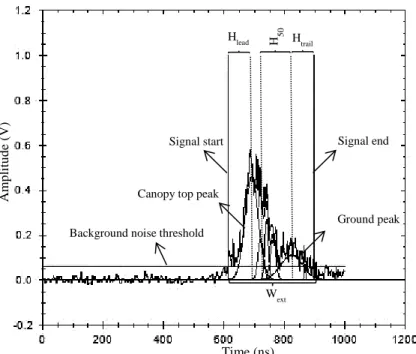
A collection of metrics were extracted or calculated from waveforms which were used as dependent variables later in estimating forest height and volume. Signal start and end are defined as first and last bins in the waveform where the waveform intensity exceeds background noise threshold, nσ+μ, where σ and μ recorded in GLA01 product are standard deviation and mean background noise respectively, and n=0.5,1,…,5. Different thresholds including 3σ+μ (Sun et al., 2008), 4σ+μ ([16]), 4.5σ+μ ([15], [17], [43]) were applied in previous studies. In [18] different thresholds were used for signal start and end for each three sites from 2.5σ+μ to 5σ+μ.
Hilbert & Schmullius [42] stated that the optimal thresholds might differ according to the waveform types, laser periods or footprint structure. In this research the threshold was set as 4.5σ+μ as optimum threshold in most studies.
The vertical distance between signal start and signal end of a waveform was computed as waveform extent (Wext) which could be affected by terrain slope, canopy height and canopy density ([44]). Since over complex terrain, last Gaussian peak cannot represent terrain elevation, the stronger one among two lowest Gaussian peaks was chosen as ground peak ([14], [15], [18], [25]). The first Gaussian peak was selected as canopy top. The distance between ground peak and signal start has been defined as maximum canopy height in flat area. The vertical distance from ground peak to signal end and from canopy top to signal start are defined as trail edge and lead edge extents, respectively ([15], [42]). H25, H50, H75 and H100 as quartile heights have been extracted from waveforms by calculating the vertical distance between ground peak and position of waveform at which respectively 25%, 50%, 75% and 100% of the returned energy between signal start and end occurs ([22], [32]). So the total waveform energy was calculated by summing all the return energies from signal start to end. Starting from the signal end, the position of the 25%, 50%, and 75% of energy were located by comparing the accumulated energy with total energy. H100 is the maximum canopy height as defined above. Fig. 3 illustrates a GLAS waveform from study area with Gaussian peaks and some extracted metrics. The metrics extracted from GLAS waveforms and their derivatives which were used in this research, are listed in Table. 2.
B. Height Estimation
It was aimed to find if GLAS/ICESat data are able to estimate maximum canopy height or Lorey’s height more accurate. To reach this goal, Lorey’s and maximum heights were calculated from field inventory data. Over flat area, estimation of maximum canopy height (Hmax) is based on vertical difference between the waveform signal start (Ss) and the ground peak (Gp) ([18]):
𝐻𝑚𝑎𝑥(𝑖𝑛 𝑚) = (𝐺𝑝 − 𝑆𝑠) × 0.15 (2)
Vertical resolution of waveforms is 15 cm (Harding & Carabajal, 2005).Over sloped terrain, peaks from ground and surface objects can be broadened and mixed, making identification of ground peak difficult ([16], [18], [24]). Hence it is necessary to find a way to decrease slope impact on waveform. Lefsky et al. [16] and Chen [18] used DEM to include topography effects on height estimations. Lefsky et al. [17] and Pang et al. [24] applied Hlead and Htrail extracted from waveforms to remove the broadening effects caused by the sloped terrain. In present research, Terrain Index (TI) was calculated using: 1) a fine resolution DEM (10 meters) produced based on 1:25000 topographic maps (called TI10); 2) SRTM DEM with 90 meter resolution (called TI90). The elevation range within a 7×7 neighborhood of 10m-DEM ([14], [18]) and 3×3 neighborhood of SRTM DEM ([15]) at
location of each GLAS footprint was considered as TI. The effect of using higher resolution DEM on model performance was investigated.
A large number of MLR and Random Forest (RF) models were developed employing different combination of metrics extracted from waveforms to predict maximum and Lorey’s height (e.g. [15], [17], [18], [24], [25]). It should be noted that RF consists of a large number of trees, created based on a random subset of observations and metrics. The overall prediction of the trees is calculated by averaging the predictions from the individual trees ([45], [46]).
As mentioned, the idea of using terrain index and edge extents came to remove the broadening effects of sloped terrain. It was questioned if other waveform metrics could improve the result. To answer this question, all metrics listed in Table. 2 were used as inputs to stepwise regression. It combines backward elimination and forward selection to reach best combination of metrics based on AIC criteria. This combination of metrics was used in both MLR and RF.
Principal Component Regressions (PCR) defined as a three step multivariate method including performing Principal Component Analysis (PCA); selection of relevant Principal Components (PCs); and MLR between selected PCs and response variable (canopy height or forest volume), was tested. PCA finds a set of synthetic variables (the principal components) that summarizes the original set. It rotates the axis of variation to give a new set of ordered orthogonal axis that summarizes describing proportions of the variations. In fact, the principal components (PCs) are uncorrelated and ordered such that the kth PC has the kth largest variance among all PCs ([47]). The traditional approach is to use the first few PCs in data analysis since they have most of the variation in the original data set. In this study, LiDAR signal intensities were used for the PCA analysis. In order to apply PCA, it is necessary to have equal number of samples in all waveforms. So, the length of largest waveform extent was considered as basis (400 samples) and other waveforms were apart from signal start toward signal end till the number of samples reach the base Wext’s samples. Since the number of observations (60) is less than the number of samples in the useful part of waveforms (400 samples), it was aimed to reduce the number of samples by selecting one among each ten samples. So PCA was performed using 41 samples as variables to find the main factors (waveform signals) determining most effects on forest canopy height ([25]). As it is seen in Table. 3, three first components have the most information, and explain 77.5% of variance in the data. MLR and RF regressions were developed using either all PCs or PCs from stepwise regression or three first PCs.
Wavelet-based Regressions (WR) were performed to estimate maximum and Lorey’s height. In wavelet transform, a signal with finite length (2n samples) is decomposed into two series: the first including the “father” wavelet coefficients describing overall variation and trend (smooth or low frequency part), and the second consisting of “mother” wavelet coefficients representing details (high frequency part) of the signal ([48], [49], [50]). Wavelet analysis was
performed to decompose waveforms using discrete wavelet transformation with the Haar wavelet function pair ([51]).
The necessity of having equal lengths of waveform extents made data preparation fundamental before wavelet analysis. So the same approach as PCA data preparation was performed to have 400 samples (the length of largest waveform extent) for each waveform. Since having limited number of observations (59), the policy of reducing waveform samples (400 samples) were employed three times by selecting one among 3, 6 or 11 samples. So, 134, 67 and 37 samples were kept, respectively. As the requisite sample size for wavelet transformation is a power of 2 (2n; n corresponds to the wavelet decomposition levels), 128 (27), 64 (26) and 32 (25) samples out of 134, 67 and 37 were used in analysis, respectively. Wavelet transformation on 128 samples (as example) produced 64, 32, 16, 8, 4, 2 and 1 coefficients from level 1 to level 7, respectively. Fig. 4 illustrates wavelet fit in 7 (128=27 samples), 6 (64=26 samples) and 5 levels (32=25 samples) for one waveform as instance. MLR and RF regressions were developed using either all Wavelet Coefficients (WCs) extracted from each level of decomposition or WCs after stepwise regression to estimate maximum and Lorey’s height. The number of coefficients of that level which is used in the regressions could not exceed the number of our observations (60).
C. Volume Estimation
Two methods were applied to estimate forest volume. The first method consists of three steps: 1) developing volume-Hmax and volume-HLorey relationships. The stronger one was chosen to estimate volume next. To find volume-height relationship, the common form used in different literatures ([15], [16], [20], [21], [26]), power relationship between V and canopy height (Refer to (3)), was used and calibrated based on our in situ data; 2) estimating height from GLAS data using best model resulted from subsection 3.2. It should be mentioned that if we choose volume-HLorey relationship at first step, Lorey’s height would be estimated form Lidar data; and 3) estimating forest volume (V) using chosen volume-height relationship. This method has been used in different studies like [15], [16], [21] and [26].
𝑉 = 𝑎 𝐻𝑏 (3)
Where H is Hmax or HLorey.
The second method estimates forest volume directly from GLAS waveforms ([29], [30], [32]). In fact a large number of MLR and RF regressions were developed based on waveform metrics or PCs or WCs to predict forest.
D. Model Validation
Twenty percent of observations were iteratively left out through a five-fold cross validation to validate developed models. A number of statistics was calculated between predicted parameter from GLAS data (maximum height, Lorey’s height or volume) and correspondent in situ measurements. Adjusted coefficient of determination (R2a.cv) as an indicator of the fit quality ([52]), Root Mean Square
Error (RMSE.cv) as a measure of accuracy ([43]), Mean Absolute Difference (MD.cv) as a measure of dispersion ([54]), Mean Absolute Percentage Error (MAPE) as an expression of accuracy in percentage ([55], [56]), and Akaike Information Criterion (AIC.cv) as a means for model selection by trading-off between the goodness of fit of the model and the complexity of the model ([41]) were used to evaluate the result of predictions.
IV. RESULTS AND DISCUSSION
A. Maximum Canopy Height Estimation
An objective of this study is predicting maximum canopy height in complex mountainous forests with significant slope. Since impossibility of extracting maximum height over steep area by calculating the difference between signal start and ground peak, lots of regression models were built. Table. 4 represents five models developed based on main metrics extracted from waveforms (Table. 1) and TI10. It contains a most accurate model (among all MLR and RF) along with some models having the most common metrics. As it seen an MLR model combined Wext2.5, Wext1.5, ln(H50) and TI101.5 (model 1) produced the lowest AIC.cv (296.3) and highest accuracy (5.0m). Based on the MAPE.cv, 16.4% of predictions of this model are off (Fig. 5a). The t-statistics of regression coefficients shows the relative importance of each metric in the model ([50]). Based on this statistics, TI101.5 and Wext1.5 contribute most to the model for this set of independent variables.
Worth to notice, the accuracy of simplest model in Table. 4 (6.3m) is more than one meter lower than first model (5.0m), as the best one. So the first model is preferable even if it needs more metrics to be extracted.
As it is seen in Fig. 5a, maximum canopy height has been over-estimated where there are short trees (height < 10m). Overestimation is expected especially where short trees are located over a sloped terrain. In these conditions, the elevation of the highest object within a footprint is not necessarily at the top of the tallest tree, and could be a shorter tree located in higher elevation or even terrain instead of any vegetation ([18]) which could be expected for sparse canopy over steep terrain. Deep investigation in our field data confirms footprints possessing short trees are located over a sloped terrain (the range of terrain slope for these footprints except one (20%) is between 40-55%) with low basal area as a proxy of forest density. However the problem of slope has been solved greatly using a regression model combining terrain information with GLAS’s waveform metrics, the overestimation in short-tree stands remains unresolved. This was also reported by Nelson [57]. He showed lack of efficiency of GLAS data to accurately measure forest structure in short-tree sparse forests.
Replacement the TI90 with TI10 in the model 1 led to an R2a.cv and RMSE.cv equal 0.81 and 5.6m, respectively (Fig. 5b). As it is seen the model with TI10 produced slightly better result. This is contrary to our expectations for producing much more accurate result using local DEM generated from topographic map rather than SRTM DEM. A reason could be
that conventional DEMs produced from photogrammetric techniques might not adequately characterize topography over forest areas ([58]). Conclusively, the SRTM DEM could be an acceptable source of information about terrain variability especially in large extent areas with presence of forest cover. Recent availability to the SRTM DEM30 for whole world (with more details rather than SRTM DEM90) strengthens this deduction.
Since obtaining similar outputs concerning DEM10 and SRTM DEM throughout our study, only results of models containing TI10 are discussed from here to the end.
Among RF regressions, the best result was obtained using metrics Wext2.5, Wext1.5, H50 and TI101.5 with an R2a.cv, RMSE.cv, MD.cv and MAPE.cv of 0.72, 6.9m, 5.4m and 28.0%, respectively (Fig. 6).
Among all types of regression models, models containing TI represented better result with smaller RMSE.cv. It could be deduced that TI as a representative of terrain slope had an important effect on estimating maximum canopy height over steep area.
MLR and RF regressions using all PCs or PCs from stepwise regression did not produce better result rather than those based on waveform metrics. Three first PCs, explaining 77.5% of data variance, showed most performance in our models. The smallest AIC.cv (301.1) among MLR models belongs to model combining three first PCs, Wext and TIt. It produced an R2a.cv and RMSE.cv of 0.77 and 6.0m, respectively, the MD.cv between predicted and observed height is about 4.7m, and the prediction error is about 22.1% (Refer to (4), Fig. 7a). The best result concerning RF regressions was generated using the same metrics (three first PCs, Wext and TI10) with an R2a.cv and RMSE.cv of 0.66 and 8.0m, respectively, MD.cv of 6.2m and the prediction error of about 36.0% (Refer to (5), Fig. 7b).
𝐻𝑚𝑎𝑥= 3.8289𝑃𝐶1+ 2.157𝑃𝐶2− 6.0618𝑃𝐶3+
1.2449𝑊𝑒𝑥𝑡− 0.4494𝑇𝐼10− 6.5857 (4)
𝐻𝑚𝑎𝑥= 𝑅𝐹(𝑃𝐶1, 𝑃𝐶2, 𝑃𝐶3, 𝑊𝑒𝑥𝑡, 𝑇𝐼10 ) (5)
In RF regressions, according to random sampling of observations, about one third of the observations are not used for any individual tree which is called Out of Bag (OOB) for that tree ([45], [46]). The variable importance is determined by how much worse the OOB predictions of random forest can be if the data for that variable are randomly permuted. In fact, it would be possible to find out what would happen with or without the help of that variable. Variable importance measures produced by random forest can also sometimes be useful to build simpler model ([59], [60]). In RF regression of Eq. 5, Wext has the highest importance, and subsequently has the main roll in strength of the model and TI10 is in the third level of importance after Wext and PC3. PC3 and PC2 have in turn more importance rather than PC1. Although PC1 has the most variance among all PCs, it is less correlated to dependent variable (height) rather than second and third PCs. This confirms that the informative part of waveform is not always
in the first PC.
The same approach of PCR was performed in WR. In other word, WCs at different level of decompositions along with two important metrics, Wext and TI10 were entered in MLR and RF models to predict maximum height. The best result was obtained by WCs extracted from first level of waveform decomposition including 32 samples. An MLR model (Refer to (6), Fig. 8a) combining Wext, TI10 and five WCs determined by stepwise regression of first level coefficients (16 WCs), produced lowest AIC.cv (317.2) and greatest accuracy (R2a.cv = 0.73, RMSE.cv = 6.5m, MD.cv = 5.5m, MAPE.cv = 22.6%). Among RF regressions, highest accuracy was resulted from the same combination of metrics in Eq.6, with an R2a.cv of 0.71, RMSE.cv of 7.8m, MD.cv of 6.2m and MAPE.cv of 34.5% (Refer to (7), Fig. 8b).
𝐻𝑚𝑎𝑥= 20.1791𝑊𝐶2+ 10.7454𝑊𝐶3+ 0.9372𝑊𝐶5−
42.1402𝑊𝐶13+ 5.7257𝑊𝐶16+ 1.08544𝑊𝑒𝑥𝑡−
0.4343𝑇𝐼10− 2.2611 (6)
𝐻𝑚𝑎𝑥= 𝑅𝐹(𝑊𝐶2, 𝑊𝐶3, 𝑊𝐶5, 𝑊𝐶13, 𝑊𝐶16, 𝑊𝑒𝑥𝑡, 𝑇𝐼10) (7)
As a conclusion, it is possible to estimate maximum height from GLAS data with an accuracy of about 5 m over significant sloped area with a simple MLR model based on a combination of H50 and derivatives of Wext and TI10. Chen [18] estimated maximum height in three study sites Mendocino, Santa Clara and Lewis with an accuracy of 6.18m, 4.88m and 9.31m, respectively, using a linear model of Wext and TI10. While these sites are similar in slope (average slope of 20 degrees), they are different in case of forest type. It worth to notice that there is lower canopy cover and smaller trees in Santa Clara rather than two other sites. It could be deduced that while slope is a very important factor affecting height estimation, other properties of forest (forest type, forest vertical and horizontal structure) should be considered too. So it could be interesting if we classify our data into different kinds of classes and analyze them separately. Since limited number of field observations in our study, it was not possible to have such analysis.
B. Lorey’s Height Estimation
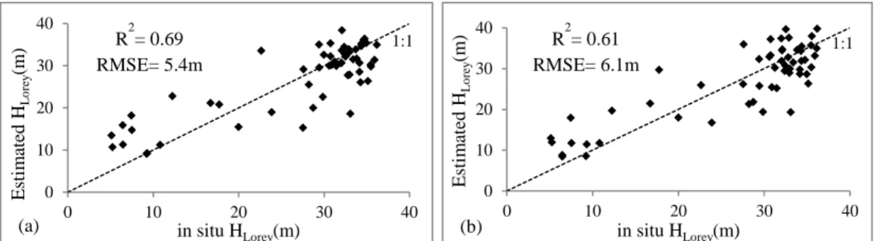
It was aimed to see how accurate would be Lorey’s height predicted from GLAS data and how much the predictions are better rather than maximum height estimated from GLAS data. Totally, MLR models produced better accuracy rather than RF regressions in all combination of metrics including waveform metrics, PCs and WCs. This has been observed also for maximum height estimations in section 4.1. So only the result of MLR models is presented in this section. Table. 5 represents a most accurate model (model 1) and four other models based on most common metrics. The MLR model including ln(Wext) and TI10 produced lowest AIC.cv (288.3) with a prediction error of about 24.0% and RMSE.cv of 5.1m (Fig. 9).
Equations (8) and (9) represent the best models using PCR and WR, respectively. For PCR, lowest AIC.cv (304.9) was
observed in an MLR model including three first PCs, Wext and TI10 (R2a.cv= 0.66, RMSE.cv= 5.4m, MD.cv= 4.0m, MAPE= 24.1%). For WR, an MLR based on WCs extracted from first level of waveform decomposition (including 32 samples), produced lowest AIC.cv (310.9). This model is combined of Wext, TI10 and six out of sixteen WCs determined by stepwise regression of first level coefficients (R2a.cv= 0.55, RMSE.cv= 6.1m, MD.cv= 4.6m, MAPE= 28.0%). Fig. 10a and 10b represent Lorey’s height estimated from PCR and WR.
𝐻𝐿𝑜𝑟𝑒𝑦= −4.5647𝑃𝐶1− 0.2831𝑃𝐶2+ 1.5421𝑃𝐶3+
0.9006𝑊𝑒𝑥𝑡− 0.30802𝑇𝐼10− 4.4943 (8)
𝐻𝐿𝑜𝑟𝑒𝑦= 26.95035𝑊𝐶2− 7.173𝑊𝐶3+ 7.260𝑊𝐶5−
9.140𝑊𝐶8− 57.6514𝑊𝐶13− 12.6797𝑊𝐶16+
0.7078𝑊𝑒𝑥𝑡− 0.10713𝑇𝐼10+ 1.28 (9)
As it is observed, the accuracy of Lorey’s height estimation using MLR based on waveform metrics is approximately equal to that for maximum height (around 5m). But worth considering point is using a simpler model to predict Lorey’s height rather than maximum height. Regards to PCR and WR, the accuracy of Lorey’s height prediction is lower than models based on waveform metrics but it is higher in comparison with those calculated for maximum height predictions.
C. Forest Volume Estimation
1) Volume Estimation using Volume-Lorey’s Height Relationship The objective was to estimate volume using height predicted from GLAS data. To reach this, volume-height relationships were developed based on in situ measurements. Since volume showed stronger relationship to Lorey’s height rather than maximum height, the developed volume-HLorey model was chosen to predict forest volume (Refer to (10)). Fig. 11 represents the relationship between in situ volume and both maximum and Lorey’s height.
𝑉 = 2.6507 𝐻𝐿𝑜𝑟𝑒𝑦1.5434 (10)
Lorey’s height estimated using model 1 of Table. 5, as the best model among all types of regressions (MLR and RF using waveform metrics, PCs and WCs), was entered in volume-height relationship as independent variable. Comparison of estimated and measured volume produced an R2a and RMSE of 0.51 and 167.8 m3/ha, respectively.
There are several sources of error that resulted propagation of error and low accuracy of volume estimation. Two main sources could be: 1) height-DBH relationships used to estimate height of all trees in each plot to compute Lorey’s height; 2) it is known that forest volume is a function of height and diameter as two essential quantitative factors. Since with lidar data, only third dimension of objects could be retrieved, volume-height relationship was developed with an RMSE and R2a of 106.6 m3/ha and 0.80, respectively (Fig. 7). Even using accurate ground measured height; the accuracy of volume estimated based on above relationship is greater than 100 m3/ha. So this relationship could not be reliable enough to
estimate volume based on Lorey’s height extracted from GLAS data. Deep investigation in field inventory data shows the possibility of having same Lorey’s height for completely different forest structure which leads to different forest volume. To better understanding, three couple of plots have been compared in Table. 6 concerning Lorey’s height (m), number of trees (n/ha) and volume (m3/ha). As it is seen, plots with approximately the same Lorey’s height have different volume. It approves that estimating forest volume only relying on an average height could cause a high discrepancy with reality especially in uneven aged forests.
2) Volume estimation directly from GLAS data
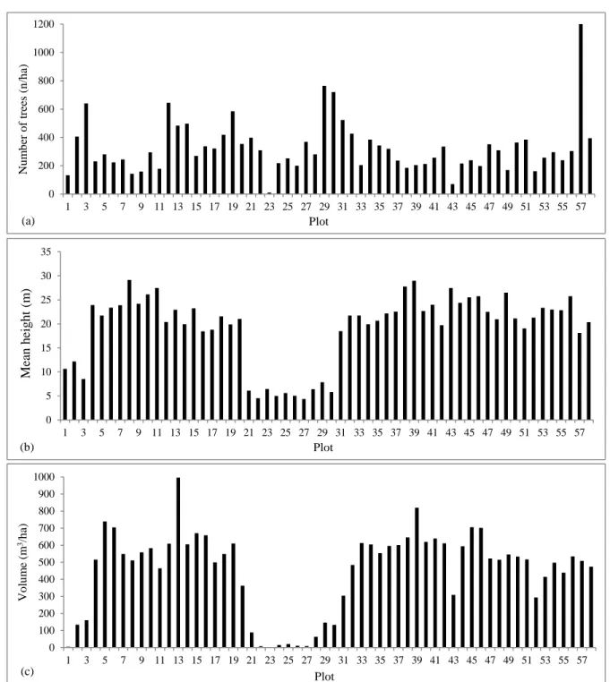
It was under question whether the result of volume estimation would improve if we extract that directly from GLAS data instead of using volume-Lorey’s height relationship. So a large number of MLR and RF models were developed to estimate forest volume from waveform metrics, PCs or WCs to overcome the extra errors resulted from height-DBH and volume-height relationships mentioned in section 4.3.1. The best result was observed using MLR models based on waveform metrics. As it is seen in Table. 7, lowest AIC.cv (595.1) was produced using model 2 with an accuracy of 137.0 m. Since the difference between AIC of the first model (597.0) and the minimum AIC (595.1) is less than 2, the model 1 could have a substantial support ([41], [18]). This model (model 1 in Table. 7, Fig. 12) produced better accuracy (128.8 m), but it is still not satisfying. It could be because of other factors besides height affecting volume like DBH and number of trees per hectare while all metrics in model 1 (Table. 7) are related to height. By the way the heterogeneity of forest may decrease the ability of LiDAR data to estimate forest volume. As it is seen in Fig. 13c, there are plots with very low volume (plots 22-27) and also with very high volume (plot 13). It is expected to have higher accuracies in homogenous forests. On the other hand, comparison of different plots in Fig. 13 demonstrates dependency of volume to diverse factors. In other word, it happens to have high number of trees per hectare but low volume and reverse, equal number of trees per hectare or equal mean height but different volume. So it is expected to improve the result of LiDAR estimation by finding waveform metrics representative of other factors like DBH and forest density, in addition to forest height, affecting forest volume. Nelson et al. [32] predicted timber volume with an R2a of 0.75 and RMSE of 87 m3/ha using a neural network model employing six different metrics extracted from waveform metrics (h̄med: a median height which below that cumulative canopy height profile (CHP) is 50% at maximum; h2-sun: a corrected maximum height; hg1-sun: height of waveform peak with the maximum amplitude above ground peak, f: the slope of the line formed by connecting the signal start point with the peak of the uppermost Gaussian return, rg3: the waveform area under the 3rd Gaussian peak, and ng:the number of Gaussian peaks in the waveform). This raises the question whether using the same methodology and metrics of Nelson et al. [32] could enhance the result in our study area. Although forest properties including forest type, horizontal
and vertical structure and topographical properties could affect the results.
MLR and RF regressions using PCs and WCs did not show better performance in comparison with those using waveform metrics. The best PCR model was an MLR combining three first PCs, Wext and TI10 (R2a= 0.67, RMSE= 131.5 m3/ha). The highest accuracy concerning WR was obtained using WCs extracted from second level (32 WCs) of waveform decomposition including 128 samples. In fact an MLR model combining Wext, TI10 and five out of thirty two WCs (determined by stepwise regression) produced an accuracy of 140.3 m3/ha.
As the results show, estimating forest volume directly from GLAS data reduces the errors, and leads to higher accuracy. But it is still under consideration to approach a method enhancing the result.
V. CONCLUSION
This research contains three main parts and aims to investigate the capability of GLAS data in estimating maximum canopy height (Hmax), Lorey’s height (HLorey) and forest volume (V). Numerous MLR and RF regressions were developed using different set of metrics including waveform metrics, PCs and WCs to estimate each parameter. Concerning Hmax, an MLR model based on waveform metrics produced the greatest accuracy (5.0 m). PCs and WCs based models were not able to predict the Hmax with accuracy better than 6 m. Also totally, MLR models represented better performance rather than RF regressions in this study. These results are in contrast with Fayad et al. [25] that observed approximately the same accuracies in predicting canopy height using MLR or RF models, also waveform metrics or PCs based models. This confirms the local applicability of fitted regressions. The important point regards study of Fayad et al. [25] is terrain topography which is mostly flat and sometimes with low slope (slope < 15˚).
Concerning HLorey, a simpler MLR model including Wext and TI resulted in an accuracy of 5.1m which is slightly better than PCs based model (5.4m), but with accuracy about 1 meter greater than WCs based model. Furthermore better performance was observed using MLR in comparison with RF regressions.
In total, two metrics, Wext and TI, showed great importance in height and volume predictions. These metrics also enhanced the performance of PCR and WR, greatly. Since two sources of DEM were available to extract TI10 and TI90, the analysis was performed based on both. However the result of models using TI10 is better than those using TI90, but it does not discourage the importance of SRTM DEM especially with current availability to the SRTM DEM30 for whole world. It is expected to reach higher accuracy using DEM derived from airborne lidar data which has been confirmed in [18].
Regards to volume predictions, two approaches were considered. The first, estimates volume using volume-height relationship and the second do predictions using regressions developed between in situ volume and lidar based metrics. Based on our result, an MLR model including waveform
metrics would predict forest volume with an accuracy of about 128m. Although the result is a little better in comparison with volume estimated from volume-height relationship (as a reason of absence of some sources of error mentioned in section 4.3.1), the result is still not satisfying. It raised the question whether using other methods of analysis like Support Vector Machine (SVM) and Artificial Neural Network (ANN), or using combination of radar, lidar, optical images and complementary data like meteorological, geological and forest type map will enhance the accuracy of forest volume estimation. These questions will be considered and discussed in a future study.
There are general sources of uncertainty in predicting forest biophysical parameters: 1) Time interval between Lidar data acquisition and field measurements; 2) measurement uncertainty especially about height quantity which is dependent on measuring tool, the measurement procedure, the skill of the operator, the environment, and other effects; 3) in situ volume which is not a true value measured for each tree but an estimated value from volume-height-diameter relationships; 4) probability of error in ground peak identification from lidar waveforms especially in sloped area. Identification of ground peak is essential for extracting some waveform metrics like trail edge extent and height at quarters of returned signal energy; 5) uncertainty in locating GLAS footprints on the ground correctly. It should be noted that small number of observations, i.e. 60 ground plots covering whole study area with a diverse structure, is a limitation of this study. It would be desirable to first classify the forest into different classes (forest type and forest density), then perform analysis in each class which requires more observations covering the entire study site.
ACKNOWLEDGEMENT
Many thanks are extended to Iran National Science Foundation (INSF) and also an international joint PhD program, “Cotutelle”, initiated by France for financial support of this research. Thanks are also extended to the members of forest research station of Nowshahr for their collaboration in gathering field measurements and providing required equipment.
REFERENCES
[1] H. D. Vance-Chalcraft, M. R. Willig, S. B. Cox, A. E. Lugo & F. N. Scatena, “Relationship between aboveground biomass and multiple measures of biodiversity in subtropical forest of puerto rico,” Biotropica, vol. 42, no. 3, pp. 290-299, 2010
[2] J. R. Lasky, M. Uriarte, V. K. Boukili, D. L. Erickson, W. J. Kress & R. L. Chazdon, “The relationship between tree biodiversity and biomass dynamics changes with tropical forest succession,” Ecol. Lett., vol. 17, pp. 1158-1167, 2014.
[3] S. P. Hamburg, D. G. Zamolodchikov, G. N. Korovin, V. V. Nefedjev, A. I. Utkin, J. I. Gulbe & T. A. Gulbe, “Estimating the carbon content of Russian forests: a comparison of phytomass/volume and allometric projections,” Mitigation Adapt. Strateg. Glob. Chang., vol. 2, pp. 247-265, 1997.
[4] H. Ding, P. A. L. D. Nunes & S. “Teelucksingh, European forests and carbon sequestration services: an economic assessment of climate change impacts,” ESE, UNEP, No. 9, Jan. 2011.
[5] X. Cheng, M. Yu & T. Wu, “Eeffect of forest structural change on carbon storage in a coastal metasequoia glyptostroboides stand,” The
Scientific World Journal, vol. 830509, pp. 1-9, 2013.
[6] M. Macauley, D. Morris, R. Sedjo, K. Farley & B. Sohngen, “Forest Measurement and Monitoring: Technical Capacity and How Good Is Good Enough?,” Washington DC: Resources for the Future, Dec. 2009. [7] Namiranian, M., Measurement of Tree and Forest Biometry, 1st Edition,
Tehran University Publications, ISBN: 964-03-5439-2, 2007, 574pp (In Persian).
[8] H. T. Schreuder, T. G. Gregoire & G. B. Wood, “Mensurational aspects of forest inventory,” in Sampling Methods for Multiresource Forest
Inventory, New York, Wiley, 1993, pp. 227-315.
[9] D. R. Miller, Ch. P. Quineb & W. Hadley, “An investigation of the potential of digital photogrammetry to provide measurements of forest characteristics and abiotic damage,” For. Ecol. Manage., vol. 135, pp. 279-288, 2000.
[10] T. Gobakken, O. M. Bollandsås & E. Næsset, “Comparing biophysical forest characteristics estimated from photogrammetric matching of aerial images and airborne laser scanning data,” Scand. J. For. Res., vol. 30, no. 1, pp. 73-86, 2015.
[11] H. Balzter, C. S. Rowland & P. Saich, “Forest canopy height and carbon estimation at Monks Wood National Nature Reserve, UK, using dual-wavelength SAR interferometry,” Remote Sens. Environ., vol. 108, pp. 224-239, 2007.
[12] S. Attarchi & R. Gloaguen, “Improving the estimation of above ground biomass using dual polarimetric palsar and ETM+ data in the Hyrcanian mountain forest (Iran),” Remote Sens., vol. 6, pp. 3693-3715, 2014. [13] S. Aronoff, “Active sensors: Radar and Lidar,” in Remote Sensing for
GIS Managers, ESRI Press, 2005, 487 pp.
[14] J. A. B. Rosette, P. R. J. North & J. C. Suarez, “Vegetation height estimates for a mixed temperate forest using satellite laser altimetry,”
Int. J. Remote Sens., vol. 29, no. 5, pp. 1475-1493, 2008.
[15] N. Baghdadi, G. Maire, I. Fayad, J. S. Bailly, Y. Nouvellon, C. Lemos & R. Hakamada, “Testing different methods of forest height and aboveground biomass estimations from ICESat/GLAS data in Eucalyptus plantations in Brazil,” IEEE JSTARS, vol. 7, no. 1, pp. 290-299, 2014.
[16] M. A. Lefsky, D. J. Harding, M. Keller, W. B. Cohen, C. C. Carabajal, F. D. Espirito-Santo, M. O. Hunter, R. de Oliveira & P. B. de Camargo, “Estimates of forest canopy height and aboveground biomass using lCESat,” Geophys. Res. Lett., vol. 32, no. 22, pp. 1-4, 2005.
[17] M. A. Lefsky, M. Keller, Y. Pang, P. B. de Camargo & M. O. Hunter, “Revised method for forest canopy height estimation from Geoscience Laser Altimeter System waveform,” J. Appl. Remote Sens., vol. 1, pp. 1-18, 2007.
[18] Q. Chen, “Retrieving vegetation height of forests and woodlands over mountainous areas in the Pacific Coast region using satellite laser altimetry,” Remote Sens. Environ., vol. 114, pp. 1610-1627, 2010. [19] L. I. Duncanson, K. O. Niemann & M. A. Wulder, “Estimating forest
canopy height and terrain relief from GLAS waveform metrics,” Remote
Sens. Environ., vol. 114, pp. 138-154, 2010.
[20] S. S. Saatchi, H. L., S. Brown, M. Lefsky, E. T. Mitchard, W. Salas, B. R. Zutta, W. Buermann, S. L. Lewis, S. Hagen, S. Petrova, L. White, M. Silman & A. Morel, “Benchmark map of forest carbon stocks in tropical regions across three continents,” Proc Natl Acad Sci USA, vol. 108, no. 2, pp. 9899-9904, 2011.
[21] E. T. A. Mitchard, S. S. Saatchi, L. J. T. White, K. A. Abernethy, K. J. Jeffery, S. L. Lewis, M. Collins, M. A. Lefsky, M. E. Leal, I. H. Woodhouse & P. Meir, “Mapping tropical forest biomass with radar and spaceborne LiDAR in Lop´e National Park, Gabon: overcoming problems of high biomass and persistent cloud,” Biogeosciences, vol. 9, pp. 179-191, 2012.
[22] G. Sun, K. J. Ranson, D. S. Kimes, J. B. Blair & K. Kovacs, “Forest vertical structure from GLAS: An evaluation using LVIS and SRTM data,” Remote Sens. Environ., vol. 112, pp. 107-117, 2008.
[23] Y. Xing, A. de Gier, J. Zhang & L. Wang, “An improved method for estimating forest canopy height using ICESat-GLAS full waveform data over sloping terrain: A case study in Changbai mountains, China,” Int. J.
Appl. Earth Obs. Geoinf., vol. 12, pp. 385-392, 2010.
[24] Y. Pang, M. Lefsky, G. Sun, M. Ellen Miller & Z. Li, Temperate forest height estimation performance using ICESat GLAS data from different observation periods, IAPRS, Vol. XXXVII, Part B7, pp. 777-782, 2008. [25] I. Fayad, N. Baghdadi, J-S. Bailly, N. Barbier, V. Gond, M. El Hajj, F.
Fabre & B. Bourgine, “Canopy height estimation in French Guiana with LiDAR ICESat/GLAS data using principal component analysis and
random forest regressions,” Remote Sens., vol. 6, pp. 11883-11914, 2014.
[26] S. P. Healey, P. L. Patterson, S. Saatchi, M. A. Lefsky, A. J. Lister & E. A. Freeman, “Sample design for globally consistent biomass estimation using lidar data from the Geoscience Laser Altimeter System (GLAS),”
Carbon Balance Manag., vol. 7, pp. 1-10, 2012.
[27] G. P. Asner & J. Mascaro, “Mapping tropical forest carbon: Calibrating plot estimates to a simple LiDAR metric,” Remote Sens. Environ., vol. 140, pp. 614-624, 2014.
[28] J. Boudreau, R. F. Nelson, H. A. Margolis, A. Beaudoin, L. Guindon & D. S. Kimes, “Regional aboveground forest biomass using airborne and spaceborne LiDAR in Québec,” Remote Sens. Environ., vol. 112, pp. 3876-3890, 2008.
[29] L. I. Duncanson, “Aboveground biomass estimation using spaceborne LiDAR in managed conifer forests in south central British Columbia,” M.S. thesis, Dept. Geography, Univ. Victoria, 2009.
[30] G. Zhifeng, CH. Hong & S. Guoqing, “Estimating forest aboveground biomass using HJ-1 satellite CCD and ICESat GLAS waveform data,”
Science China Earth Sciences, vol. 53, no. 1, pp. 16-25, 2010.
[31] A. Fu, S. Guoqing & G. Zhifeng, “Estimating forest biomass with GLAS samples and MODIS imagery in northeastern China,” Proc. SPIE., 2009, Vol. 7498: pp. 1-8.
[32] R. Nelson, K.J. Ranson, G. Sun, D.S. Kimes, V. Kharuk & P. Montesano, “Estimating Siberian timber volume using MODIS and ICESat/GLAS,” Remote Sens. Environ., vol. 113, pp. 691-701, 2009. [33] M. Quiñones, D. H. Hoekman, V. Schut & N. Wielaard, “Above ground
biomass map of Kalimantan,” SarVision, Germany, Rep. 80087-SV-BMU, Nov. 2011.
[34] A. G. Brenner, R. J. Zwally, C. R. Bentley, B. M. Csatho, D. J. Harding, M. A. Hofton, J. B. Minster, L. Roberts, J. L. Saba, R. R. Thomas & D. Yi3, “Derivation of range and range distributions from laser pulse waveform analysis for surface elevations, roughness, slope, and vegetation heights, Geoscience Laser Altimeter System (GLAS),” Version 4.1, Algorithm theoretical basis document, NASA’s EOS, Sep. 2003.
[35] D. J. Harding & C.C. Carabajal, “ICESat waveform measurements of within-footprint topographic relief and vegetation vertical structure,”
Geophys. Res. Lett., vol. 32, L21S10, 2005.
[36] S. Huang, S. J. Titus & D. P. Wiens, “Comparison of nonlinear height-diameter functions for major Alberta tree species,” Can. J. For. Res., vol. 22, pp. 1297-1304, 1992.
[37] J. L. Batista, H. T. Z. Couto & M. Marquesini, “Performance of height-diameter relationship models: analysis in three forest types,” Scientia
Forestalis, vol. 60, pp. 149-163, 2001.
[38] Z. Fang & R. L. Bailey, “Height-diameter models for tropical forests on Hainan Island in southern China,” For. Ecol. Manage., vol. 110, pp. 315-327, 1998.
[39] M. A. Silva Scaranello, L. F. Alves, S. A. Vieira, P. B. Camargo, C. A. Joly & L. A. Martinelli, “Height-diameter relationships of tropical Atlantic moist forest trees in southeastern Brazil,” Scientia Agricola, vol. 69, no. 1, pp. 26-37, 2012.
[40] K. Ahmadi, S. J. Alavi, M. T. Kouchaksaraei & W. Aertsen, “Non-linear height-diameter models for oriental beech (Fagus orientalis Lipsky) in the Hyrcanian forests, Iran,” Biotechnol. Agron. Soc. Environ., vol. 17, no. 3, pp. 431-440, 2013.
[41] K.P. Burnham & D. R. Anderson, “Information and likelihood theory: a basis for model selection and inference,” in Model Selection and
Multimodel Inference: A Practical Information-Theoretic Approach, 2nd
ed. New York: Springer-Verlag Press, 2002, pp. 49-97.
[42] C. Hilbert & Ch. Schmullius, “Influence of surface topography on ICESat/GLAS forest height estimation and waveform shape,” Remote
Sens., vol. 4, pp. 2210-2235, 2012.
[43] S. Lee, W. Ni-Meister, W. Yang & Q. Chen, “Physically based vertical vegetation structure retrieval from ICESat data: validation using LVIS in White Mountain national forest, New Hampshire, USA,” Remote Sens.
Environ., vol. 115, pp. 2776-2785, 2011.
[44] W. Yang, W. Ni-Meister & Sh. Lee, “Assessment of the impacts of surface topography, off-nadir pointing and vegetation structure on vegetation lidar waveforms using an extended geometric optical and radiative transfer model,” Remote Sens. Environ., vol. 115, pp. 2810-2822, 2011.
[45] L. Breiman, “Random Forests,” Machine Learning, vol. 45, pp. 5-32, 2001.
[46] U., Grömping, “Variable importance assessment in regression: linear regression versus random forest,” The American Statistician, vol. 63, no. 4, pp. 308-319, 2009.
[47] M. O. Ulfarsson, “Model based principal component analysis with application to functional magnetic resonance imaging,” Ph.D. dissertation, Dept. Electrical Engineering: Systems, Univ. Michigan, 2007.
[48] B. K. Alsberg, A. M. Woodward, M. K. Winson, J. J. Rowland & D. B. Kell, “Variable selection in wavelet regression models,” Analytica
Chimica Acta, vol. 368, pp. 29-44, 1998.
[49] G. Carl & I. Kühn, “Analyzing spatial ecological data using linear regression and wavelet analysis,” Stoch Environ Res Risk Assess., vol. 22, pp. 315-324, 2008.
[50] X. F. Wei, “Wavelet analysis for aboveground biomass estimate in temperate deciduous forests,” Ph.D. dissertation, Indiana State University, U.S., 2008.
[51] B. Whitcher, “Basic wavelet routines for one-, two- and three-dimensional signal processing, Package ‘waveslim’,” CRAN: The Comprehensive R Archive Network, pp. 1-81, 2014.
[52] A. C. Cameron & F. A. G. Windmeijer, “R-Squared measures for count data regression models wwith applications to health care utilization,” J. Bus. Econ. Stat., pp. 1-35, 1995.
[53] T. Chai & R. R. Draxler, “Root mean square error (RMSE) or mean absolute error (MAE)? -Arguments against avoiding RMSE in the literature,” Geosci. Model Dev., vol. 7, pp. 1247-1250, 2014.
[54] C. J. Willmott & K. Matsuura, “Advantages of the mean absolute error (MAE) over the root mean square error (RMSE) in assessing average model performance,” Clim. Res., vol. 30, pp. 79-82, 2005.
[55] S. Makridakis & M. Hibon, “Evaluating Accuracy (or Error) Measures,” INSEAD, Fontainebleau, France, 1995.
[56] R. J. Hyndman & A. B. Koehler, “Another Look at Measures of Forecast Accuracy,” Dept. Eco. and Bus. Statistics Monash Univ., Australia, ISSN 1440-771X, 2005.
[57] R. Nelson, “Model effects on GLAS-based regional estimates of forest biomass and carbon,” Int. J. Remote Sens., vol. 31, no. 5, pp. 1359-1372, 2010.
[58] Lidar 101: An Introduction to Lidar Technology, Data, and
Applications, Revised. Charleston, SC: NOAA Coastal Services Center,
2012.
[59] A. Liaw & M. Wiener, “Classification and regression by random forest,”
R News, vol. 2, no. 3, pp. 18- 22, 2002.
[60] Ch. L. Wei, G. T. Rowe, E. Escobar-Briones, A. Boetius, T. Soltwedel, M.J. Caley, Y. Soliman, F. Huettmann, F. Qu, Z. Yu, C.R. Pitcher, R.L. Haedrich, M.K. Wicksten, M.A. Rex, J.G. Baguley, J. Sharma, R. Danovaro, I.R. MacDonald, C.C. Nunnally, J.W. Deming, P. Montagna, M. Le´vesque, J.M. Weslawski, M. Wlodarska-Kowalczuk, B.S. Ingole, B.J. Bett, D.S.M. Billett, A. Yool, B.A. Bluhm, K. Iken & B.E. Narayanaswamy, 2010. “Global patterns and predictions of seafloor biomass using random forests,” PLoS ONE, vol. 5, no. 12, pp. 1-15.
Fig. 1. (a): Location of study area in Iran (red point) and its magnified view on a Landsat image (red border);( b): GLAS/ICESat-orbits, L3K and L3I, over a hillshade image (right) for the area indicated by a blue box on the left image.
Fig. 2. Overview of forest canopy height and volume estimation Field measurement
DBH
Height-DBH relationship
Height calculated for all trees
HLorey Volume-HLorey relationship Estimated Volume (1) Volume Maximum Height (Hmax) DEM10 Extract Terrain Index
GLAS data Filtering footprints High quality GLAS footprints Waveform metrics PCs of PCA WCs of WT DEM90 MLR and RF regressions and 5-fold cross validation
Estimated Hmax Estimated HLorey Estimated Volume (2) Volume-Hmax relationship
Fig. 3. A GLAS waveform and some metrics over a terrain of 25% slope in the study area. 1ns corresponds to 15 cm sampling distance in waveform.
Fig. 4. Wavelet fit in (a): 7 (128=27 samples), (b): 6 (64=26 samples) and (3): 5 levels (32=25 samples) for one waveform L2 L3 L4 L5 L6 L1 (b) L2 L3 L4 L5 L6 L7 L1 (a) L2 L3 L4 L5 L1 (c) Htrail Hlead H 50 Time (ns) Am p li tu d e (V) Signal end Ground peak Wext Signal start
Canopy top peak
Fig. 5. Maximum height estimated (m) from GLAS data based on waveform metrics and TI versus in situ maximum height (m). TI extracted from DEM10 (a) or DEM90 (b).
Fig. 6. Maximum height estimated (m) from GLAS data based on waveform metrics and TI10 versus in situ maximum height (m) using RF regression.
Fig 7. Maximum height estimated (m) based on PCs, Wext and TI10 using MLR: Eq. 4 (a) and RF regression: Eq. 5 (b) versus in situ maximum height (m).
Fig. 8. Maximum height estimated (m) based on WCs, Wext and TI10 using MLR: Eq. 6 (a) and RF regression: Eq. 7 (b) versus in situ maximum height (m).
0 10 20 30 40 50 60 0 10 20 30 40 50 60 Esti m ated H m ax (m ) in situ Hmax(m) R2= 0.82 RMSE= 5.60 m 1:1 (b) 0 10 20 30 40 50 60 0 10 20 30 40 50 60 Estim ate d H m ax (m ) in situ Hmax(m) R2= 0.86 RMSE= 4.99 m 1:1 (a) 0 10 20 30 40 50 60 0 10 20 30 40 50 60 Esti m ated H m ax (m ) in situ Hmax(m) R2= 0.72 RMSE= 6.9m 1:1 0 10 20 30 40 50 60 0 10 20 30 40 50 60 Esti m ated H m ax (m ) in situ Hmax(m) 1:1 (a) R2= 0.79 RMSE= 6.0m 0 10 20 30 40 50 60 0 10 20 30 40 50 60 Esti m ated H m ax (m ) in situ Hmax(m) 1:1 (b) R2= 0.69 RMSE= 8.0m 0 10 20 30 40 50 60 0 10 20 30 40 50 60 Esti m ated H m ax (m ) in situ Hmax(m) 1:1 (a) R2= 0.76 RMSE= 6.5m 0 10 20 30 40 50 60 0 10 20 30 40 50 60 Esti m ated H m ax (m ) in situ Hmax(m) 1:1 (b) R2= 0.74 RMSE= 7.7m
Fig. 9. Lorey’s height estimated (m) waveform metrics and TI10 using model 1 (Table 5) versus in situ Lorey’s height (m).
Fig. 10. Lorey’s height estimated (m) based on PCs (a) and WCs (b) versus in situ Lorey’s height (m).
Fig. 11. In situ volume versus maximum height (a) and Lorey’s height (b).
Fig. 12. Estimated forest volume (m3/ha) based on waveform metrics (model 1, Table 7) versus in situ volume (m3/ha).
0 10 20 30 40 0 10 20 30 40 Esti m ated H L o re y (m ) in situ HLorey(m) 1:1 R2= 0.72 RMSE= 5.1m 0 10 20 30 40 0 10 20 30 40 Esti m ated H L o re y (m ) in situ HLorey(m) 1:1 R2= 0.61 RMSE= 6.1m (b) 0 10 20 30 40 0 10 20 30 40 Esti m ated H L o re y (m ) in situ HLorey(m) 1:1 (a) R2= 0.69 RMSE= 5.4m y = 2.594x1.427 R² = 0.75 RMSE= 118.58 m3/ha 0 200 400 600 800 1000 0 10 20 30 40 50 60 V o lu m e (m 3/h a) Hmax (m) (a) y = 2.6507x1.5434 R² = 0.80 RMSE=106.55 m3/ha 0 200 400 600 800 1000 0 10 20 30 40 V o lu m e (m 3/h a) HLorey (m) (b) 0 200 400 600 800 1000 0 200 400 600 800 1000 Est imat ed v o lu me ( m 3/h a)
in situ volume (m3/ha)
1:1
R2= 0.71 RMSE= 128.8m3/ha
Fig. 13. (a): Distribution of number of trees (n/ha), (b): Mean height (m) and (c): forest volume (m3/ha) in 58 plots 0 200 400 600 800 1000 1200 1 3 5 7 9 11 13 15 17 19 21 23 25 27 29 31 33 35 37 39 41 43 45 47 49 51 53 55 57 Nu m b er o f tree s (n /h a) Plot (a) 0 5 10 15 20 25 30 35 1 3 5 7 9 11 13 15 17 19 21 23 25 27 29 31 33 35 37 39 41 43 45 47 49 51 53 55 57 Me an h eig h t (m ) Plot (b) 0 100 200 300 400 500 600 700 800 900 1000 1 3 5 7 9 11 13 15 17 19 21 23 25 27 29 31 33 35 37 39 41 43 45 47 49 51 53 55 57 V o lu m e (m 3/h a) Plot (c)