How large are present-day heat flux variations across the surface of Mars?

(1)

HAL Id: hal-02458627

https://hal.archives-ouvertes.fr/hal-02458627

Submitted on 26 Jun 2020

HAL is a multi-disciplinary open access

archive for the deposit and dissemination of

sci-entific research documents, whether they are

pub-lished or not. The documents may come from

teaching and research institutions in France or

abroad, or from public or private research centers.

L’archive ouverte pluridisciplinaire HAL, est

destinée au dépôt et à la diffusion de documents

scientifiques de niveau recherche, publiés ou non,

émanant des établissements d’enseignement et de

recherche français ou étrangers, des laboratoires

publics ou privés.

A.-C. Plesa, M. Grott, N. Tosi, D. Breuer, T. Spohn, M. Wieczorek

To cite this version:

A.-C. Plesa, M. Grott, N. Tosi, D. Breuer, T. Spohn, et al.. How large are present-day heat flux

variations across the surface of Mars?. Journal of Geophysical Research. Planets, Wiley-Blackwell,

2016, 121 (12), pp.2386-2403. �10.1002/2016JE005126�. �hal-02458627�

(2)

How large are present-day heat ﬂux variations

across the surface of Mars?

A.-C. Plesa1_{, M. Grott}1_{, N. Tosi}1,2_{, D. Breuer}1_{, T. Spohn}1_{, and M. A. Wieczorek}3

1_{German Aerospace Center (DLR), Berlin, Germany,}2_{Department of Astronomy and Astrophysics, Technische Universität}

Berlin, Berlin, Germany,3_{Institut de Physique du Globe de Paris, Sorbonne Paris Cité, Paris VII – Denis Diderot University,}

Paris, France

Abstract

The first in situ Martian heat flux measurement to be carried out by the InSight Discovery-class mission will provide an important baseline to constrain the present-day heat budget of the planet and, in turn, the thermochemical evolution of its interior. In this study, we estimate the magnitude of surface heat flux heterogeneities in order to assess how the heat flux at the InSight landing site relates to the average heat flux of Mars. To this end, we model the thermal evolution of Mars in a 3-D spherical geometry and investigate the resulting surface spatial variations of heat flux at the present day. Our models assume a fixed crust with a variable thickness as inferred from gravity and topography data and with radiogenic heat sources as obtained from gamma ray measurements of the surface. We test several mantle parameters and show that the present-day surface heat flux pattern is dominated by the imposed crustal structure. The largest surface heat flux peak-to peak variations lie between 17.2 and 49.9 mW m−2_{, with the highest}

values being associated with the occurrence of prominent mantle plumes. However, strong spatial variations introduced by such plumes remain narrowly confined to a few geographical regions and are unlikely to bias the InSight heat flux measurement. We estimated that the average surface heat flux varies between 23.2 and 27.3 mW m−2_{, while at the InSight location it lies between 18.8 and 24.2 mW m}−2_{. In most models,}

elastic lithosphere thickness values exceed 250 km at the north pole, while the south pole values lie well above 110 km.

1. Introduction

Surface heat flux (or more precisely heat flux density) is defined as the rate at which a planetary body looses its interior heat through its surface. At present, Earth and the Moon are the only bodies on which in situ surface heat flux measurements have been performed, although indirect estimates are available also for other planetary bodies like Io, Mars, Mercury, or Venus [Nimmo and Watters, 2004; Phillips et al., 1997; McEwen et al., 2004; Phillips et al., 2008]. On Earth, the formation of oceanic lithosphere at spreading centers and its recycling at subduction zones causes strong spatial variations of the surface heat flux, of which only 10% are due to mantle plumes [e.g., Schubert et al., 2001]. Average surface heat flux values range from 60–70 mW m−2_in

con-tinental regions to values as high as 101–105 mW m−2_{in oceanic areas [Pollack et al., 1993; Stein, 1995; Jaupart} and Mareschal, 2007; Davies and Davies, 2010]. On continents, locations of elevated heat flux are generally associated with active volcanic areas and regions of tensional tectonics, but heat flux variations have been also attributed to a heterogeneous distribution of heat producing elements present in the crust. In oceanic regions, high heat flux values correlate with young seafloor ages according to the cooling of hot oceanic litho-sphere moving away from the mid-ocean ridge [e.g., Jaupart and Mareschal, 2007; Watts and Zhong, 2000]. Furthermore, heat flux values of ∼162–175 mW m−2_{have been estimated for oceanic hot spots like Iceland}

[Davies, 2013], of ∼64–74 mW m−2_{for Hawaii, of ∼58 mW m}−2_{for Réunion, of ∼63 mW m}−2_{for Cape Verde,}

of ∼ 57 mW m−2_{for Bermuda, and of ∼ 96 mW m}−2 _{for Crozet [Harris and McNutt, 2007, and references}

therein], while values for continental hot spots are ∼66 mW m−2_{for Turkana, ∼63–68 mW m}−2_{for Eifel, and}

∼62 mW m−2_{for Yellowstone Park [Davies, 2013]. Nevertheless, heat ﬂux values as high as 2100 mW m}−2_have

been reported for the Yellowstone Plateau and are associated with the hydrothermal system in this region, which effectively transports heat by advection [Smith et al., 2009]. Indeed, processes like hydrothermal flow, plates movement, and paleoclimatic changes may significantly disturb the heat flux measurements, and thus, corrections must be applied to the data before interpretation. In addition, the heat flux values depend on the employed averaging method, on the area defined to build the average, and on the spatial distribution of the measurements [Davies and Davies, 2010; Davies, 2013].

RESEARCH ARTICLE

10.1002/2016JE005126

Key Points:

• Surface heat ﬂux variations on Mars were investigated using numerical simulations of mantle convection in a 3-D spherical geometry • Heat ﬂux anomalies introduced by

mantle plumes remain conﬁned to narrow regions and are unlikely to aﬀect the InSight measurement • The models predict north and

south pole elastic lithosphere thicknesses that are consistent with the present-day estimates

Supporting Information: • Supporting Information S1 • Data Set S1 • Data Set S2 • Data Set S3 • Data Set S4 • Data Set S5 • Data Set S6 • Data Set S7 • Data Set S8 • Data Set S9 • Data Set S10 • Data Set S11 • Data Set S12 • Data Set S13 • Data Set S14 • Data Set S15 • Data Set S16 • Data Set S17 • Data Set S18 • Data Set S19 • Data Set S20 • Data Set S21 • Data Set S22 • Data Set S23 • Data Set S24 • Data Set S25 • Data Set S26 • Data Set S27 • Data Set S28 • Data Set S29 • Data Set S30 • Data Set S31 • Data Set S32 • Data Set S33 Correspondence to: A.-C. Plesa, Ana.Plesa@dlr.de

(3)

Citation:

Plesa, A.-C., M. Grott, N. Tosi, D. Breuer, T. Spohn, and M. A. Wieczorek (2016), How large are present-day heat ﬂux variations across the surface of Mars?, J. Geophys. Res. Planets, 121, 2386–2403, doi:10.1002/2016JE005126. Received 5 JUL 2016 Accepted 7 OCT 2016

Accepted article online 21 NOV 2016 Published online 8 DEC 2016

On the Moon, heat ﬂux measurements performed by the Apollo 15 and 17 missions returned values of 21 mW m−2_{and 14 mW m}−2_{, respectively [Langseth et al., 1976]. Later, near-global coverage maps of thorium}

(Th) and potassium (K) obtained from Lunar Prospector gamma ray spectroscopy measurements showed a strong enrichment in heat-producing elements in what is now called the Procellarum potassium, rare earth element, and phosphorus Terrane (PKT) on the lunar nearside, and which is close to the Apollo measure-ment sites [Lawrence et al., 1998, 2000; Prettyman et al., 2006]. While the Apollo 17 measuremeasure-ments lie in the Feldspathic Highlands Terrain close to the anomalous PKT region, the Apollo 15 site is located just interior to the PKT boundary. The proximity of the Apollo measurements to the PKT makes the interpretation of the data in terms of the global lunar average heat flux difficult. Using a thermal conduction model and accounting for an enhanced amount of heat producing elements in the PKT region, Wieczorek and Phillips [2000] obtained present-day surface heat flux values ranging from 34 mW m−2_{inside the PKT to 11 mW m}−2_{for regions located}

far from it. Laneuville et al. [2013], using a 3-D spherical thermochemical convection model, obtained similar present-day surface heat ﬂux variations ranging from a maximum of 25 mW m−2_{in the center of PKT to a}

back-ground value outside of this terrain of about 10 mW m−2_{. More recently, Zhang et al. [2014], using the Th and}

K distribution from the Lunar Prospector gamma ray spectrometer, crustal thickness data from the Clementine mission, and assuming a Urey ratio (the ratio between the internal heat production in the entire planet, i.e., mantle and crust, and the total surface heat loss) of 0.5, estimated the heat ﬂux over the Moon’s surface to vary between 10.6 mW m−2_{in the polar regions and 66.1 mW m}−2_{within small areas inside the PKT. The}

large lateral variations of the lunar surface heat flux obtained by Zhang et al. [2014] are caused only by varia-tions in the surface distribution of thorium, between 0.1 and 12 ppm [Taylor et al., 2006; Lawrence et al., 2000; Jolliff et al., 2000]. Additional lateral variations, however, can be introduced by mantle thermal anomalies that could be driven by the asymmetric surface distribution of radiogenic elements [Laneuville et al., 2013]. Lateral variation of the mantle heat flux is supported by a recent study employing three-dimensional regional con-duction models (about 9–13 mW m−2_{beneath the Apollo 15 landing site and lower values of 7–8 mW m}−2

below the Apollo 17 site) [Siegler and Smrekar, 2014]. Further, a mantle heat ﬂux smaller than 3 mW m−2_has

been estimated from the Diviner Lunar Radiometer Experiment on board the Lunar Reconnaissance Orbiter for a region close to the lunar south pole, the so-called Region 5 [Paige and Siegler, 2016].

On Mars, the surface distribution of thorium observed in gamma ray spectrometer data from Mars Odyssey shows only slight variations between 0.2 and 1 ppm [Taylor et al., 2006], significantly smaller than those observed over the lunar surface where the thorium content varies by about 2 orders of magnitude. Therefore, for Mars, the surface heat flux is expected to vary less with geological location, being mainly influenced by variations in the thickness and concentration of heat producing elements of the crust [Hahn et al., 2011], and potentially by mantle plumes [Kiefer and Li, 2009].

An indirect estimate of the present-day surface heat flux is offered by lithospheric loading models, which suggest a large elastic thickness of more than 300 km associated with a heat flux smaller than 15 mW m−2

for the north polar region [Phillips et al., 2008]. This heat flux value, however, is significantly lower than that predicted by numerical simulations [Hauck and Phillips, 2002; Grott and Breuer, 2010; Fraeman and Korenaga, 2010; Morschhauser et al., 2011; Plesa et al., 2015] employing the well-accepted compositional model of Wänke and Dreibus [1994], which is supported by the measured ratio of K/Th at the surface [Taylor et al., 2006]. Although it has been speculated that Mars’ bulk content of heat producing elements could be subchondritic [Phillips et al., 2008] or that secular cooling negligible [Ruiz et al., 2011], the presence of mantle plumes may introduce significant variations in the average surface heat flux [e.g., Grott and Breuer, 2010]. Moreover, best fit elastic thickness estimates for the south polar region are somewhat lower, 161 km [Wieczorek, 2008] than the northern hemisphere. This suggests that either there are important variations in heat flux across the surface or the elastic thickness is difficult to constrain when it is greater than about 110 km [Wieczorek, 2008]. Hahn et al. [2011] suggested that around 50% of the heat producing elements are currently located in the crust with an approximately uniform distribution. Variations of crustal heat flux are thus mainly driven by dif-ferences in crustal thickness and range from values below 1 mW m−2_{in the Hellas basin to around 13 mW m}−2

in Sirenum Fossae [Hahn et al., 2011]. Apart from variations caused by the crustal thickness, mantle upwellings, which have been proposed to explain the formation of the major volcanic centers on Mars, may constitute a source of additional spatial heterogeneities of the surface heat ﬂux and elastic lithosphere thickness. The accompanying thermal anomalies can locally thin the lithosphere inducing an elevated surface heat ﬂux. In fact, Kiefer and Li [2009] found that the elastic thickness may vary by a factor of 2–2.5 between values computed above hot mantle upwellings and cold downwellings. However, vigorous mantle plumes may

(4)

be difficult to form under present-day Martian mantle conditions. The temperature difference across the core-mantle boundary has been argued to be too small to allow thermal instabilities to develop at the base of the mantle [e.g., Hauck and Phillips, 2002; Schumacher and Breuer, 2006; Grott and Breuer, 2009]. Nevertheless, a strong depth dependence of the viscosity could perhaps allow for the formation and persistence of mantle plumes up to recent times [Yoshida and Kageyama, 2006; Roberts and Zhong, 2006; Buske, 2006]. In this case the depth dependence of the viscosity will inhibit efficient heat transport from the deep interior and reduce the number of upwellings which may then last until present day.

The upcoming InSight mission (Interior Exploration using Seismic Investigations, Geodesy and Heat Transport) will perform the first in situ Martian heat flux measurement and provide an important baseline to constrain the thermal and chemical evolution of the Martian interior. Albeit at a single location, in the Elysium Planitia region, at a distance of around 1480 km from the Elysium volcanic center and close to the dichotomy boundary, the heat flux measurement planned with the Heat Flow and Physical Properties Package (HP3_{) will}

offer an important estimate for the interpretation of the interior heat production rate of Mars providing an independent test for the widely accepted compositional model of Wänke and Dreibus [1994]. In a recent study, Plesa et al. [2015] have shown that an estimate of the global heat loss derived from the InSight measure-ment can be used together with an estimate of the planet’s Urey ratio, as obtained from numerical models, to constrain the heat production rate and thus the bulk abundance of heat producing elements in the Martian interior. However, in order to derive the average surface heat flux from the single measurement provided by InSight it is important to estimate the magnitude of heat flux variations across the Martian surface. To this end, we employ numerical simulations of thermal evolution in 3-D spherical geometry combined with crustal thickness models derived from gravity and topography data [Neumann et al., 2004] and with a distribution of radiogenic elements between the mantle and crust that matches the present-day surface concentration inferred from gamma ray data [Taylor et al., 2006; Hahn et al., 2011].

2. Model

2.1. Mantle Convection

The thermal evolution models of Mars in this study have been calculated with a three-dimensional, fully dynamical numerical code [Hüttig and Stemmer, 2008; Hüttig et al., 2013]. In our models we use an inﬁnite Prandtl number, since inertial terms are negligible for the highly viscous silicate mantle. We further assume a Newtonian rheology, use the extended Boussinesq approximation, consider a diﬀerent thermal conduc-tivity of the crust compared to the mantle, include phase transitions, and, in some models, account for a temperature- and pressure-dependent thermal expansivity using the parameterization suggested by Tosi et al. [2013]. The nondimensional conservation equations for mass, linear momentum, and thermal energy are the following [e.g., Christensen and Yuen, 1985]:

∇⋅ ⃗u = 0, (1) ∇⋅ [ 𝜂(∇⃗u +(∇⃗u)T )] − ∇p + ( Ra𝛼T − 3 ∑ l=1 Rb_lΓ_l ) ⃗er= 0, DT Dt − ∇⋅ (k∇T) − Di𝛼 ( T + T0 ) ur− Di RaΦ (2) −∑3_l=1DiRbl Ra DΓl Dt𝛾l ( T + T0 ) − H = 0, (3)

where⃗u is the velocity vector, urits radial component,𝜂 is the viscosity, p is the dynamic pressure, 𝛼 is the

thermal expansivity, T is the temperature,⃗eris the unit vector in radial direction, t is the time, k is the thermal

conductivity, Di is the dissipation number, and Φ≡ 𝜏 ∶ ̇𝜀∕2 is the viscous dissipation, where 𝜏 and ̇𝜀 are the deviatoric stress and strain rate tensors, respectively. Ra is the thermal Rayleigh number and H is the internal heating rate deﬁned as the ratio of Ra_Qand Ra, with Ra_Qdenoting the Rayleigh number for internal heat sources. Rb_lis the Rayleigh number associated with the lth phase transition. In our model, we account for two exothermic phase transitions when assuming a core radius of 1700 km and include an additional endothermic phase transition when considering a smaller core radius of 1500 km. For the phase transitions we adopt the parameters from Breuer et al. [1998], although we note that more recent studies suggest a smaller Clapeyron slope for the endothermic phase transition [Fei et al., 2004]. Nevertheless, we do not expect that this would

(5)

Table 1. Parameters Held Constant in All Simulations

Symbol Description Value

R_p Planetary radius 3400 km

T_ref Reference temperature 1600 K

p_ref Reference pressure 3 × 109_Pa

E Activation energy 3 × 105_{J mol}−1

c_p Mantle heat capacity 1142 J kg−1_K−1

𝜌 Mantle density 3500 kg m−3

c_c Core heat capacity 800 J kg−1_K−1

𝜌c Core density 7200 kg m−3

g Surface gravity acceleration 3.7 m s−2

k Mantle thermal conductivity 4 W m−1_K−1

𝜅 Mantle thermal diﬀusivity 1 × 10−6_m2_s−1

Q Total initial radiogenic heating (mantle and crust) 23 × 10−12_{W kg}−1

significantly affect the results presented here, since, in our models, we do not observe a significant effect of the spinel to perovskite phase transition. Thus, with a smaller value of the Clapeyron slope the effect of this phase transition will become even less important.

The initial temperature profile consists of a constant mantle temperature supplemented by top and bottom thermal boundary layers. The thickness of the top boundary layer is initially 50 km thick, while for the lower boundary layer we assume a value of 500 km. Nevertheless, we have shown in a previous study that the initial conditions have little effect on the present-day state of the mantle [Plesa et al., 2015]. Our models assume an initial difference between the mantle and core temperature of about 200–300 K depending on the exact core size and thermal expansivity used (either constant or pressure- and temperature-dependent). However, this initial difference rapidly decreases during the first 500 Myr of evolution. To initiate convection, we apply a random perturbation of the temperature profile with an amplitude of 10% of the initial difference between surface and core-mantle boundary (CMB) temperature. For further details of the mantle model, we refer the reader to Plesa et al. [2015].

We assume that the mantle viscosity follows the Arrhenius law for diﬀusion creep [Karato et al., 1986] and its nondimensional formulation reads [e.g., Roberts and Zhong, 2006]

𝜂(T, z) = exp ( E + zV T + T0 −E + zrefV Tref+ T0 ) , (4)

where E and V are the activation energy and volume, respectively; T0is the surface temperature; and Tref

and zrefare the reference temperature and depth at which a reference viscosity is attained (see Table 1). The

depth dependence of the viscosity is controlled by the activation volume, for which Karato and Wu [1993] give a value of 6 cm3_mol−1_{for dry olivine diﬀusion creep, but values up to 10 cm}3_mol−1_{have been reported}

[Hirth and Kohlstedt, 2013]. Furthermore, it has been argued that the mineralogical transition zone in the Martian interior may introduce a viscosity jump in the midmantle, which could lead to a low-degree convec-tion pattern characterized by a ridge-like upwelling [Roberts and Zhong, 2006; Keller and Tackley, 2009; Sekhar and King, 2014]. In our models, we vary the depth dependence of the viscosity assuming either a moderate or a large activation volume (6 or 10 cm3_mol−1_{, respectively), and, in some simulations, we also consider an}

additional 50-fold viscosity jump in the midmantle.

Our models use cooling boundary conditions at the core-mantle boundary (CMB) and account for the decay of radioactive elements with time. The evolution of the CMB temperature is calculated using a 1-D energy balance at the bottom boundary and assuming an adiabatic core with constant density and heat capacity [e.g., Stevenson et al., 1983; Steinbach and Yuen, 1994]:

cc𝜌cVc

dT_CMB

(6)

Table 2. Parameters Varied Among Diﬀerent Simulations

R_c Core radius 1500 or 1700 km

D Mantle thickness 1900 or 1700 km

ΔT Initial temperature drop across the mantle 2000 or 2340 K

𝛼 Reference thermal expansivity 2_{.5 × 10}−5_or₄_{.26 × 10}−5_K−1

𝜂 Reference viscosity 1020–1021Pa s

𝜌cr Crust density 2700–3200 kg m−3

kcr Crust thermal conductivity 2 or 3 W m−1K−1

T_surf Surface temperature 216 K or as a function of latitude

where c_c is the core heat capacity,𝜌_c is the core density, V_cis the volume of the core, T_CMB is the CMB temperature, qcis the heat ﬂux at the CMB, and Acis the surface area of the core-mantle boundary. The values

of the above parameters are listed in Tables 1 and 2. We do not account for core crystallization, but based on the CMB temperatures obtained in our models, this process is not predicted to occur anyways. All variables and parameters used in equations (1)–(4) are listed in Tables 1 and 2.

The radial resolution used in our models is 15 km in the crust and uppermost mantle (i.e., in the ﬁrst 130 km below the planetary radius) and 25 km in the mantle. For the lateral resolution we use 41×103_{grid points for}

each radial level resulting in a lateral resolution of 44 km in the midmantle and a total of 3 million grid points for the models employing a core radius of 1700 km and 3.2 million grid points for those assuming a core radius of 1500 km. Although the radial resolution within the crust cannot capture small-scale crustal thickness features, we can clearly resolve features associated with the dichotomy boundary, the major impact basins (Hellas, Argyre, and Isidis), and the Elysium and Tharsis volcanic rises. These crustal thickness features can be directly observed in the crustal heat flux map in Figure 1a. We note that already a coarser grid using a uniform radial resolution of 25 km yielded similar results for the distribution and amplitude of the present-day surface heat flux. However, we have adopted a refined resolution within the crust and uppermost mantle to better capture smaller-scale variations introduced by the crustal thickness.

2.2. Crust Model

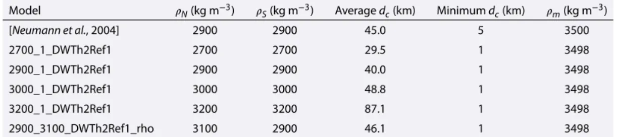
We adopt the bulk composition model of Wänke and Dreibus [1994] and distribute the radiogenic elements between the mantle and crust. Though the thickness of the crust does not change with time in our model, its thickness does vary laterally. Most of the models presented here use the crustal thickness model of Neumann et al. [2004] and a distribution of heat production between mantle and crust compatible with the average surface value inferred from orbital gamma ray measurements [Taylor et al., 2006; Hahn et al., 2011]. The crustal thickness model of Neumann et al. [2004] assumes a uniform crustal density of 2900 kg m−3_,

but a variety of crustal thickness models have been proposed that use a broader range of bulk crustal den-sities between 2700 and 3100 kg m−3_{[Wieczorek and Zuber, 2004] where the higher values are supported}

by petrological constraints obtained from major element analysis of Martian meteorites and surface rocks

(7)

Table 3. Crustal Thickness Models Used in Our Simulationsa Model _𝜌_N(kg m−3₎ _𝜌 S(kg m−3) Averagedc(km) Minimumdc(km) 𝜌m(kg m−3) [Neumann et al., 2004] 2900 2900 45.0 5 3500 2700_1_DWTh2Ref1 2700 2700 29.5 1 3498 2900_1_DWTh2Ref1 2900 2900 40.0 1 3498 3000_1_DWTh2Ref1 3000 3000 48.8 1 3498 3200_1_DWTh2Ref1 3200 3200 87.1 1 3498 2900_3100_DWTh2Ref1_rho 3100 2900 46.1 1 3498 a_𝜌

Nand𝜌Sare the densities of the northern lowlands and southern highlands, respectively; averagedcis the average crustal thickness of the model; minimumd_cis the minimum crustal thickness of the model; and𝜌_mis the upper mantle density.

[Baratoux et al., 2014]. Moreover, a dichotomy in crustal density rather than crustal thickness may as well be compatible with the constraints from gravity and topography [Pauer and Breuer, 2008; Belleguic et al., 2005]. To test the sensitivity of our numerical simulations on the assumed crustal thickness model, we have con-structed a suite of crustal models with parameters that differ from those employed by Neumann et al. [2004]. These models follow closely the methodology described in Baratoux et al. [2014], with a few exceptions. First, we used a mantle density profile for the mantle that is consistent with the model of Wänke and Dreibus [1994]. The gravitational contribution from flattened interfaces in the mantle and core were accounted for by assuming that they were in hydrostatic equilibrium by requiring them to follow an equipotential surface con-sistent with the observed gravity field. We used crustal densities of 2700, 2900, 3000, and 3200 kg m−3_and

varied the average crustal thickness until a minimum value of 1 km was achieved, which always coincided with the center of the Isidis impact basin (see Table 3). For one model, we also accounted for a possible dif-ference in crustal densities north and south of the dichotomy boundary. For this model, we used a density of 2900 kg m−3_{for the southern highlands, 3100 kg m}−3_{for the northern lowlands, the dichotomy}

bound-ary as mapped by Andrews-Hanna et al. [2008], and the approach for calculating the gravity ﬁeld from lateral variations in crustal density as described in Wieczorek et al. [2013].

Since the thickness of the Martian crust shows signiﬁcant variations (between 5 and 100 km according to the model of Neumann et al. [2004], while its concentration in heat producing elements such as thorium varies only between 0.2 and 1 ppm [Taylor et al., 2006], crustal thickness variations have a greater impact on the surface heat ﬂux variability than variations in the distribution of heat-producing elements within the crust [Hahn et al., 2011]. Therefore, we neglect spatial variations in the abundance of the heat-producing elements and use instead an average value of 49 pW kg−1_{similar to the one obtained from gamma ray measurements}

[Taylor et al., 2006; Hahn et al., 2011]. The assumption that the surface composition reﬂects the entire under-lying crust will be discussed in section 4. Figure 1 shows the crustal thickness model of Neumann et al. [2004] and the associated crustal heat ﬂux produced only by the amount of radiogenic elements located in the crust (the heat production in the entire crust volume divided by the surface area). The thermal conductivity of the crust is varied between 2 and 3 W m−1_K−1_{[Clauser and Huenges, 1995; Seipold, 1998], while for the mantle a}

value of 4 W m−1_K−1_{is assumed [Hofmeister, 1999].}

2.3. Elastic Lithosphere Thickness Model

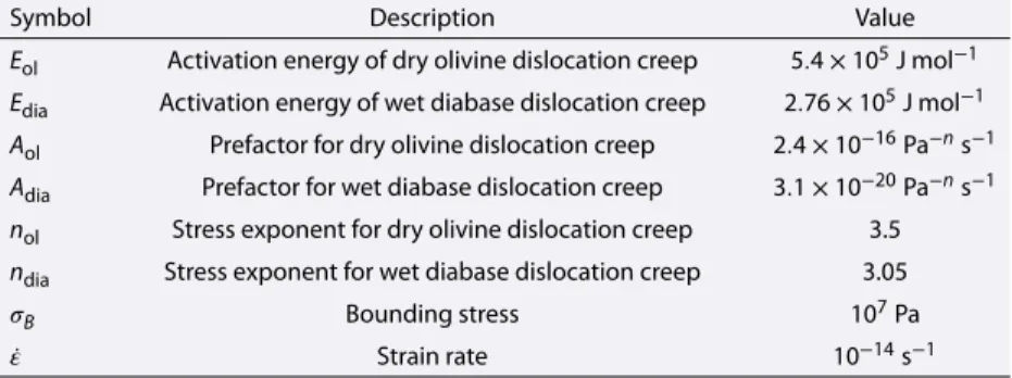
In most models we consider latitudinal variations of the mean annual surface temperature [Ohring and Mariano, 1968; Kieffer, 2013]. Although such surface temperature variations are insignificant for the convec-tion model, they may affect the mechanical thickness of the lithosphere, which we calculate employing a strength envelope formalism [McNutt, 1984] for the two-layer system consisting of crust and mantle. Given the long wavelengths and associated small curvatures considered here, we approximate the elastic thickness by the mechanical thickness of the lithosphere, i.e., the depth corresponding to the temperature at which the lithosphere loses its mechanical strength due to ductile flow [e.g., Grott and Breuer, 2008]. Following Burov and Diament [1995] and Grott and Breuer [2010], we assume a bounding stress of𝜎_B=10 MPa to define the base of the mechanical lithosphere:

Te= E R [ log( 𝜎 n BA ̇𝜀 )]−1 (6)

(8)

Table 4. Parameters Used for the Calculation of the Elastic Lithosphere Thickness

E_ol Activation energy of dry olivine dislocation creep 5.4 × 105_{J mol}−1

E_dia Activation energy of wet diabase dislocation creep 2_{.76 × 10}5_{J mol}−1

A_ol Prefactor for dry olivine dislocation creep 2.4 × 10−16_Pa−n_s−1

A_dia Prefactor for wet diabase dislocation creep 3_{.1 × 10}−20_Pa−n_s−1

n_ol Stress exponent for dry olivine dislocation creep 3.5

n_dia Stress exponent for wet diabase dislocation creep 3.05

𝜎B Bounding stress 107Pa

̇𝜀 Strain rate 10−14_s−1

where E, A, and n are rheological parameters; R is the gas constant;𝜎Bis a bounding stress, and ̇𝜀 is the strain

rate (Table 4). Note that the mechanical and elastic thickness will be similar for small curvatures and bending moments as appropriate for the geological features considered here, and from now we will simply use the term “elastic thickness.”

If the thicknesses D_e,cand D_e,mof the elastic cores of crust and mantle, respectively, are separated by a decou-pling layer of incompetent crust, the eﬀective elastic thickness of the system is signiﬁcantly reduced and can be calculated as [Burov and Diament, 1995]:

De= ( D3_e,m+ D3_e,c) 1 3 (7) Decoupling takes place in regions where the crustal thickness is particularly large and/or the lower crustal temperature is high, and we will show later that although present only in limited areas, crust-lithosphere decoupling is not uncommon for the present-day Mars. On the other hand, in the absence of an incompetent crustal layer, Deequals the sum of the two components, which act as a single plate. To compare our results

with the reported present-day elastic thickness value that is higher than 300 km at the north pole and higher than 110 km at the south pole, we use a strain rate of 10−14_s−1_{[Phillips et al., 2008] appropriate for deformation}

acting on the time scales of Martian obliquity variations [McGovern et al., 2004], which are believed to drive polar cap deposition [Phillips et al., 2008]. Note that a higher strain rate (i.e., of about 10−17_s−1_{) associated with}

deformation appropriate for mantle convection timescales is more appropriate to compute the elastic thick-ness values in volcanic regions like Tharsis and Elysium. Values computed for ̇𝜀 = 10−17_s−1_{are listed for each}

case presented in this study in the data sets of the supporting information.

3. Results

The parameters used in all simulations are listed in Tables 1–4. In Table 6 we provide output quantities for all the models discussed in this study. In addition to the present-day surface heat flux, elastic lithosphere thickness, CMB temperature, and CMB heat flux, we list the thermal Rayleigh numbers at the beginning and end of thermal evolution for each simulation. The initial Rayleigh number has been calculated by taking into account the average viscosity at 50 km depth (i.e., at the base of the initial upper thermal boundary layer). This value depends on the initial parameters (i.e., initial temperature, reference viscosity, depth dependence of the viscosity, and thermal expansion coefficient). Note that the Ra changes during the thermal evolution. The final Rayleigh number shown in column 10 of Table 6 has been calculated based on the average viscosity at the base of the stagnant lid after 4.5 Gyr of thermal evolution. Typically, the difference between the initial and final Rayleigh numbers is of about 1–2 orders of magnitude for cases employing the crustal thickness model of Neumann et al. [2004] and a depth-dependent viscosity. For case 8, where no depth dependence of the viscosity has been used, the initial and final Rayleigh numbers are similar. However, during the evolution, Ra first increases due to an initial stage of mantle heating caused by the radioactive elements (the amplitude and duration of mantle heating depend, however, on the initial temperature and reference viscosity) and then decreases due to mantle cooling. Hence, although the initial and final Rayleigh numbers for case 8 are similar, the convection vigor is higher during the evolution but decreases with time, and in this particular case it is close to the starting value. For cases employing a large crustal thickness (cases 26–32), the difference between the initial and final Rayleigh numbers is of about 3–4 orders of magnitude. This is due to the lower amount of radiogenic elements present in the mantle and hence a more efficient mantle cooling.

(9)

Figure 2. Laterally averaged viscosity proﬁles assuming a moderate activation volumeV = 6cm3_mol−1_{(dashed line;}

case 1 in Tables 5 and 6), an additional viscosity jump of 50 in the midmantle (dashed-dotted line; case 2), and a large activation volumeV = 10cm3mol−1_{(solid line; case 3).}

3.1. Lateral Variations of the Surface Heat Flux In our models we consider three end-member cases for the depth dependence of the viscosity and use either a moderate or a strong increase of vis-cosity with depth or additionally a visvis-cosity jump in the midmantle. In Figure 2, we show laterally averaged viscosity proﬁles obtained after 4.5Gyr of evolution that correspond to these three cases (labeled as cases 1–3 in Table 6) using a con-stant thermal expansivity value of 2.5×10−5_K−1_{. In}

Figures 3a–3c we show the present-day total sur-face heat flux, while in Figures 3d–3f ) we show the difference between the total heat flux and the heat flux produced by the crustal radiogenic elements (Figure 1b). The resulting heat flux shows the man-tle contribution, which includes the crustal heat flux due to secular cooling. However, the latter contribu-tion is minor. The three maps are obtained using an activation volume V = 6 cm3_mol−1_{(Figures 3a and 3d), including an additional viscosity jump of a factor of 50}

in the midmantle (Figures 3b and 3e) or using an activation volume of 10 cm3_mol−1_{(Figures 3c and 3f ). We also}

considered a case with no depth dependence of the viscosity (case 8 in Table 6); i.e., V = 0 cm3_mol−1_{. However,}

no significant differences in the heat flux maps are observed when using V = 0 cm3_mol−1_{and V = 6 cm}3_mol−1_.

The surface heat flux pattern is dominated by the crustal structure, which leads to similar distributions for all three models of Figure 3, with a larger heat flux in the southern highlands and a smaller heat flux in the northern lowlands. Although the average surface value for these three models varies only between 23.6 and 23.9 mW m−2_{, the convection pattern and the mantle heat flux distribution can vary significantly depending}

Figure 3. (a–c) Total surface heat ﬂux variations and (d–f ) the corresponding mantle contribution for the three diﬀerent viscosity models in Figure 1. Figure 3a using an activation volumeV = 6cm3_mol−1_{(case 1 in Tables 5 and 6), Figure 3b considering an additional viscosity jump of 50 in the midmantle (case 2),}

and Figure 3c assuming an activation volumeV = 10cm3_mol−1_{(case 3). Figures 3d–3f show the corresponding mantle heat ﬂux obtained by subtracting}

the contribution of the crustal heat producing elements from the total surface heat flux in Figures 3a–3c. Note that the mantle heat flux includes the secular cooling contribution of the crustal heat flux.

(10)

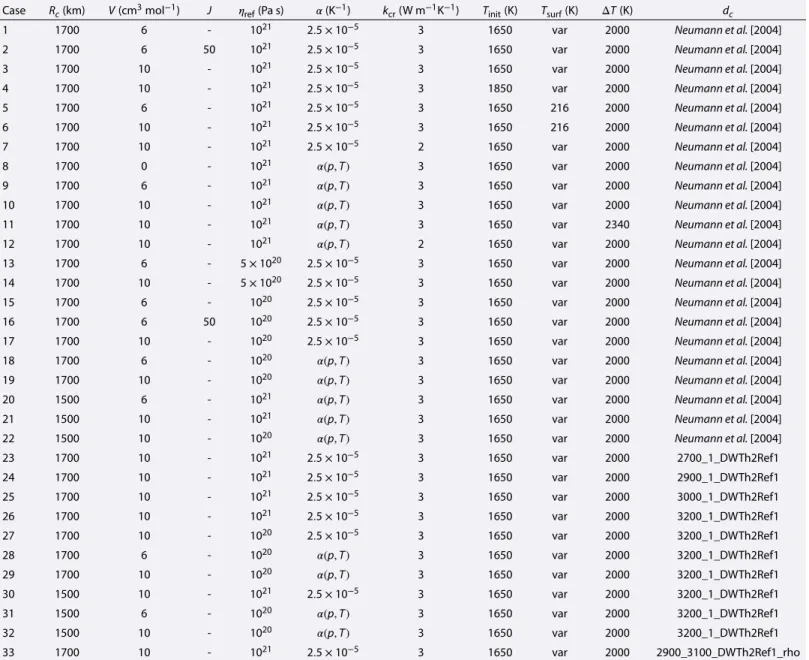
Table 5. Input Parameters for All Simulations Discussed in the Texta Case R_c(km) V(cm3_mol−1₎ _J _𝜂

ref(Pa s) 𝛼(K−1) kcr(W m−1K−1) Tinit(K) Tsurf(K) ΔT(K) dc

1 1700 6 - 1021 2.5 × 10−5 ₃ ₁₆₅₀ _var ₂₀₀₀ _{Neumann et al. [2004]}

2 1700 6 50 1021 ₂_{.5 × 10}−5 ₃ ₁₆₅₀ _var ₂₀₀₀ _{Neumann et al. [2004]}

3 1700 10 - 1021 2.5 × 10−5 3 1650 var 2000 Neumann et al. [2004]

4 1700 10 - 1021 ₂_{.5 × 10}−5 ₃ ₁₈₅₀ _var ₂₀₀₀ _{Neumann et al. [2004]}

5 1700 6 - 1021 ₂_{.5 × 10}−5 ₃ ₁₆₅₀ ₂₁₆ ₂₀₀₀ _{Neumann et al. [2004]}

6 1700 10 - 1021 2.5 × 10−5 ₃ ₁₆₅₀ ₂₁₆ ₂₀₀₀ _{Neumann et al. [2004]}

7 1700 10 - 1021 ₂_{.5 × 10}−5 ₂ ₁₆₅₀ _var ₂₀₀₀ _{Neumann et al. [2004]}

8 1700 0 - 1021 𝛼(p, T) 3 1650 var 2000 Neumann et al. [2004]

9 1700 6 - 1021 _{𝛼(p, T)} ₃ ₁₆₅₀ _var ₂₀₀₀ _{Neumann et al. [2004]}

11 1700 10 - 1021 _{𝛼(p, T)} ₃ ₁₆₅₀ _var ₂₃₄₀ _{Neumann et al. [2004]}

12 1700 10 - 1021 _{𝛼(p, T)} ₂ ₁₆₅₀ _var ₂₀₀₀ _{Neumann et al. [2004]}

13 1700 6 - 5 × 1020 2.5 × 10−5 ₃ ₁₆₅₀ _var ₂₀₀₀ _{Neumann et al. [2004]}

14 1700 10 - 5 × 1020 ₂_{.5 × 10}−5 ₃ ₁₆₅₀ _var ₂₀₀₀ _{Neumann et al. [2004]}

15 1700 6 - 1020 2.5 × 10−5 ₃ ₁₆₅₀ _var ₂₀₀₀ _{Neumann et al. [2004]}

16 1700 6 50 1020 ₂_{.5 × 10}−5 ₃ ₁₆₅₀ _var ₂₀₀₀ _{Neumann et al. [2004]}

17 1700 10 - 1020 ₂_{.5 × 10}−5 ₃ ₁₆₅₀ _var ₂₀₀₀ _{Neumann et al. [2004]}

23 1700 10 - 1021 ₂_{.5 × 10}−5 ₃ ₁₆₅₀ _var ₂₀₀₀ _{2700_1_DWTh2Ref1} 24 1700 10 - 1021 ₂_{.5 × 10}−5 ₃ ₁₆₅₀ _var ₂₀₀₀ _{2900_1_DWTh2Ref1} 25 1700 10 - 1021 ₂_{.5 × 10}−5 ₃ ₁₆₅₀ _var ₂₀₀₀ _{3000_1_DWTh2Ref1} 26 1700 10 - 1021 ₂_{.5 × 10}−5 ₃ ₁₆₅₀ _var ₂₀₀₀ _{3200_1_DWTh2Ref1} 27 1700 10 - 1020 2.5 × 10−5 ₃ ₁₆₅₀ _var ₂₀₀₀ _{3200_1_DWTh2Ref1} 28 1700 6 - 1020 _{𝛼(p, T)} ₃ ₁₆₅₀ _var ₂₀₀₀ _{3200_1_DWTh2Ref1} 29 1700 10 - 1020 𝛼(p, T) 3 1650 var 2000 3200_1_DWTh2Ref1 30 1500 10 - 1021 ₂_{.5 × 10}−5 ₃ ₁₆₅₀ _var ₂₀₀₀ _{3200_1_DWTh2Ref1} 31 1500 6 - 1020 _{𝛼(p, T)} ₃ ₁₆₅₀ _var ₂₀₀₀ _{3200_1_DWTh2Ref1} 32 1500 10 - 1020 _{𝛼(p, T)} ₃ ₁₆₅₀ _var ₂₀₀₀ _{3200_1_DWTh2Ref1} 33 1700 10 - 1021 ₂_{.5 × 10}−5 ₃ ₁₆₅₀ _var ₂₀₀₀ _{2900_3100_DWTh2Ref1_rho} a_R

cis the core radius,Vis the activation volume,Jis an additional viscosity jump in the midmantle,𝜂refis the reference viscosity,𝛼is the thermal expansivity,

k_cris the crust thermal conductivity,T_initis the initial mantle temperature,T_surfis the surface temperature,ΔTis the temperature diﬀerence across the mantle, and

d_cis the crustal thickness model used (Table 3).

Table 6. Summary of Results for All Simulations Discussed in the Texta

Case F_s[min_{, max}] (mW m−2₎ _T

e[min, max] (km) FsInSight(mW m−2) TeNP(km) TeSP(km) TCMB(K) FCMB(mW m−2) Rainitial Raﬁnal

1 23.9[18.4,32.0] 226 [83,275] 21.4 262 219 2092.8 2.3 2.02e+07 3.04e+06 2 23.9[17.7,30.2] 227[101,284] 21.8 261 185 2141.3 2.0 2.02e+07 2.04e+06 3 23.6[17.3,31.0] 233 [97,287] 20.2 249 233 2141.3 1.6 4.07e+07 2.84e+05 4 24.7[18.2,32.6] 217 [81,275] 22.6 237 242 2154.6 2.1 4.45e+08 8.65e+05 5 24.1[18.7,32.7] 222 [84,262] 21.5 247 208 2102.3 2.6 2.06e+07 4.36e+06 6 23.9[17.3,32.4] 229 [86,294] 20.9 242 219 2158.6 2.2 4.15e+07 3.50e+05 7 23.7[16.4,34.4] 193 [44,311] 21.9 245 179 2129.0 1.8 4.07e+07 9.09e+04 8 23.7[18.8,30.2] 228[102,260] 21.3 255 226 2112.9 1.4 1.20e+07 6.46e+07

(11)

Table 6. (continued)

Case F_s[min, max] (mW m−2₎ _T

e[min, max] (km) FsInSight(mW m−2) TeNP(km) TeSP(km) TCMB(K) FCMB(mW m−2) Rainitial Raﬁnal

9 23.4[18.2,30.7] 234 [95,273] 20.8 263 230 2150.4 2.0 3.44e+07 3.48e+06 10 23.2[17.6,30.6] 239[100,294] 20.6 267 228 2181.9 1.4 6.93e+07 3.84e+05 11 24.5[18.6,33.9] 218 [75,267] 21.6 251 222 2247.1 3.5 8.34e+07 2.05e+06 12 23.3[17.0,32.5] 198 [48,287] 20.1 257 170 2174.2 1.5 6.93e+07 2.84e+05 13 24.1[18.5,32.5] 223 [81,269] 21.5 254 219 2056.8 2.7 4.03e+07 2.74e+06 14 23.8[17.4,36.1] 230 [66,293] 21.9 269 219 2109.6 2.1 8.13e+07 4.88e+05 15 25.7[19.3,51.3] 203 [42,262] 23.5 243 190 1954.9 3.6 2.02e+08 3.20e+07 16 24.7[17.4,36.8] 219 [65,298] 21.0 197 233 2031.2 3.0 2.02e+08 6.35e+06 17 24.2[17.2,49.9] 228 [44,307] 20.3 256 253 2034.7 2.8 4.07e+08 6.95e+06 18 24.1[18.9,31.3] 224 [94,266] 21.4 257 230 2032.9 3.4 3.44e+08 6.44e+06 19 24.2[17.6,39.3] 226 [60,294] 21.5 269 203 2071.0 3.0 6.93e+08 1.52e+06 20 26.1[20.3,34.9] 205 [74,245] 23.2 238 203 2229.0 1.5 4.76e+07 1.31e+07 21 26.0[19.4,34.7] 208 [74,258] 23.0 240 205 2236.3 0.6 9.63e+07 2.23e+06 22 26.8[19.7,44.6] 200 [50,260] 23.1 240 211 2128.6 2.4 9.63e+08 4.18e+06 23 24.0[20.1,30.9] 207[149,251] 21.2 238 224 2176.1 1.8 4.07e+07 1.44e+06 24 23.6[18.1,31.1] 225 [97,280] 21.2 264 222 2150.3 1.7 4.07e+07 5.97e+05 25 23.3[16.2,35.3] 241 [68,323] 19.0 289 210 2128.3 1.6 4.07e+07 2.01e+05 26 23.9[10.7,38.5] 319 [61,547] 18.8 494 91 2031.7 2.2 4.07e+07 8.86e+03 27 24.4[10.6,40.1] 307 [58,563] 19.3 505 88 1970.0 2.8 4.07e+08 2.69e+04 28 24.7[12.1,36.0] 271 [66,469] 20.0 426 88 1894.1 3.7 3.46e+08 8.83e+03 29 24.3[10.9,37.7] 298 [63,540] 19.5 478 93 1978.4 2.9 6.98e+08 1.35e+05 30 26.4[11.9,42.6] 266 [55,496] 20.9 444 78 2058.6 1.0 5.65e+07 7.74e+04 31 27.3[13.5,38.7] 220 [62,409] 22.3 369 77 1953.9 2.7 4.76e+08 7.48e+04 32 27.1[12.4,41.0] 240 [58,474] 21.8 422 78 2025.4 2.1 9.63e+08 4.50e+05 33 23.4[17.1,37.8] 237 [62,300] 24.2 264 212 2137.3 1.5 4.07e+07 4.12e+05

a_{All values in columns 2–8 refer to the present day.}_F

s[min, max], average surface heat ﬂux with minimum and maximum values;Te[min, max], average elastic thickness with minimum and maximum values calculated assuming a strain rate ̇𝜀 = 10−14_s−1_;_F

sInSight, surface heat ﬂux at InSight location;TeNP, elastic litho-sphere thickness averaged below the north pole ice cap (i.e., within 10∘from the north pole);T_eSP_{, elastic lithosphere thickness averaged below the south pole}

ice cap (i.e., within 5∘from the south pole);T_CMB, core-mantle boundary temperature; andF_CMB, core-mantle boundary heat ﬂux. Column 9 shows the initial ther-mal Rayleigh number calculated at a depth of 50 km below the surface (i.e., at the base of the initial therther-mal boundary layer). Column 10 shows the ﬁnal therther-mal Rayleigh number (i.e., after 4.5 Gyr of evolution) calculated at the bottom of the stagnant lid.

on the viscosity structure. For a viscosity increase of more than 2 orders of magnitude with depth, the signature of mantle plumes becomes clearly visible in both the mantle heat ﬂux (Figure 3f ) and in the total surface heat ﬂux (Figure 3c). In the three cases shown in Figure 3, lateral anomalies in the mantle introduced by plumes range from 2.2 mW m−2_{for case 1 (V = 6 cm}3_mol−1_{) to 5.4 mW m}−2_{for case 3 (V = 10 cm}3_mol−1_{) relative to}

the average value of around 17 mW m−2_.

The coefficient of thermal expansion𝛼 increases with temperature but decreases with depth and directly impacts the buoyancy forces. At the CMB the pressure dependence of𝛼 dominates and the temperature gra-dient is reduced due to inefficient heat transport associated with decreased buoyancy. A small temperature gradient at the CMB reduces the excess temperature of mantle plumes, and although the surface heat flux remains unaffected on average, its lateral variations are reduced for cases accounting for a temperature- and pressure-dependent thermal expansivity compared to cases assuming a constant value of𝛼 of 2.5 × 10−5_K−1

(compare Figures 3c and 4a, and case 1 and 9, 3 and 10, 7 and 12, 15 and 18, and 17 and 19 in Table 6). The reference viscosity impacts the cooling eﬃciency of the mantle, resulting in a cooler interior for a reference viscosity of 1020_{Pa s compared to a reference viscosity of 10}21_{Pa s. An eﬃcient cooling of the mantle also}

maintains a higher-temperature gradient across the CMB. This in turn aﬀects the excess temperature of mantle plumes resulting in temperature diﬀerences between hot upwellings and ambient mantle of up to 85 K for a reference viscosity of 1020_{Pa s, which is about 1.5 times higher than for a reference viscosity of 10}21_{Pa s.}

(12)

Figure 4. (a, b) Total surface heat ﬂux variations and (c, d) the corresponding mantle contribution for a temperature-and depth-dependent thermal expansivity, an activation volumeV = 10cm3mol−1_{, and two diﬀerent reference}

viscosities. Figure 4a using a reference viscosity of1021Pa s (case 10 in Tables 5 and 6) and Figure 4b considering a reference viscosity of1020Pa s (case 19).

The presence of stronger mantle thermal anomalies in the low reference viscosity case may produce local surface heat ﬂux values of up to 50 mW m−2_{. Here heat ﬂux anomalies introduced by mantle plumes reach}

values as high as 23.6 mW m−2_{relative to an average mantle value of 17.9 mW m}−2_{(case 17 in Table 6). Figure 4}

shows the eﬀect for two cases considering a temperature- and pressure-dependent thermal expansivity and reference viscosities of 1021_{Pa s (Figure 4a) and 10}20_{Pa s (Figure 4b). Nevertheless, high heat ﬂux values}

remain conﬁned to limited regions and the average surface heat ﬂux lies around 24.5 mW m−2_{for all cases}

that considered a core size of 1700 km, regardless of the viscosity model, thermal expansivity, crustal thickness models or crustal thermal conductivity (Table 6).

We also varied the size of the core by running models with core radii of 1700 and 1500 km for which we con-sider two exothermic and two exothermic and one endothermic phase transitions, respectively. Comparing cases 9, 10, 19, 26, 28, and 29 (all with a core size of 1700 km) with cases 20, 21, 22, 30, 31, and 32 (all with a core size of 1500 km) in Table 6 we obtain an average surface heat ﬂux between 23.2 and 24.7 mW m−2_{for the}

1700 km core size compared to 26–27.3 mW m−2_{for the smaller core size. When the core size is smaller, the}

total abundances of radiogenic elements in the silicate part of the planet is higher, accounting for the higher heat ﬂuxes. For the case of the smaller core size the surface heat ﬂux is 2–3 mW m−2_{higher compared to the}

simulations with a larger core.

Most of the cases considered here employ the crustal thickness model of Neumann et al. [2004]. However, to assess the robustness of our results, we also test a variety of crustal thickness models that consider different crustal densities and average crustal thicknesses (cases 23 to 33 in Table 6). The surface average heat flux and the heat flux at the InSight location are similar to the values obtained when using the model of Neumann et al. [2004]. For the north pole elastic thickness, we obtain values that increase from 240 to 500 km as the crustal density increases from 2700 to 3200 kg m−3_{(cf. cases 23–26 in Table 6). Moreover, the highest heat}

ﬂux variations of more than 30 mW m−2_{are observed when using a crustal density of 3200 kg m}−3_{, for which}

crustal thickness variations exceed 200 km. In this case, the crust contains most of the heat sources, and hence, large variations in crustal thickness cause signiﬁcant peak-to peak variations of the surface heat ﬂux.

(13)

Figure 5. (a–c) Total surface heat ﬂux variations and (d–f ) the corresponding mantle contribution assuming an activation volumeV = 10cm3mol−1_{and three}

diﬀerent crustal thickness models. Figure 5a uses a crustal density of 3100 kg m−3_{for the northern lowlands and 2900 kg m}−3_{for the southern highlands and a}

mean crustal thickness of 46.1 km (case 33 in Tables 5 and 6), Figure 5b using the crustal thickness model of Neumann et al. [2004] which has a mean crustal thickness of 45 km (case 3), and Figure 5c using a crustal density of 3200 kg m−3_{that results in a mean crustal thickness of 87.1 km (case 26).}

In Figure 5 we show the surface heat ﬂux variations (a–c) and the mantle contribution (d–f ) for three diﬀerent crustal models: a model with a mean crustal thickness of 46.1 km that uses a crustal density of 3100 kg m−3

north of the dichotomy boundary and 2900 kg m−3_{south of the boundary (Figures 5a and 5c and case 33 in}

Table 6), a model using the crustal thickness model of Neumann et al. [2004] which has a mean crustal thickness of 45 km (Figures 5b and 5e and case 3), and a model employing a uniform crustal density of 3200 kg m−3

Figure 6. Equal-area crustal thickness histograms using a bin size of 2 km for a model considering a crustal density of 3100 kg m−3

north of the dichotomy boundary and 2900 kg m−3_{south of}

the boundary (model 2900_3100_DWTh2Ref1_rho in Table 3 and case 33 in Tables 5 and 6), the crustal thickness from

Neumann et al. [2004] (case 3 in Tables 5 and 6), and a model

that uses a uniform crustal density of 3200 kg m−3_(model

3200_1_DWTh2Ref1 in Table 3 and case 26 in Tables 5 and 6).

resulting in a mean crustal thickness of 87.1 km (Figures 5c and 5f and case 26). While Figures 5b and 5c show a dichotomy in the sur-face heat flux that follows the crustal thickness dichotomy, Figure 5a shows a rather uniform surface heat flux distribution, apart from the Tharsis region. Of the three models in this figure, the model in Figures 5c and 5f exhibits the highest surface heat flux variations, which is a result of this model possessing the largest lateral variations in crustal thickness. Figure 6 shows equal-area histograms of crustal thick-ness for the three models in Figure 5. While the models assuming a uniform crustal den-sity show a bimodal distribution of the crustal thickness with peaks at 30 and 60 km for the model of Neumann et al. [2004], and at 60 and 115 km for the model assuming a uniform density of 3200 kg m−3_{, the model employing}

a dichotomy in crustal density shows a more broad distribution with a major peak at 50 km.

(14)

Figure 7. (a) Comparison of the average surface heat ﬂux and the heat ﬂux at the InSight location. The blue shaded regions show the simulations which use a core radius of 1500 km, the yellow shaded region shows the cases employing a crustal density higher or equal 3000 kg m−3_{, and the red shaded region shows}

the case using a crustal thickness model, which assumes different densities for the northern lowlands and the southern highlands; (b) the difference between the surface heat flux and the heat flux at the InSight location. The colors are the same as in Figure 7a. The case numbers correspond to the case numbers listed in Table 6.

Other parameters such as the initial mantle temperature, the crustal conductivity, and the surface temperature play a secondary role for the surface heat ﬂux, but they may aﬀect the magnitude and the distribution of the elastic thickness (Table 6).

3.2. Heat Flux at InSight Location

In our models, no mantle plume is present beneath the InSight landing site located at a distance of about 1480 km from the Elysium volcanic center. Even if an upwelling is located below the Elysium volcanic con-struct, the induced heat flux anomaly remains confined within a radius of 815 km from the plume center. For all the cases investigated here, independent of the presence of a mantle upwelling at Elysium, the surface heat flux at the InSight location lies between 18.8 and 24.2 mW m−2_{, close to the surface average which varies}

between 23.2 and 27.3 mW m−2_.

In Figure 7 we show the average surface heat flux and the heat flux at the InSight location for all simulations listed in Table 6 as well as the difference between the two values. The average surface heat flux and the heat flux at InSight location is up to 3 mW m−2_{higher for models assuming a core radius of 1500 km compared to}

models with a core radius of 1700 km (blue shaded region in Figure 7a). However, regardless of the core size, the difference between the average surface heat flux and the heat flux at the InSight location lies between 2 and 3 mW m−2_{for most models employing a crustal density lower than 3000 kg m}−3_{(cases 1–24 in Table 6}

and in Figure 7b). Simulations using a crustal density higher than 3000 kg m−3_{show a diﬀerence of about}

5 mW m−2_{between the average surface heat ﬂux and the heat ﬂux at the InSight location (yellow shaded}

region in Figure 7b and cases 25–32 in Table 6), since in these cases the crustal thickness dichotomy leads to a more pronounced dichotomy in the surface heat flux. If, however, a difference in crustal density between the northern lowlands and the southern highlands is assumed, the resulting smaller variations in the crustal thickness lead to a difference smaller than 1 mW m−2_{between the heat flux at the InSight location and the}

average surface heat ﬂux (red shaded region in Figure 7b).

The smallest heat ﬂux values at the InSight location are obtained for cases employing a crustal density of 3200 kg m−3_{and hence an average crustal thickness of around 87.1 km (cases 26–32 in Table 6). In these}

cases, the value at the InSight landing site is up to 2 mW m−2_{lower than the value obtained using the model}

by Neumann et al. [2004]. Since most of the heat producing elements are located in the crust, variations of the surface heat ﬂux are mainly caused by crustal thickness variations and values as small as 10 mW m−2_are

obtained in regions of thin crust (i.e., Hellas basin), while values up to 38 mW m−2_{are obtained in the Tharsis}

area (Figure 6). The highest value at the InSight landing site is attained for the case using a diﬀerence in crustal density between the northern lowlands and southern highlands, which reduces the diﬀerence in thickness

(15)

Figure 8. (a) Total surface heat ﬂux variations and (b) elastic thickness variations for a reference viscosity of1021_{Pa s and an activation volume}_{V = 10}_cm3_mol−1

(case 3 in Tables 5 and 6).

across the dichotomy boundary when compared to the constant crustal density models. For this model, the InSight value is less than 1 mW m−2_{away from the average surface heat ﬂux (Figure 7).}

3.3. Elastic Lithosphere Thickness

We use the strength envelope formalism (cf. section 2.3) to compute the elastic lithospheric thickness and compare the obtained values with the present-day estimates at the north and south poles.

The crustal structure is the main agent that controls the elastic lithosphere thickness, and a layer of incom-petent crust can be found at present-day below regions of thick crust. Nevertheless, mantle upwelling and downwellings can locally cause thinning or thickening of the elastic lithosphere. In Figure 8 we show the surface heat ﬂux and the corresponding elastic thickness calculated using a strain rate ̇𝜀=10−14_s−1_{for a}

rep-resentative case (case 3 in Table 6) that assumes a strong depth dependence of viscosity in the mantle. The crustal structure directly affects the heat flux and elastic thickness distribution resulting in a dominant degree one pattern, with elevated heat flux and smaller elastic thickness in the southern hemisphere compared to the northern lowlands. The signal of mantle upwellings is superimposed on both the heat flux and elastic thickness degree one pattern induced by the crustal thickness variations.

Most cases are characterized by maximum values of the elastic lithosphere thickness well above 250 km and by lateral variations of more than 100 km. The highest values of the elastic thickness correlate with the lowest heat ﬂuxes that are reached in regions of thin crust (i.e., Hellas basin and regions close to the north pole in Accidalia Planitia and Utopia Planitia).

For models using a crustal density of 3200 km and hence a crustal thickness of up to 215 km, most of the radioactive elements are located in the crust while the mantle is considerably depleted. This is reflected also in the mantle and CMB temperatures which are lower than in cases using the crustal thickness model of Neumann et al. [2004]. Moreover, the mantle temperatures beneath the northern hemisphere are significantly lower than the ones beneath the southern part, since the latter is covered by a thicker crust that prevents efficient cooling of the interior. For such models, the elastic lithosphere thickness at the north pole exceeds 350 km. However, the values obtained at the south pole lie below 95 km.

Regions with the lowest elastic thickness are located in the Tharsis area where, depending on the model parameters, values as low as 42 km are obtained for ̇𝜀=10−14_s−1_{. Note that for} _̇𝜀=10−17_s−1_{the lowest value,}

which is obtained in the same region, is smaller by about 10 km. All values for the elastic lithosphere thickness computed with ̇𝜀 = 10−14_s−1_and _{̇𝜀 = 10}−17_s−1_{are listed in the data sets of the supporting information. Such}

small values are observed either for models with a reference viscosity lower than 1021_{Pa s and thus a thinner}

boundary layer or for models with a crust thermal conductivity of 2 W m−1_K−1_{, for which the lithospheric}

tem-peratures are higher because of the more eﬃcient thermal insulation compared to cases using 3 W m−1_K−1_.

Furthermore, in most of our models a mechanically incompetent layer is present today around Arsia Mons and results in small elastic thickness values in that region due to the decoupling of crust and lithosphere.

(16)

4. Discussion and Conclusions

We have investigated the effects of mantle parameters on the present-day spatial variations of the Martian surface heat flux. Using fully dynamical 3-D mantle convection models, we have tested the influence of the reference viscosity, viscosity variations with depth, initial mantle temperature, surface temperature, temperature- and pressure-dependent thermal expansivity, crust conductivity, core radius, and crustal thick-ness on the surface heat flux variations.

The results show that the average surface heat ﬂux varies between 23.2 and 27.3 mW m−2_{for all our models,}

while the surface heat ﬂux at the InSight location lies between 18.8 and 24.2 mW m−2_{, and shows a good}

correlation with the average value. For models assuming a smaller core radius of 1500 km, the average surface heat ﬂux is up to 3 mW m−2_{higher compared to models with a core radius of 1700 km.}

Depending on the assumed parameters, the maximum values of the surface heat ﬂux measured at the center of mantle plumes can reach 50 mW m−2_{. However, such high values remain conﬁned to limited surface regions}

with a radius smaller than about 815 km. The elastic lithosphere thickness varies laterally by more than 100 km and with peak-to peak diﬀerences as high as 244 km. If we use the crustal thickness model of Neumann et al. [2004], we obtain a present-day elastic thickness of around 270 km or lower at the north pole, around 30 km smaller than the value reported by Phillips et al. [2008], while at the south pole the values we obtain exceed 150 km and thus lie well above the minimum value of 110 km estimated for this region [Wieczorek, 2008]. Present-day elastic thickness values at the north pole could exceed 400 km if the crust is considerably thicker than in the model by [Neumann et al., 2004] (such as for our model with a crustal density of 3200 kg m−3_).

At the south pole the elastic thickness could lie below 95 km. This is explained by the fact that a thicker crust also contains a larger total abundance of radiogenic elements and is underlain by a mantle that is highly depleted. In this case, variations in the elastic lithosphere thickness and surface heat flux are mostly dominated by the spatial variations in crustal thickness. A difference between minimum and maximum crustal thickness of more than 200 km results in crustal heat flux variations larger than 30 mW m−2_{and, as a}

consequence, elastic thickness variations of more than 400 km. The lowest value of the present-day elastic thickness is attained in the vicinity of Arsia Mons and our models thus support previous studies that have proposed the presence of a local decoupling layer of incompetent crust to be responsible for the low-elastic thickness of this region [Grott and Breuer, 2010].

Even in the case in which a mantle plume develops at the Elysium site, its associated heat flux anomaly remains confined to within an 815 km radius. The InSight heat flux measurement, which will be taken approximately 1480 km away from Elysium, will likely remain undisturbed by the presence of a potential plume under-neath the volcanic center. Moreover, a mantle upwelling focused underunder-neath Elysium will most likely prevent additional mantle plumes to remain stable close to this region. The landing site proximity not only to the dichotomy boundary but also to Elysium further reduces the possibility for the heat flux measurement to be affected by the presence of a mantle plume. In fact, due to the specific crustal structure of this region, such a mantle plume would need to develop below a location consisting of regions with both thin and thick crust. In our models, the largest uncertainty in the average surface heat flux is due to the uncertainty in the radius of the Martian core. A small core radius of only 1500 km results in an average surface heat flux that is about 3 mW m−2_{higher than for a 1700 km core radius. The amplitude of the surface heat flux variations, however,}

remains similar, independent of the chosen core size. A thick crust (models 25–32 in Table 6) leads to a dif-ference of about 5 mW m−2_{between the average surface heat ﬂux and the value obtained at the InSight}

location. This value is about 2 mW m−2_{higher than the diﬀerence obtained for simulations which use the}

crustal thickness model of Neumann et al. [2004]. It is important to emphasize that the InSight mission will carry a seismometer to the surface of Mars and attempt to constrain the crustal structure and the size of the Martian core [Mimoun et al., 2012] and will help reduce the uncertainty in the average surface heat ﬂux in our simulations.

We have assumed that the abundance of radiogenic elements in the crust is uniform. Although the surface distribution of Th and K obtained from gamma ray measurements shows little variation in surface abun-dances, the gamma ray spectrometer (GRS) instrument can only map the composition of the upper few tens of centimeters of the Martian surface [Taylor et al., 2006]. The abundance of heat-producing elements with depth in the crust is unconstrained by these measurements, and it is plausible that the composition at depth might not reﬂect that of the surface. Although it has been argued that the crust has been built by both lava