HAL Id: hal-00317229
https://hal.archives-ouvertes.fr/hal-00317229
Submitted on 1 Jan 2004
HAL is a multi-disciplinary open access
archive for the deposit and dissemination of
sci-entific research documents, whether they are
pub-lished or not. The documents may come from
teaching and research institutions in France or
abroad, or from public or private research centers.
L’archive ouverte pluridisciplinaire HAL, est
destinée au dépôt et à la diffusion de documents
scientifiques de niveau recherche, publiés ou non,
émanant des établissements d’enseignement et de
recherche français ou étrangers, des laboratoires
publics ou privés.
AE-C data and CTIP modelling
H. Rishbeth, R. A. Heelis, I. C. F. Müller-Wodarg
To cite this version:
H. Rishbeth, R. A. Heelis, I. C. F. Müller-Wodarg. Variations of thermospheric composition according
to AE-C data and CTIP modelling. Annales Geophysicae, European Geosciences Union, 2004, 22 (2),
pp.441-452. �hal-00317229�
Annales Geophysicae (2004) 22: 441–452 © European Geosciences Union 2004
Annales
Geophysicae
Variations of thermospheric composition according to AE-C data
and CTIP modelling
H. Rishbeth1, R. A. Heelis2, and I. C. F. M ¨uller-Wodarg3,4
1School of Physics and Astronomy, University of Southampton, Southampton SO17 1BJ, UK
2William B. Hanson Center for Space Sciences, The University of Texas at Dallas, P. O. Box 830688, Richardson, Texas
75083-0588, USA
3Atmospheric Physics Laboratory, University College London, 67-73 Riding House Street, London W1W 7EJ, UK 4now at: Space and Atmospheric Lab, Imperial College London, Prince Consort Road, London SW7 2BW, UK
Received: 12 February 2003 – Revised: 16 June 2003 – Accepted: 18 June 2003 – Published: 1 January 2004
Abstract. Data from the Atmospheric Explorer C satellite,
taken at middle and low latitudes in 1975–1978, are used to study latitudinal and month-by-month variations of ther-mospheric composition. The parameter used is the “com-positional P -parameter”, related to the neutral atomic oxy-gen/molecular nitrogen concentration ratio. The midlatitude data show strong winter maxima of the atomic/molecular ra-tio, which account for the “seasonal anomaly” of the iono-spheric F2-layer. When the AE-C data are compared with the empirical MSIS model and the computational CTIP ionosphere-thermosphere model, broadly similar features are found, but the AE-C data give a more molecular thermo-sphere than do the models, especially CTIP. In particular, CTIP badly overestimates the winter/summer change of com-position, more so in the south than in the north. The semi-annual variations at the equator and in southern latitudes, shown by CTIP and MSIS, appear more weakly in the AE-C data. Magnetic activity produces a more molecular thermo-sphere at high latitudes, and at mid-latitudes in summer.
Key words. Atmospheric composition and structure
(ther-mosphere – composition and chemistry)
1 Introduction
The seasonal anomaly in the ionospheric F2-layer was re-ported by Berkner et al. (1936) and has been extensively studied, for example, by Yonezawa (1971) and Torr and Torr (1973). Its main feature is that the peak electron density
NmF2 is greater in winter than in summer, most noticeably
in high mid-latitudes in the North American/European and Australasian sectors at solar maximum. However, in other longitudes, and more generally in lower latitudes, the pre-dominant variation of NmF2 is more or less semiannual, with maxima at or soon after the equinoxes. This paper is mainly concerned with the seasonal changes in neutral composition
Correspondence to: I. C. F. M¨uller-Wodarg
(i.mueller-wodarg@imperial.ac.uk)
of the thermosphere that largely determine this behaviour of
NmF2.
According to the generally accepted theory, NmF2 de-pends on the atomic/molecular ratio (in particular, the O/N2
ratio) of the ambient neutral air, and, of course, on the flux of solar ionizing radiation. Rishbeth and Setty (1961) suggested that the seasonal anomaly is caused by changes in the atomic/molecular ratio in the neutral thermosphere at F2-layer heights. Duncan (1969) suggested that these composition changes are caused by a global summer-to-winter circulation in the thermosphere, with the atomic oxy-gen/molecular nitrogen (O/N2) ratio being decreased by
up-welling of air in the tropics and summer mid-latitudes, and greatly enhanced in zones of downwelling that lie just equatorward of the winter auroral ovals. The location of the auroral zones, of course, depends on geomagnetic co-ordinates and, as a (rather complicated) consequence, the (O/N2) ratio and NmF2 vary annually in some longitude
sectors, semiannually in others. This was demonstrated in theoretical modelling by Millward et al. (1996a) and more comprehensively by Zou et al. (2000). The patterns of downwelling and upwelling were modelled by Rishbeth and M¨uller-Wodarg (1999). On the experimental side, the sea-sonal changes in the O/N2 ratio at mid-latitudes were
de-tected experimentally by von Zahn et al. (1973), using the ESRO 4 Gas Analyzer, and by Mauersberger et al. (1976), using the Open-Source Spectrometer on the Atmospheric Ex-plorer AE-C satellite launched in November 1973 (Dalgarno et al., 1973). In this paper, we use data from the AE-C Neu-tral Atmosphere Temperature Experiment (NATE) (Spencer et al., 1973) to investigate how the O/N2ratio varies with
sea-son, latitude and longitude. In particular, we look for Dun-can’s zones of enhanced O/N2ratio near the winter auroral
ovals. The AE-C data present a good opportunity to search for these zones, though, with its orbital inclination of 67◦, the satellite does not reach the equatorward edge of the auroral ovals in all longitudes.
In Sect. 2 we describe in outline the instruments, the satel-lite orbit, and how we treated the data. We also briefly recall
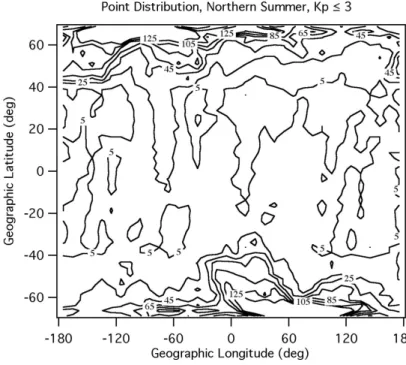
Fig. 1. Contour map showing number of data samples in AE-C composition data for northern summer, Kp≤3.
the main features of the Coupled Thermosphere-Ionosphere-Plasmasphere (CTIP) model (Fuller-Rowell et al., 1996, Millward et al., 1996b) as used by Rishbeth and M¨uller-Wodarg (1999) and Zou et al. (2000), and in the present pa-per for comparison with the AE-C data. We then present and discuss the composition data and model outputs in two ba-sic formats: plots versus latitude and longitude, for quiet and storm conditions (Sect. 3), and plots versus month and lon-gitude (Sect. 4); in both sections we first present the data, and then the CTIP results, and in Sect. 5 we compare these with values from the well-known MSIS-86 empirical model (Hedin, 1987). Section 6 discusses the results in more de-tail and Sect. 7 summarizes the main findings. Appendix A explains the “compositional P -parameter” that we use to present both the data and the model results.
2 Data, parameters and models
2.1 The NATE instrument on AE-C
The AE-C satellite was launched in November 1973 into an elliptical orbit with an inclination of 67.3◦with an apogee of 4000 km and a perigee between 160 km and 130 km. In April 1975 the orbit was circularized near 310 km and main-tained near this altitude until March 1977, when a circular orbit near 390 km was established. The orbit finally decayed in November 1978.
We use data from the Neutral Atmosphere Temperature Experiment, NATE (Spencer et al., 1973) operating at alti-tudes between 200 km and 450 km. Thus, the data are pre-dominantly collected from the circular orbit phases during 1975–1978. During this period, the monthly mean solar
10.7 cm flux was quite low, in the range of 70–100 units, and we have not divided the data according to solar flux. The NATE instrument was chosen to provide the largest continu-ous data set during that period. The spectrometer has a closed source in which the collected gases are in equilibrium with the chamber walls. The atomic oxygen is, therefore, detected as molecular oxygen, and the atomic oxygen concentration is derived by accounting for the factor of 2 in producing molec-ular oxygen and the ram pressure increase in the chamber produced by the supersonic motion of the spacecraft through the gas. The ambient molecular oxygen concentration can contribute up to 5% of the signal at the lowest altitudes con-sidered, so the atomic oxygen concentration may be slightly overestimated. The neutral composition is derived directly from the spectrometer outputs, while the neutral temperature is derived by examining the change in pressure as a baffle is scanned across the entrance aperture. The associated fit-ting procedure yields temperature data with reliability that depends upon conditions and delivers a data set that is less extensive than the composition data.
2.2 Treatment of the data
The data are recovered from unified abstract files that con-tain values for each pass averaged over a 15-s time interval or about 110 km along the satellite path. The data are thus spaced about 1◦in latitude at low and middle latitudes and about 1◦in longitude at the highest latitudes, with each 15-s 15-sample repre15-senting the average of about 4 point15-s. In thi15-s work we examine the global behaviour of the neutral com-position by collecting the data in cells of 2.5◦in latitude and 10◦in longitude. This bin size was chosen to provide a rea-sonable spatial resolution with a sensible sample size in most
H. Rishbeth et al.: Variations of thermospheric composition 443
Fig. 2. Contour plots for geographic latitudes 55◦N to 68◦N for Kp≤3, versus longitude and month. Above: Neutral O/N2concentration
ratio at heights 390 km (left), 280–400 km (right). Below: P -parameter at heights 390 km (left), 280–400 km (right).
bins. The AE-C satellite was not operated continuously, and the planned operations resulted in the majority of the data being taken at latitudes above 50◦in each hemisphere.
During this study we examine variations in composition as a function of latitude and longitude for a given season and as a function of longitude and season in a given latitude range. The number of data points is insufficient to examine global distributions separated by local time. However, by compar-ing the data obtained at 09:00–15:00 LT with that obtained for all local times, we found that the composition does not vary greatly from day to night (in line with theoretical re-sults, see Sect. 5), so we have combined data from all local times. Although separating the data by Kp produces some
gaps in the global distributions, we are able to illustrate the first order effects of magnetic activity.
In studying latitude and longitude variations, we group the months November–February as northern winter, May– August as northern summer, and March–April/September– October as equinox. Figure 1 shows the point distribution in latitude and longitude for the northern summer months during quiet times. This distribution is also representative
of quiet conditions during the northern winter and equinox months. Note that above 50◦ latitude there are at least 10 samples through each latitude and longitude cell, reducing to just 2–10 points at lower latitudes. Approximately 10% of the cells at lower latitudes contain only one sample. When the data are collected in specific latitude regions for detailed study of seasonal variations, the point distribution is such that each month/longitude cell contains at least 10 points and usu-ally more than 20 points.
The restricted operations schedule for the AE-C satellite leads to non-uniformity in longitude samples at low latitudes. Thus, empty cells with no data samples may reside adjacent to more frequently sampled locations, and in such cases large and unphysical longitude gradients may appear (as will be seen in the figures presented in Sect. 3).
2.3 The O/N2ratio and the P -parameter
The data used in this study are largely obtained at altitudes near 300 km and 400 km. The upper contour plots in Fig. 2 show the neutral O/N2concentration ratio versus longitude
and month at geographic latitude 55–68◦N. The left panel
is for heights near 390 km, the right panel combines data for heights between about 280 and 400 km. Both show the largest values of the (O/N2) ratio in winter, particularly the
left-hand panel which has a greater range of values. To im-prove the sample statistics we should include data taken over a range of altitude; but since the O/N2ratio increases rapidly
upward, typically with an exponential scale height of 80 km, the average values are compromised by changes in the satel-lite height and the details are different.
To overcome this problem, we use the composi-tion P -parameter, as defined by Rishbeth and M¨uller-Wodarg (1999), which enables us to combine data from all heights sampled by the satellite. This parameter is height-independent if atomic oxygen and molecular nitrogen are distributed vertically with their own scale heights (Eqs. A3 and A4 in Appendix A), as should be the case above about 120 km, except perhaps in strongly disturbed conditions. As explained there, we do not include the temperature term of the full P -parameter, as doing so reduces the size of the data set and increases the variability due to uncertainties in the de-rived neutral temperature. As a rough guide, a change in P of +1 unit increases the O/N2ratio by about 5% or a factor
of 1.05; a change of +10 units increases the O/N2ratio by
about a factor of 1.8. The use of the P -parameter is benefi-cial at all locations, since it increases the sample size while retaining information about the O/N2ratio. At low latitudes
the sample size is still quite small, leading to apparently more spatial structure.
In the lower part of Fig. 2, we see that the details of the left-hand and right-hand panels are very similar, except in the auroral regions in western longitudes. Here the high winter values of P may be expected to be variable, and affected by differences in sampling between the left and right panels. 2.4 The CTIP model
The Coupled Thermosphere-Ionosphere-Plasmasphere (CTIP) model (Fuller-Rowell et al., 1996; Millward et al., 1996b) calculates globally the coupled thermosphere-ionosphere system by solving the equations of energy, momentum and continuity for neutral particles (O, O2, N2)
and ions (O+, H+) through explicit time integration. The model has its lower boundary at 80 km altitude and for ion calculations reaches out to 10 000 km in regions of open magnetic field lines (at high latitudes) and L=3.5 in regions of closed magnetic field lines (at low to mid-latitudes). The dynamical, energetic and chemical neutral-ion coupling is calculated self-consistently. In addition to solar heating, the atmosphere calculated by CTIP is driven externally by a high latitude convection pattern, as parameterized by Foster et al. (1986) and a high latitude particle precipitation model by Fuller-Rowell and Evans (1987). It can be run for any season and level of solar and geomagnetic activity, and produces global values of neutral and ion winds, tempera-tures and composition. CTIP has been used in numerous studies examining the morphology of thermospheric and
ionospheric composition and dynamics, such as those by Rishbeth and M¨uller-Wodarg (1999), Zou et al. (2000) and Rishbeth et al. (2000). For this study, the program is run to reach a stable condition for each month, which takes about 20 days of scale time and, therefore, does not accurately represent any seasonal phase lags.
3 AE-C maps of P -parameter vs. latitude and longitude
Figure 3a and b shows the distribution in latitude and lon-gitude of the P -parameter derived from the AE-C data, for northern summer and for low and high magnetic activity (Kp≤3, above; Kp≥3 below). The red curves show the
po-sitions of magnetic L-values 3.5, 4, 4.5 which correspond to magnetic invariant latitudes of 58◦, 60◦, 62◦. As previously
mentioned, large spatial gradients may appear in the vicinity of cells with few or no data samples. In these and all sub-sequent plots, redder colours mean increased P and a more atomic thermosphere; bluer colours mean decreased P and a more molecular thermosphere.
A predominant summer-to-winter (north-to-south) in-crease of P , and, therefore, of the O/N2 ratio at fixed
pressure-levels, is seen at all longitudes. As discussed in Sect. 6, we attribute this to the global thermospheric circu-lation. The greatest values of P occur just equatorward of the auroral zone in the winter (southern) hemisphere. This is most visible at longitudes between 40◦and 180◦E, where
the southern auroral zone has its most equatorward excur-sion, but the magnetic control of the P -parameter maximum is evident at all longitudes.
The most obvious effect of magnetic activity is the bluer colour at high magnetic latitudes, L>4, in the north-west (summer) sector of Fig. 3b and, to a lesser extent, in the south-east (winter) sector. The changes in P are 5–10, greater in winter than in summer. This is consistent with the expected upwelling of the atmosphere in the auroral zone caused by Joule and particle heating. This heating also mod-erates the summer to winter flows, with the result that the maxima of P are higher and are shifted equatorward of their quiet-time locations. At mid-latitudes, the magnetic distur-bance has less effect, but there is evidence of reduced P in summer and possibly slightly increased P in winter.
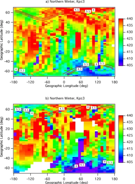
Figure 4a and b shows P at northern winter, at low and high magnetic activity. The same features described in Fig. 3 can be seen here, but the picture is less clear because of the slightly poorer sample statistics. Again, P increases from summer to winter (south to north), but the peak value ap-pears less well aligned with the magnetic L-values. During disturbed conditions, P is reduced at high magnetic latitudes in the southeast (summer) sector, as before, and to some ex-tent in northern (winter) high latitudes, too, but the displace-ments of the peak in P cannot be resolved because of small sample numbers.
Figure 5a and b shows P at low and high magnetic activ-ity at spring and fall equinox. These two seasons are suf-ficiently similar to be combined, and are fairly symmetrical
H. Rishbeth et al.: Variations of thermospheric composition 445
Fig. 3. AE-C: Maps of P -parameter for northern summer for (a) quiet magnetic conditions (Kp≤3 above) and (b) disturbed magnetic
conditions (Kp≥3, below). Red curves show magnetic L-values.
with respect to the edge of the auroral zones, particularly in disturbed conditions. The effect of magnetic activity is to increase P at low latitudes and decrease the minimum val-ues in the auroral zones. The detailed variations with latitude and longitude are due partly to the geomagnetic field config-uration, but they may also be influenced by seasonal varia-tions that are not entirely removed by averaging over the four equinox months, in addition to the effects arising from the limited bin samples mentioned in Sect. 2.2. There remains a possibility of genuine regional differences in composition, on top of the above, but more study would be needed to es-tablish their reality.
Figures 3 and 4 clearly illustrate that peaks in the P -parameter occur in the winter hemisphere at longitudes where the auroral oval is at its highest geographic latitude. This is most obvious in the south (Fig. 3a and b), where the
magnetic dip pole is at lower geographic latitude than in the north (67◦S as compared to 78◦N), but is also seen in north-ern winter (Fig. 4a). The minimum values of P occur in the summer hemisphere, near the longitudes where the auroral zone is at its lowest latitude. We do not show maps in mag-netic coordinates, because at higher southern latitudes there is a large data gap at longitudes 30–90◦W where the satellite does not reach high L-values.
If we take P as an indicator of thermospheric upwelling and downwelling, the plots suggest that upwelling exists at high magnetic latitudes, strongly in summer and weakly in winter, too, and is enhanced by magnetic activity (northwest corner of Fig. 3b, southeast corner of Fig. 4b). At both sol-stices, the winter zone of strongest downwelling (the greatest P-values and the most atomic thermosphere) is also magneti-cally aligned. It lies at L-values of 2.5–3 (magnetic latitudes
Fig. 4. AE-C: Maps of P -parameter for northern winter for (a) quiet magnetic conditions (Kp≤3 above) and (b) disturbed magnetic
conditions (Kp≥3, below). Red curves show magnetic L-values.
51–55◦), equatorward of the auroral zones, as predicted by Duncan (1969).
4 AE-C and CTIP maps of P -parameter vs. month and longitude
Figure 6 displays the data and model results in plots of P versus month and longitude at low magnetic activity, to show how the variations of composition vary throughout the year in five broad zones of latitude. There is some overlap, in that December is shown twice (months 0 and 12) and so is January (months 1 and 13). AE-C data are on the left, CTIP model results on the right. Not surprisingly, the CTIP results are fairly smooth, and lack much of the detail shown by the AE-C data.
The colour ranges are chosen to encompass the full sea-sonal variation seen in the satellite data and the model data. A slight difference between their scales facilitates a compar-ison over latitude within a data set, with a little compromise to the comparison of features seen in the satellite and model data. If we use the same colour scale for every panel, the five AE-C panels are noticeably bluer in colour (indicating lower P-values) than the five corresponding CTIP panels. To ad-just the colour scales to obtain a better colour match between the two sets of panels, we first computed the mean value of P for all ten panels, with the following results for the five latitude ranges (north to south, rounded to nearest integers):
– AE-C: 425, 426, 431, 427, 423; mean 427; – CTIP: 450, 443, 438, 441, 443; mean 443.
H. Rishbeth et al.: Variations of thermospheric composition 447
Fig. 5. AE-C: Maps of P -parameter for equinox (March, April, September, October) for (a) quiet magnetic conditions (Kp≤3, above) and
(b) disturbed magnetic conditions (Kp≥3, below). Red curves show magnetic L-values.
The difference between the overall mean AE-C and mean CTIP values is 443 − 427 = 16, which is the adjustment we made in the colour scales. The mean values of P for the data and the model now match quite well in colour, but the range of P is smaller in the data than in the model, and the highest P-values in the AE-C panels only reach orange colours, as compared to the reds in the CTIP panels.
4.1 Mid-latitudes
At 50–70◦N (top row), where summer months are in the cen-tre of the panels and winter months are at the top and bottom, the summer/winter variation stands out strongly. Both sum-mer and winter values of P are greater in eastern longitudes than in western. The lowest summer values of P are found at Pacific longitudes 130–180◦W in the data, but further east in
the model at Atlantic/American longitudes 0–100◦W. CTIP clearly overestimates the winter values of P ; this indicates that the winter downwelling, which increases P , is less pro-nounced in the AE-C data than in CTIP. At 30–50◦N the sea-sonal variations are smaller, both in data and model, but are in the same sense as at 50–70◦N. Again, the summer mini-mum is over the Pacific in the data, but over the Atlantic in the model.
Turning to southerly mid-latitudes (two bottom rows of Fig. 6), summer months are at the top and bottom of the pan-els and winter months in the centre. At 30–50◦S the summer minima in the AE-C values are now in east longitudes in the African/Indian Ocean sector, 30–80◦E. In west longitudes, greatest P tends to occur around or after equinox (April and October), giving a semiannual pattern superimposed on the winter/summer variation. The semiannual tendency also
ap-Fig. 6. P -parameter from AE-C data (left) and CTIP (right) vs. month and longitude for Kp≤3, for five ranges of geographic latitude. Top
H. Rishbeth et al.: Variations of thermospheric composition 449
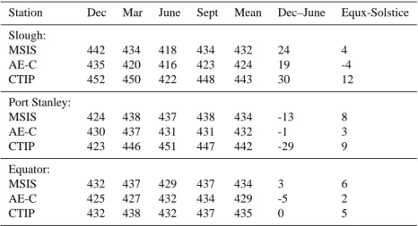
Table 1. P -parameters at midday from models and data.
Station Dec Mar June Sept Mean Dec–June Equx-Solstice Slough: MSIS 442 434 418 434 432 24 4 AE-C 435 420 416 423 424 19 -4 CTIP 452 450 422 448 443 30 12 Port Stanley: MSIS 424 438 437 438 434 -13 8 AE-C 430 437 431 431 432 -1 3 CTIP 423 446 451 447 442 -29 9 Equator: MSIS 432 437 429 437 434 3 6 AE-C 425 427 432 434 429 -5 2 CTIP 432 438 432 437 435 0 5
pears weakly in western longitudes in the AE-C panel for 50–70◦S, but rather as a broad plateau extending from au-tumn (months 3–4) to spring (months 9–10). In the southern CTIP panels, any semiannual tendency is hidden by the un-realistically high mid-winter maxima of P .
Though not shown here, the distributions of P plotted in magnetic L-coordinates are quite similar at mid-latitudes to those in geographic coordinates but, as previously remarked, they lack complete longitude coverage at high latitudes in the south.
4.2 The equatorial zone
The centre row of Fig. 6 shows the equatorial zone, between 20◦S and 20◦N geographic. The range of P -values through-out the year is smaller than at mid-latitudes, particularly in the CTIP panel where the range is <10. The semiannual variation in the CTIP results (right), of about 5 units, ap-pears very weakly in the AE-C data (left). In western lon-gitudes the AE-C plot shows an annual variation of about 5 units in P , with maximum in November–February and min-imum in June–August. The hemispheric differences may be connected with differences in the magnetic latitude, since in the American sector the magnetic equator is south of the ge-ographic equator and the data in Fig. 6 come mostly from north magnetic latitudes. Conversely, in the Asian equatorial sector the data come mostly from south magnetic latitudes.
A plot of the AE-C P -values for the magnetic equato-rial zone (Rishbeth, 2003), covering magnetic latitudes 20◦– 20◦N, also shows a strong annual (December–June) varia-tion of P in most longitudes, which tends to conceal any semiannual pattern. However, at 60◦–90◦E the pattern is weakly semiannual. The greater strength of the annual pat-tern in the “magnetic” plot may be attributed, at least partly, to summer/winter differences of composition, bearing in mind that the “magnetic equatorial zone” extends into ge-ographic midlatitudes in some longitude sectors.
As discussed by Rishbeth et al. (2000), the equinox max-ima of P indicate that the thermosphere is less disturbed at equinox than it is at solstice, when solar input is continuous at high summer latitudes and drives the strong summer-to-winter circulation (Fuller-Rowell, 1998).
5 Comparisons of AE-C, CTIP and MSIS values of
P-parameter
We used the MSIS-86 model (Hedin, 1987) to compute the P-parameter from Eq. (A4) for Slough (52◦N, 1◦W) and
Port Stanley (52◦S, 58◦W), for solar 10.7 cm flux of 100
units and low magnetic activity (Ap = 4). We found that,
as expected, P is almost height-independent above 200 km, while from 200 km down to 120 km it increases by about 7 units. In contrast, using the more complete formula (A3), P is virtually height-independent down to 150 km, and de-creases by only about 5 units from 150 to 120 km. At 300 km height, we found that MSIS P is smaller at midnight than at noon, but only by about 4 units, which supports our deci-sion (Sect. 2.2) to use all local times in analysing the AE-C data. We also used MSIS to compute P for an “equator” point near (0◦, 40◦W), which is approximately where the geographic and magnetic equators cross (the MSIS values at 0◦, 160◦W, the other longitude where the equators cross, are just 1 unit lower than at 40◦W). Table 1 shows the noon
values of P at these places from the MSIS and CTIP mod-els and the AE-C data for December and June solstices and March and September equinoxes. In the case of AE-C, the data are averages over an area within 5◦of the required point, to remove some of the point-to-point variations. Consider the means of the four seasonal values of P , shown in the column headed “Mean”. At Slough and Port Stanley, these CTIP means are markedly higher than the others, except in local summer, which implies that the CTIP thermosphere is too atomic (recall that each unit of P corresponds to about 5% in the O/N2ratio). This is mainly because CTIP gives too big a
winter/summer variation, especially at Port Stanley. At Port Stanley and at the equator, the semiannual (equinox/solstice) variation in the AE-C data is much smaller than that given by MSIS and CTIP; at Slough the equinox/solstice difference in the AE-C and MSIS values of P is small and not signifi-cant, with the larger difference in CTIP being due to the small summer value of P . In most cases the March and Septem-ber values of P are equal or nearly so, with the exceptions of the AE-C data for Port Stanley (greater in March) and at the equator (greater in September). Since the AE-C data were used in constructing the MSIS model, we might expect the MSIS and AE-C values of P to agree, but we have no expla-nation as to why they do not, beyond the slight overestimate of the atomic oxygen concentration mentioned in Sect. 2.1.
At the equator, MSIS and CTIP agree well, with a marked semiannual variation not seen in the AE-C values, which peak in September. The annual variation is not promi-nent in the AE-C data at longitudes around 35◦W, and the (December–June) difference may not be typical of low lat-itudes generally; in any case the data in this vicinity have rather poor statistics.
6 Discussion
The most obvious result is that, in both hemispheres but especially the north, the O/N2 ratio and the derived P
-parameter are greater in winter than in summer at all lon-gitudes, denoting substantial seasonal changes in the neutral atomic/molecular composition. We find that the MSIS atmo-sphere is more atomic than the AE-C data indicate, typically by about 5 units of P , corresponding to a difference of about 30% in the O/N2ratio. On the other hand, the CTIP
compu-tations give a substantially more molecular atmosphere than the AE-C data indicate; at northern mid-latitudes (Slough) the seasonally averaged difference amounts to about 20 units of P , which corresponds to a difference of about 3:1 in the O/N2 ratio. We do not pursue the reasons for these
differ-ences.
With the level of smoothing we used, the coverage of lati-tude and season is reasonably complete. The general patterns of the O/N2 ratio and the P -parameter are similar (Fig. 2),
but the P -parameter is much more useful, because it enables data from a great range of height to be combined. Omitting the temperature term in the P -parameter (Eq. A4) avoids dif-ficulties with incomplete temperature data, without seriously affecting the most valuable property of P , namely its inde-pendence of height.
The “winter downwelling” and its effects on the O/N2
ra-tio and NmF2 are well displayed by CTIP modelling. Ac-cording to Duncan (1969), the downwelling zones are just equatorward of the auroral ovals. Consequently, the situation in longitude sectors adjacent to the (geographic) longitudes of the magnetic poles (which we call “near-pole” longitudes) differs from that in sectors remote from the (geographic) lon-gitudes of the magnetic poles (which we call “far-from-pole” longitudes) (Rishbeth and M¨uller-Wodarg, 1999; Rishbeth et
al., 2000). In “near-pole” longitudes, the downwelling zones are at relatively low geographic latitudes (around 50◦), which
are sunlit at noon in mid-winter (though at large solar zenith angles), and winter NmF2 is large because of the high O/N2
ratio. But in “far-from-pole” longitudes, the downwelling zones are at high geographic latitudes and receive little or no direct sunlight in winter. So the electron density is very low at mid-winter, despite the high O/N2ratio, and this accounts
for the tendency towards equinoctial (semiannual) maxima of NmF2 in “far-from-pole” longitudes.
These features appear in CTIP noon maps, Fig. 5 of Zou et al. (2000), in which the high latitude areas of depressed
NmF2 are centred about 70◦N, 90◦E geographic in Decem-ber and 70◦S, 90◦W in June. Although the satellite did not reach latitudes of total winter darkness, the AE-C data do show high values of P -parameter (large O/N2ratio) in these
longitudes at latitudes above 60◦, especially in the north (Figs. 3 and 4), as predicted by CTIP. Clearly, composition data from higher latitudes are needed to confirm our interpre-tation.
However, the summer/winter range of P is clearly greater in the model than in the data. Winter P -values in CTIP are too large because the model overestimates the downwelling there, the reason being that the model lacks any mechanism, such as an additional heating source, for generating sufficient upwelling in winter. This lack is most noticeable in regions where there is no sunlight at all, but it has little effect in the summer hemisphere or at equinox. Obviously, downwelling and upwellling must balance globally; but our results suggest that the winter downwelling is actually less intensive, and must, therefore, be more widely distributed than is portrayed by CTIP.
We should note that our CTIP simulations do not consider the effects of tidal forcing from below. Tides generated in the troposphere and stratosphere propagate into the lower ther-mosphere, dissipating their energy at 100–150 km altitude, thus releasing considerable amounts of momentum and en-ergy into the region. This may generate additional upwelling at mid-latitudes, thus potentially reducing the O/N2ratio and P in the winter hemisphere – a possible reason for the dis-crepancy between CTIP and MSIS.
The AE-C maps (Figs. 3–5) show some alignment with magnetic L-shells, which also appears in the CTIP results. This is not surprising, since the model is driven by high lat-itude energy inputs as well as by solar heating. However, it is probably not useful to relate the CTIP maps in detail to L-values. Our version of CTIP relies entirely on the sta-tistical high latitude inputs, as given empirically by Foster et al. (1986) (from averages of Millstone Hill observations of convection fields) and by Fuller-Rowell and Evans (1987) (from Tiros satellite data on particle precipitation). These are limited data sets that have undergone much processing, including averaging over many seasons and binning with Kp. Finally, the CTIP profiles are smooth because the model
omits any physical processes of fine spatial scale or short time-scale. The only source of short-term variability in CTIP
H. Rishbeth et al.: Variations of thermospheric composition 451 is the diurnal variation of solar heating; even the magnetic
forcing is UT-independent.
7 Conclusions
1. The AE-C data show strong seasonal variations of neu-tral composition, with greatest P -parameter and O/N2
ratio in winter near solstice, though not necessarily at solstice.
2. The solstice maps show that P , and, therefore, the O/N2
ratio at fixed pressure-levels, increases steadily from summer to winter.
3. The AE-C data confirm fairly well the results of the CTIP modelling of Rishbeth et al. (2000), which indicate strong summer/winter variations of the P -parameter (O/N2 ratio) in longitude sectors near the
magnetic poles, but a tendency towards equinoctial maxima of P elsewhere. In the data, however, semi-annual variations of P appear weak, except perhaps in western mid-latitudes in the Southern Hemisphere. 4. Magnetic disturbance decreases P at high latitudes.
There are smaller effects at midlatitudes, namely some decrease in summer and a small increase in winter, consistent with the well-known seasonal variations of F2-layer disturbances. We have not studied individual storms.
5. We combine data from all local times, and, therefore, cannot discuss local time effects in detail; but by com-paring daytime values of P with values for all local times, we found that the composition does not vary greatly from day to night. This agrees with CTIP mod-elling by Rishbeth and M¨uller-Wodarg (1999), which gave day-to-night changes in P of only about 5 (their Fig. 2), consistent with the time constant for composi-tion changes, which is estimated to be of the order 20 days (Rishbeth et al., 2000). The MSIS day-to-night changes of P , too, are typically 5 units.
6. The CTIP model overestimates the winter increases in the P -parameter (or O/N2 ratio) produced by
down-welling at high winter mid-latitudes, more so in the south than the north. This implies that the model lacks some process, such as an additional energy source, which opposes the downwelling in the winter hemi-sphere.
7. Values of the P -parameter computed from the MSIS model, for places at northern and southern mid-latitudes, broadly agree with values given by AE-C, but in general portray a more molecular thermosphere than do the AE-C data, while the CTIP thermosphere is rather more molecular than is shown by MSIS. This may imply some systematic error in the derived O/O2
ratios, but we do not attempt to pursue the matter in this paper.
8. The latitude/longitude maps give no evidence of any equatorial effect in thermospheric composition, so com-position plays no part in forming the F2-layer equatorial anomaly.
In summary, we have shown that the NATE data from the AE-C satellite provide a useful means of investigating thermospheric composition; these data show marked win-ter/summer variations of composition, which broadly con-firm the “composition change” theory of F2-layer seasonal and magnetic storm variations, and the results agree quite well with both the theoretical CTIP and empirical MSIS models of the thermosphere with regards to the mean compo-sition, though not necessarily in the details of its variations. Acknowledgements. We wish to thank the National Space Science
Data Centre A for providing the AE-C unified abstract data. The work at UT Dallas is supported by NASA grant NAG 5-10271. IM-W was funded by the British Particle Physics and Astronomy Research Council (PPARC) grant PPA/G/O/1999/00667 and since 2002 by the British Royal Society. All CTIP model calculations were carried out on the High Performance Service for Physics, Astronomy, Chemistry and Earth Sciences (HiPer-SPACE) Silicon Graphics Origin 2000 Supercomputer located at University College London and funded by PPARC.
Topical Editor M. Lester thanks C. Fesen and R. Balthazor for their help in evaluating this paper.
Appendix A The compositional P -parameter
To overcome the difficulty that the O/N2 ratio varies
rapidly with height, we express our results in terms of the “P -parameter”, much as defined by Rishbeth and M¨uller-Wodarg (1999). Let ζ denote “reduced height”, measured from a base height ho in units of the pressure scale height of atomic hydrogen. This scale height is given by H1=RT /g,
and is about 1000 km, where R is the universal gas constant, T is temperature, and g is the gravitational acceleration (as H1varies with height, the relation between Z and the real
height h involves an integration, but this is a detail we need not consider here).
The base height ho is at around 120 km, above which height the gases O and N2may be assumed to be distributed
with their own scale heights in the ratio 28/16. Let the suf-fix “o” denote values of parameters at the base level ho. In terms of natural logarithms, the gas concentrations vary with height above ho according to the equations:
ln[O]= ln(T o/T ) + ln[O]o−16ζ (A1)
ln[N2]= ln(T o/T ) + ln[N2]o−28ζ. (A2)
Multiplying Eq. (A1) by 28 and Eq. (A2) by 16, and subtract-ing to cancel the terms in ζ , we have
28 ln[O]−16 ln[N2] +12 ln T =P
The left-hand side of Eq. (A3) is the P -parameter, as defined by Rishbeth and M¨uller-Wodarg (1999). The numerical val-ues of P depend on the O/N2ratio and also on the units of
concentration (here m−3). The relation between P and ln [O/N2] is not quite linear, and depends weakly on the O/N2
ratio. For the O/N2 ratios prevalent at the F2-peak, a 5%
increase in the O/N2 ratio corresponds to a change in P by
about +1 unit. Larger changes in P , for example, by 10 and 25 units, change the O/N2ratio by factors of about 1.8 and 4,
respectively.
The temperature term 12 ln T is not particularly important and, as explained in Sect. 2.3, we omit it for the purposes of this paper. Instead, we take
P =28 ln[O]−16 ln[N2]. (A4)
This modified P is not exactly height-independent, because the temperature term 12 ln T in Eq. (A3) changes by 1.2 if the temperature changes by 10%. However, this has lit-tle effect on our results. According to the empirical MSIS model (Hedin, 1987), for the range of solar activity spanned by our AE-C data and for moderate geomagnetic activity (Kp<3), the temperature at F2-layer heights (not much
dif-ferent from the “exospheric temperature”) varies at mid-latitudes by about 30% between day and night and 20% between summer and winter. These temperature changes cause our “simplified P ” to vary by about ±1.8 diurnally and ±1.2 seasonally. In comparison, the seasonal and latitudinal changes of P span some tens of units, so the temperature term does not appreciably contribute to these variations.
References
Berkner, L. V., Wells, H. W., and Seaton, S. L.: Characteristics of the upper region of the ionosphere, Terr. Magn. Atmos. Elect., 41, 173–184, 1936.
Dalgarno, A., Hanson, W. B., Spencer, N. W., and Schmerling, E. R.: The Atmospheric Explorer Mission, Radio Sci., 8, 263–266, 1973.
Duncan, R. A.: F-region seasonal and magnetic storm behaviour. J. Atmos. Terr. Phys., 31, 59–70, 1969.
Foster, J. C., Holt, J. M., Musgrove, R. G., and Evans, D. S.: Iono-spheric convection associated with discrete levels of particle pre-cipitation, Geophys. Res. Lett., 13, 656–659, 1986.
Fuller-Rowell, T. J.: The “thermospheric spoon”: A mechanism for the semi-annual density variation, J. Geophys. Res., 103, 3951– 3956, 1998.
Fuller-Rowell, T. J. and Evans, D. S.: Height-integrated Pedersen and Hall conductivity patterns inferred from the TIROS-NOAA satellite data, J. Geophys. Res., 92, 7606–7618, 1987.
Fuller-Rowell, T. J., Rees, D., Quegan, S., Moffett, R. J., Codrescu, M. V., and Millward, G. H.: A coupled thermosphere-ionosphere model (CTIM), in: STEP Handbook of Ionospheric Models, edited by Schunk, R. W., Utah State University, Logan, Utah, 217–238, 1996.
Hedin, A. E.: MSIS-86 thermospheric model, J. Geophys. Res., 92, 4649–4662, 1987.
Mauersberger, K., Kayser, D. C., Potter, W. E., and Nier, A. O.: Seasonal variation of neutral thermospheric constituents in the northern hemisphere, J. Geophys. Res., 81, 7–11, 1976. Millward, G. H., Rishbeth, H., Moffett, R. J., Quegan, S., and
Fuller-Rowell, T. J.: Ionospheric F2-layer seasonal and semian-nual variations. J. Geophys. Res. 101, 5149–5156, 1996a. Millward, G. H., Moffett, R. J., Quegan, S., and Fuller-Rowell,
T. J.: A coupled thermosphere-ionosphere-plasmasphere model (CTIP), in: STEP Handbook of Ionospheric Models, edited by Schunk, R. W., Utah State University, Logan, Utah, 239–280, 1996b.
Rishbeth, H.: Questions of the equatorial F2-layer and thermo-sphere, J. Atmos. Solar-Terr. Phys., accepted, 2003.
Rishbeth, H. and Setty, C. S. G. K.: The F-layer at sunrise, J. Atmos. Terr. Phys., 21, 263–276, 1961.
Rishbeth, H. and M¨uller-Wodarg, I. C. F.: Vertical circulation and thermospheric composition: a modelling study, Ann. Geophysi-cae, 17, 794–805, 1999.
Rishbeth, H., M¨uller-Wodarg, I. C. F., Zou, L., Fuller-Rowell, T. J., Millward, G. H., Moffett, R. J., Idenden, D. W., and Aylward, A. D.: Annual and semiannual variations in the ionospheric F2-layer: II. Physical discussion, Ann. Geophysicae, 18, 945–956, 2000.
Spencer, N. W., Niemann, H. B., and Carignan, G. R.: The neutral-atmosphere temperature experiment, Radio Sci., 8, 287–296, 1973.
Torr, M. R. and Torr, D. G.: The seasonal behaviour of the F2-layer of the ionosphere, J. Atmos. Terr. Phys., 35, 2237–2251, 1973. von Zahn, U., Fricke, K. H., and Trinks, H.: Esro 4 gas analyzer
results, I. First observations of the summer argon bulge, J. Geo-phys. Res., 78, 7560–7562, 1973.
Yonezawa, T.: The solar-activity and latitudinal characteristics of the seasonal, non-seasonal and semi-annual variations in the peak electron densities of the F2-layer at noon and at midnight in mid-dle and low latitudes, J. Atmos. Terr. Phys., 33, 889–907, 1971. Zou, L., Rishbeth, H., M¨uller-Wodarg, I. C. F., Aylward, A. D.,
Millward, G. H., Fuller-Rowell, T. J., Idenden, D. W., and Mof-fett, R. J.: Annual and semiannual variations in the ionospheric F2-layer: I. Modelling, Ann. Geophysicae, 18, 927–944, 2000.