View of An orthotropic incremental model for the hydromechanical behaviour of softwood

(1)

First International Conference on Bio-based Building Materials June 22nd_{- 24}th₂₀₁₅ Clermont-Ferrand, France

AN ORTHOTROPIC INCREMENTAL MODEL FOR THE HYDROMECHANICAL

BEHAVIOUR OF SOFTWOOD

S.L. Nguyen1,2_{*, J.F. Destrebecq}1,2

1_{Blaise Pascal University, Pascal Institute, BP 10448, Clermont-Ferrand, France} 2

CNRS, UMR 6602, Pascal Institute, Aubière, France * Corresponding author; sung-lam.nguyen@ifma.fr

Abstract

In the present work, a 3D orthotropic model is developed, aiming at precisely predicting the hydromechanical behavior of timber structures. Based on test results and on thermodynamical considerations, an evolution law is proposed for the hydro-lock strain. This phenomenon is assumed to occur in the longitudinal direction, but not in the tangential and radial directions. Beside, a 3D incremental formulation is developed to depict the viscoelastic strain at variable humidity, what allows overcoming the memory effect. Finally, the coupling of these two parts leads to a new 3D incremental model suitable to simulate the time dependent hydromechanical behavior of softwood. It should be noted that the time step to be used for numerical simulations must be finite, but not necessarily small. This important feature significantly reduces the computational effort while maintaining good accuracy. For the sake of illustration, the model is finally used to simulate the effect of varying humidity on the evolution of stress and strain states in a plain wood beam loaded in axial tension and in bending.

Keywords:

Wood; mechanosorptive effect; viscoelasticity; hydro-lock effect; incremental formulation.

1 INTRODUCTION

The behavior of softwood material is governed by complex interactions between mechanical stress and moisture content variations, called mechanosorptive effect. This effect can produce structural failure, even in the case of small load [Hearmon 1964]. Therefore, many research works have been performed, aiming at explaining or modeling this complex behavior.

Some authors proposed to describe this phenomenon as a hydrolock effect, which is considered a temporary locking of the mechanical strain during a period of drying [Gril 1988], [Dubois 2005], [Husson 2010]. A recent study based on specific mechanosorptive tests [Saifouni 2014] confirmed the existence of a hydrolock strain resulting from a locking effect in the longitudinal direction. No evidence of the existence of a hydrolock effect in transverse directions was reported. Besides, these authors also developed models to simulate this effect, but with a limitation to 1D case, which makes them not easily suitable to depict the hydromechanical response of a wooden structure in environmental conditions.

In this context, we propose a new model for the hydromechanical behavior of softwood, which takes into account the coupling between hydrolock and orthotropic viscoelastic effects. In a first part, based on

hydrolock strain as a base for the modeling. Then, from thermodynamical considerations, evolution laws for the hydrolock strain and the viscoelastic strain are proposed in the second part. An incremental numerical model will be developed then. Finally, we present and discuss exemplary simulation results.

2 PROPERTIES OF HYDROLOCK STRAIN The process of creation and recovery of hydrolock strain was evidenced in an experimental program, what was especially dedicated to the study of the mechanosorptive behavior of silver fir specimens (Abies alba Mill.) [Saifouni 2014].

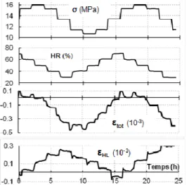
In this study, a mechanosorptive tensile test in longitudinal direction was carried out on small scale specimens under cyclic loading and humidity. The stress and the relative humidity were varied stepwise, in such a way as to describe a sinus-like diagram (Fig. 1). The elementary contributions of the hydric, the elastic and the viscous effects to the resulting total strain were estimated from a series of preliminary tests. By subtracting these elementary contributions from the total resulting strain recorded during the test, it was finally possible to evidence the existence of a hydro-lock strain as a result of the complex interaction between the mechanical stress and the humidity variations. The resulting evolution of the hydro-lock

(2)

Fig. 1. Hydromechanical loading, total measured strain and evidenced hydro-lock strain.

The main feature can be summarized as follows: i) the hydro-lock strain is created and develops instantly for each decrease of humidity in the drying phase under constant stress ; its evolution consists of a series of successive steps. ii) a stress variation at constant humidity

does not cause any change in the hydro-lock strain. Moreover, this strain may be considered constant when the relative humidity does not vary. In other words, the hydro-lock strain is independent of time and stress variations at constant relative humidity.

iii) the hydro-lock strain (when it exists) decreases in absolute value, until it disappears when the moisture content returns to its initial value at the beginning of the drying phase under stress.

These three important features will be considered below for the construction of a new hydrolock viscoelastic model.

3 SETTING OF THE ANALYTICAL MODEL The model bases on the hypothesis of the total strain partition [Saifouni 2014], as follows:

w ve HL e

t ε ε ε ε

ε& =& +& +& +& (1)

is the elastic strain. is the hydrolock strain. is a free strain which depends on the shrinkage-swelling coefficients and the moisture content. is a pure viscoelastic strain which depends on the level and duration of loading. This hypothesis can be schematized by an analogue model, as follows:

e

ε

_HL

ε

ve

ε

w

Fig. 2: Analogue model.

Accordingly, each of elementary contributions to the total strain is analyzed separately in the following. Their sum will finally yield the complete model.

3.1 Free and elastic strain parts

The free strain evolution simply writes as follows:

w

&

α

ε

=

(2)

where is a swelling/shrinkage coefficient that is considered constant in this work.

The elastic strain is given by Hooke’s law with depending on moisture content of the Young’s modulus. Hence













_′

−

+

=

+

=

ε

σ

ε

σ

w

E

w

E

w

E

w e e e

&

)

(

)

(

)

(

2 (3)

where is the elastic strain evolution due to the varying stress , and is the one due to the varying elasticity modulus caused by the moisture content changes .

3.2 Hydrolock strain part

The validity of equation (1) and the analogue model must be justified in the thermodynamic framework.

Thermodynamic framework

The justification bases on the choice of a thermo-dynamical potential, as a function of state variables. In the present case, the state variables necessary to describe the reversible instantaneous hydroelastic behavior at constant temperature (ignoring the viscous effects) are the strain and the moisture content . To describe the hydrolock effect of the strain in the drying phase under stress, it is necessary to introduce an additional state variable . The thermodynamical potential is decomposed in two parts, as follows:

(

ε wεHL

)

ψe

(

ε w

)

ψHL

(

εHL

)

ψ , , = , + (4)

The third state law provides a relationship between the additional state variable and its associated variable

, as follows

(

HL

)

HL HL HL g d d ε σ ε ψ ε ψ σ = ⇒ = ∂ ∂ = ~ ~ ₍₄₎

In this equation, is a fictitious stress without specified significance. Equation (4) shows the existence a bi-univocal relationship between and , which can also be written

( )

σ

ε_HL = g−1 ~ (5)

Expressions for the hydrolock strain need be specified, which will be done in the following sections for drying and wetting phases, respectively.

Hydrolock strain evolution in the drying phase

In equation (1), the sum can be written

HL w e e HL e

ε

&

+

&

=

&

σ

+

&

+

&

(6)

As mentioned above as feature (i) in section 2, the test results showed that the hydrolock strain results from a blocking effect of strain in the drying phase under stress. If there isn’t stress variation , it comes from equation (6)

(

)

0

0 + + ₀ =

<

∀w& ε&σe ε&ew ε&HL _σ_&₌ (7)

(3)

σ ε ε w w E w E w e w HL & & & & ₍ ₎ ) ( 2 0 ′ = − = < (8)

Where present the evolution of the hydrolock strain in the drying phase. Equation (8) shows that the blocking phenomenon of the strain during a drying phase is due to the evolution of the hydrolock strain which compensates the part of the elastic strain variation due to the Young’s modulus evolution. This equation also shows that the hydrolock strain does not change at constant humidity , regardless of the mechanical stress . This property is in agreement with experimental observations (feature (ii) in section 2).

Hydrolock strain evolution in the wetting phase

The tests showed that the hydrolock strain (if it exists) decreases in absolute value during the wetting phase until it disappears when the moisture content returns to its initial value at the beginning of the drying phase under stress (feature (iii) in section 2). This indication is not enough to express the hydrolock strain in the humidification phase. Another possibility is to assume that its evolution is similar to the equation (8). But we see that this equation doesn’t allow the hydrolock strain to recover if the stress is zero or insufficient. To overcome this problem, we replace the mechanical stress in equation (8) by a fictitious stress to determine. This leads to

σ ε ~ ) ( ) ( w w E w E w HL & & _& 2 0 ′ = > (9)

where is the evolution of the hydrolock strain in the wetting phase. To satisfy the remark above, the hydrolock strain must disappear when . Hence, the actual value of the fictitious stress is obtained by integrating equation (9) on the interval with the boundary condition , which yields

HL w E w E w E w E ε σ ) ( ) ( ) ( ) ( ~ − = (10)

It can be noticed that this expression is the function introduced in equation (4).

Finally, all of equations (8), (9) and (10) established the analytical formulation of the hydrolock strain evolution, in accordance with experimental evidences and with the principles of thermodynamics. It is worth noticing that the value of the fictitious stress only depends on the accumulated amount of hydrolock strain at the time considered. Its value is always defined . The introduction of this fictitious stress allows solving the recovery of the hydrolock strain in a moistening phase, regardless of the loading level. Furthermore, we note that it was not necessary to specify the physical meaning of the fictitious stress to establish the equations above.

3.3 Viscoelastic strain part

The viscoelastic part in the analogue model is schematized by a Kelvin’s cell parallel to a Maxwell’s branch (Fig.2). This elementary model depicts a pure viscoelastic behavior (no instantaneous elasticity). Hence, the hydrolock effect doesn’t influence on time dependent strain part (feature (ii) in section 2). Combined with a spring in series, this pure viscoelastic model is equivalent to Maxwell’s generalized model containing two elementary Maxwell’s branches plus an

viscoelastic and elastic part will be merged in the Boltzmann’s equation in the case of relaxation. The relaxation function is required to solve the viscoelastic problem. In the following, the relaxation function is approximated by a Dirichlet’s series, in which the coefficients depend linearly on moisture content as follows

(

)

∑

( )

( ) = − −

≅

r t t

e

w

t

r

0 0 0 µ β µ µ

γ

,

(11)

where are fixed constants; is the moisture content at time . Linear laws are assumed for the parameters in order to depict the dependency of the relaxation function towards the moisture content . The set of constants and can be determined from tests using the least square method.

In the general orthotropic case, the viscoelastic matrix of relaxation has 9 independent functions, which depend on the moisture content level , the loading time and the actual time . This number reduces to six for the case of constant Poisson’s coefficients. From a close inspection of test results in [Carriou 1987], it was concluded that the number of functions can be reduced to two only, the one for the three shear terms, the second for the other terms. Hence, we can write

(

)

[

R

t

,

t

₀

,

w

]

=

[

ρ

(

t

,

t

₀

,

w

)

]

[

A

( )

w

]

(12) where, is the elasticity rigidity matrix, which depends on the actual moisture content at time . is a diagonal matrix containing two relaxation functions represented by Dirichlet’s series such as equation (11),

where . Hence,

( )

[

]

( ) ( ) ( ) ( ) ( ) ( )













=

2 2 2 1 1 1

0

µ µ µ µ µ µ µ

γ

w

(13) where , and

[

]

( )

_{[ ]}

1 0 t t e exp = −βµ − µ (14)

These equations mean that the three shear terms of the viscoelastic matrix evolve proportionally to the second dimensionless function, and the nine other terms evolve proportionally to the first one. Let us note that and above represent a vector and a matrix, respectively.

4 INCREMENTAL NUMERICAL MODEL Using an incremental form is a good way to solve a time dependent problem. An incremental form for a behavior law is a relation between strain and stress increments on a finite time interval. Thanks to the

(4)

step-by-step calculation, it is not necessary to memorize the total stress and strain histories.

By taking into account the hypothesis of strain partition above (see section 3), the incremental total strain is equal to the sum of its elementary parts, as follows:

{ } {

∆εt = ∆εe

} {

+ ∆εHL

} {

+ ∆εve

} {

+ ∆εw

}

(15)

The incremental forms of the four parts of equation (15) are established in the following.

4.1 Incremental form of the free strain

According to equation (2), the incremental free strain simply depends on incremental moisture content and the swelling/shrinkage coefficients matrix, which is assumed constant in the paper:

{

∆ε_w

}

=

[ ]

α∆w (16)

4.2 Incremental form of the hydrolock strain This point is treated separately for the two phases of drying and moistening with the following notations:

, , ,

and . It should be noted that the hydrolock effect exists only in the longitudinal direction. Therefore, the Young’s modulus here is the one in this direction. For the sake of simplicity, we note here that are a matrix 6x6 and a column vector 6x1 the longitudinal direction term is equal to 1 and the other terms are equal to zero.

Drying phase

As mentioned in section 3.1, the varying hydrolock strain in the drying phase compensates the elastic strain variation at constant stress (equation (8)). By taking advantage of this property, the increment can be obtained by integrating equation (8) over a finite time interval with a hypothesis of linear modulus variation on this time interval. It leads

{

∆ε_HL

}

=k_d

{ }

1 (17) with

(

)

(

)

        + + + + = 2 2 2 1 1 2 2 E E E E E E E k_d _L L ∆ ∆ σ σ ∆ ∆ ∆ (17’) are the stress and its increment in the longitudinal direction.

Wetting phase

In this case, the hydrolock strain increment is obtained by integrating of in equation (9). Replacing equation (10) in (9) and then resolving a first order differential equation gives

{

}

₍

₎

(

)

{

HL

}

HL E E E E E E ε ∆ ∆ ε ∆ + − = (18)

Finally, the combination of equations (17) and (18) yields

{

∆εHL

}

=

[

ηHL

]

{ } {

∆σ + ξHL

}

(19) with

[

]

(

)

[ ]

{

}

(

)

{ }

               + + = + = < 1 1 1 2 1 2 0 2 2 2 E E E E E E E η w if L HL HL ∆ ∆ σ ξ ∆ ∆ & (20)

[

] [ ]

{

}

₍

₎

(

)

{

}

     + − = = > HL HL HL E E E E E E η w if ε ∆ ∆ ξ 0 0 & (21)

4.3 Incremental form of the elastic-viscoelastic strain

The sum of incremental elastic and viscoelastic strains will be derived from Boltzmann’s equation formulated in relaxation case:

( )

{ }

t =t∫

[

R

(

t w

)

]

{

_eve

( )

}

d 0 τ τ ε τ σ , , & (22)

where is the sum of elastic and pure viscoelastic strain (elastic-viscoelastic strain). Given equations (12-14), equation (22) can be written

( )

{ }

[

( )

]

[

( )

]

{

( )

}

( )

[

]

[

( )

]

[

(

)

]

{

( )

}

∑ ∫ − + + ∫ = = r t eve µ µ t eve d t exp w w A d w w A t 10 0 0 µ γ τ ε τ τ τ τ ε γ σ & & (23)

The incremental stress is defined as:

{ }

∆σ =

{

σ

(

t+∆t

)

}

−

{ }

σ

( )

t (24) By substituting equation (23) in equation (24) and after arrangement, we have

{

∆εeve

}

=

[

ηeve

]

{ } {

∆σ + ξeve

}

(25)

where,

[

]

₌

[

(

₊

)

]

[

(

₊

)

]

−1 w w w w C η_eve

∆

Γ

∆

(26) with

(

)

[

]

                    = + 2 2 2 1 1 1 0 0 0 0 0 0 0 0 0 0 0 0 0 0 0 0 0 0 0 0 0 0 0 0 0 0 0 0 0 0 Γ Γ Γ Γ Γ Γ ∆ Γ w w (27)

( )

₍

₎

( )

₍

₎

( )

₍

₎

( )

₍

₎

( )

         ∑ + − + + = ∑ + − + + = = − = − r t r t t e w w w w t e w w w w 1 2 2 2 0 2 1 1 1 1 0 1 2 1 1 1 µ _µ ∆ β µ µ _µ ∆ β µ ∆ β ∆ γ ∆ γ Γ ∆ β ∆ γ ∆ γ Γ µ µ (28)

{

}

= ∑

{

}

= r eve eve 0 µ µ ξ ξ (29)

(5)

{

}

[

(

)

]

[

( )

]

(

)

( )

(

)

[

w w

]

{

( )

t

}

w w w w C w w C eve 0 1 0 0 0 0 σ ∆ Γ γ ∆ γ ∆ ξ µ − + ×               ₊ − + = = : (30)

{

}

(

)

[

]

( )

[

]

(

)

( )

[

( )

]

(

)

[

w w

]

{

( )

t

}

t exp w w w w C w w C r _eve µ µ µ µ µ σ ∆ Γ ∆ γ ∆ γ ∆ ξ µ 1 1 − + ×                     ₊ − + = ÷ = : (31)

4.4 Global incremental form of the behavior law Finally, the incremental form of the behavior law of the complete model is obtained by summing of equation (16), (19) and (25)

{ }

∆ε =

[ ]

η

{ } { }

∆σ + ξ (32) where

[ ] [ ]

[

]

{ } {

} {

}

   ∆ + + = + = w eve HL eve HL η η η ε ξ ξ ξ (33)

are given by equations (26) and (29), respectively. are a matrix and a vector which take the values given in equation (20) for a drying phase, and in equation (21) for a wetting phase. The form of the equation (32) is similar to the case of the thermoelastic behavior. Taking advantage of this property, the numerical implementation of the model is performed by setting an equivalent linear thermoelastic problem, where is a fictitious compliance and is an equivalent thermal loading. It should be noted that equation (32) results from accurate integrals, the only approximation regarding the evolution of which is considered linear on the time interval . This means that the time step used for the numerical calculation is finite, but not necessarily small. This important property allows reducing the computational effort significantly, while maintaining a good accuracy, which can be very beneficial in case of the application this model for simulating complex problems.

5 NUMERICAL SIMULATIONS

The model is used to analyze the influence of moisture content variations in a softwood beam subjected to two cases of constant loading: pure traction and pure bending. 0 3 6 9 12 6 8 10 12 14 16 18 Time (h) M o is tu re c o n te n t (% ) W W-bar

Fig. 3: Moisture content variation used for the calculations.

The main features are as follows:

- Beam dimensions (L-H-B) : 60x3x1 cm3 - Shrinkage / swelling coefficients (L-R-T):

0.0002, 0.0028, 0.0038 - Young’s modulus (L-R-T):

EL(w) = (1. - (0.015*(W-12.)))*EL12 ER(w) = (1. - (0.030*(W-12.)))*ER12 ET(w) = (1. - (0.030*(W-12.)))*ET12 - Parameters of the 1st_{relaxation function:}

a1.0 = 1-(a1.1 + a1.2 + a1.3); b1.0 = 0-(b1.1 + b1.2 + b1.3) ;

a1.1 = 1.1316e-2 ; b1.1 = 4.8422e-4; a1.2 = 8.3830e-3; b1.2 = 3.6338e-4; a1.3 = 5.2516e-2; b1.3 = 4.8896e-4; - Parameters of the 2nd relaxation function:

a2.0 = 1-(a2.1 + a2.2 + a2.3); b2.0 = 0-(b2.1 + b2.2 + b2.3) ; a2.1 = a1.1; b2.1 = b1.1; a2.2 = a1.2; b2.2 = b1.2; a2.3 = a1.3; b2.3 = b1.3;

The model was implemented on the FEM software Cast3m for the numerical simulations. The moisture content variation considered in the calculations for the both examples is presented in figure 3.

5.1 Example 1: beam in pure tension

In this example, the beam is loaded in constant tension in the longitudinal direction. The simulated strain is presented in figure 4. 0 3 6 9 12 6.5 7 7.5 8 8.5 9 9.5x 10 -4 Time (h) L o n g it u d in a l S tr a in ( --) 12% 6% cycle 6%-12% with HL cycle 6%-12% without HL

Fig. 4: Effect of varying moisture content on the longitudinal strain in constant tensile loading.

This figure shows that the longitudinal strain (blue line) evolves between the red line (solution for steady ‘dry’ stage) and the green line (solution for steady ‘wet’ stage) in the case when the hydrolock effect is not taken into account. When the hydrolock effect is taken into account, the same behavior is observed during the initial moistening phase. On the contrary, the behavior is significantly modified by the hydrolock effect during the second drying-moistening cycle.

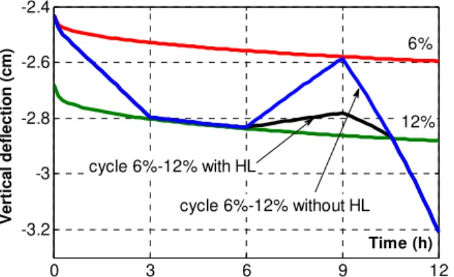
5.2 Example 2: beam in bending and shear In a second example, the beam is loaded by constant transverse loads in four points. The cross-sections are therefore subjected to pure normal stresses in the middle part of the beam, and by a combination of bending normal stresses and shear stresses in the other parts. As a result of the numerical simulation, the vertical deflection at mid-span is presented in figure 5.

(6)

0 3 6 9 12 -3.2 -3 -2.8 -2.6 -2.4 Time (h) V e rt ic a l d e fl e c ti o n ( c m ) 12% 6% cycle 6%-12% with HL cycle 6%-12% without HL

Fig. 5: Effect of varying moisture content on the vertical deflection in constant bending.

As in the previous example, the worked out solutions are compared, with and without hydrolock effect. Here again, the longitudinal deflection (blue line) evolves between the red line (solution for steady ‘dry’ stage) and the green line (solution for steady ‘wet’ stage) in the case when the hydrolock effect is not taken into account. As in the previous case, the hydrolock effect has no effect during the initial moistening phase, while it significantly affects the flexural behavior of the beam during the drying-moistening cycle.

These two computational examples clearly show that the hydrolock effect significantly affects the mechanical response of wooden members when subjected to variable loading and humidity.

6 CONCLUSION

In this paper, the hydrolock effect, previously reported by several authors, was taken into account in a new incremental 3D model of hydromechanical behavior of softwood. The main features of this model are as follows:

- An evolution law is proposed for the hydrolock strain, in accordance with experimental evidences and the principles of thermodynamics.

- The coupling of the hydric, elastic, viscoelastic and hydrolock strain parts is performed, based on the hypothesis of total strain partition.

- The analytical model is turned into an incremental form based on exact integrals. Consequently, the time step is finite, but not necessarily small.

- Taking advantage of the shape of the incremental form, the model can be easily implemented in a FEM software (Cast3m in the present case). The calculation is then worked out as a fictitious equivalent thermoelastic problem. A good accuracy is obtained for low calculation effort.

- The influence of the hydrolock strain was analyzed through two exemplary calculations. The results clearly show that the hydromechanical behavior of wood members is significantly affected by the hydrolock effect, which cannot therefore be omitted in the simulation of wooden structures subjected to variable loading and environmental conditions. 7 ACKNOWLEDGMENTS

This work has been sponsored by the European Regional Development Fund (ERDF) of the European Union, and by the region of Auvergne, France.

8 REFERENCES

[Cariou 1987] Cariou J-L. ; Caractérisation d’un matériau viscoélastique anisotrope : le bois. Doctoral thesis, Bordeaux 1 University, 1987.

[Dubois 2005] Dubois F., Randriambololona H., Petit C.; Creep in wood under variable climate conditions: numerical modeling and experimental validation. Mechanics of Time-Dependent Materials, 2005, vol 9, p.137-202.

[Gril 1988] Gril J.; Une modélisation du comportement hygrorhéologique du bois à partir de sa microstructure. Doctoral thesis, Paris 6 University, 1988.

[Hearmon 1964] Hearmon R.F.S, Paton J.M.; Moisture content changes and creep of wood. Forest Products Journal, 1964, p.357-359.

[Husson 2010] Husson J.M., Dubois F., Sauvat N.; Elastic response in wood under moisture content variations : analytic development. Mechanics of Time-Dependent Materials, 2010, vol 14, p.203-217.

[Saifouni 2014] Saifouni O.; modélisation des effets rhéologiques dans les matériaux: application au comportement mécanosorptif du bois. Doctoral thesis, Blaise Pascal University, Clermont-Ferrand, 2014.