Magnetospheric reconnection driven by solar wind pressure fronts

HAL Id: hal-00317312

https://hal.archives-ouvertes.fr/hal-00317312

Submitted on 2 Apr 2004

HAL is a multi-disciplinary open access

archive for the deposit and dissemination of

sci-entific research documents, whether they are

pub-lished or not. The documents may come from

teaching and research institutions in France or

abroad, or from public or private research centers.

L’archive ouverte pluridisciplinaire HAL, est

destinée au dépôt et à la diffusion de documents

scientifiques de niveau recherche, publiés ou non,

émanant des établissements d’enseignement et de

recherche français ou étrangers, des laboratoires

publics ou privés.

pressure fronts

A. Boudouridis, E. Zesta, L. R. Lyons, P. C. Anderson, D. Lummerzheim

To cite this version:

A. Boudouridis, E. Zesta, L. R. Lyons, P. C. Anderson, D. Lummerzheim. Magnetospheric

reconnec-tion driven by solar wind pressure fronts. Annales Geophysicae, European Geosciences Union, 2004,

22 (4), pp.1367-1378. �hal-00317312�

© European Geosciences Union 2004

Geophysicae

Magnetospheric reconnection driven by solar wind pressure fronts

1_{Department of Atmospheric Sciences, University of California, Los Angeles, USA} 2_{Space Science Applications Laboratory, The Aerospace Corporation, Los Angeles, USA} 3_{Geophysical Institute, University of Alaska, Fairbanks, USA}

Received: 16 April 2003 – Revised: 31 July 2003 – Accepted: 14 November 2003 – Published: 2 April 2004

Abstract. Recent work has shown that solar wind dynamic

pressure changes can have a dramatic effect on the particle precipitation in the high-latitude ionosphere. It has also been noted that the preexisting interplanetary magnetic field (IMF) orientation can significantly affect the resulting changes in the size, location, and intensity of the auroral oval. Here we focus on the effect of pressure pulses on the size of the au-roral oval. We use particle precipitation data from up to four Defense Meteorological Satellite Program (DMSP) space-craft and simultaneous POLAR Ultra-Violet Imager (UVI) images to examine three events of solar wind pressure fronts impacting the magnetosphere under two IMF orientations, IMF strongly southward and IMF Bznearly zero before the

pressure jump. We show that the amount of change in the oval and polar cap sizes and the local time extent of the change depends strongly on IMF conditions prior to the pres-sure enhancement. Under steady southward IMF, a remark-able poleward widening of the oval at all magnetic local times and shrinking of the polar cap are observed after the increase in solar wind pressure. When the IMF Bz is nearly

zero before the pressure pulse, a poleward widening of the oval is observed mostly on the nightside while the dayside remains unchanged. We interpret these differences in terms of enhanced magnetospheric reconnection and convection in-duced by the pressure change. When the IMF is southward for a long time before the pressure jump, open magnetic flux is accumulated in the tail and strong convection exists in the magnetosphere. The compression results in a great enhance-ment of reconnection across the tail which, coupled with an increase of magnetospheric convection, leads to a dramatic poleward expansion of the oval at all MLTs (dayside and nightside). For near-zero IMF Bz before the pulse the open

flux in the tail, available for closing through reconnection, is smaller. This, in combination with the weaker magneto-spheric convection, leads to a more limited poleward expan-sion of the oval, mostly on the nightside.

Key words. Magnetospheric physics (solar

wind-magnetosphere interactions; magnetospheric configuration and dynamics; auroral phenomena)

Correspondence to: A. Boudouridis (thanasis@atmos.ucla.edu)

1 Introduction

The solar wind and the accompanying interplanetary mag-netic field (IMF) are the main drivers of the dynamics of the terrestrial magnetosphere. Solar wind dynamic pressure en-hancements with sufficient duration to engulf the entire mag-netosphere have been shown to induce global responses in short time scales to both ionospheric currents and auroral precipitation (Craven et al., 1986; Shue and Kamide, 1998; Zhou and Tsurutani, 1999; Lyons et al., 2000; Zesta et al., 2000; Chua et al., 2001). Prior work has also shown that the magnetosphere responds very differently to long-duration solar wind pressure changes under different IMF conditions. Elphinstone et al. (1991) studied the auroral signatures dur-ing two pressure pulses that occurred on 19 October 1986 (IMF data discussed by Winglee and Menietti (1998)). A short-lived pressure pulse under northward IMF had only a limited and localized effect on the aurora. A pressure front under southward IMF produced a global and almost imme-diate response of the aurora at all local times. Craven et al. (1986) reported similar results. Specifically, the response to a shock front that hit the magnetosphere under southward IMF conditions was a global intensification of the aurora, occur-ring nearly simultaneously at all MLTs. For a shock that hit under northward IMF conditions there was still a global in-tensification of the aurora at all local times, but it was not as strong as in the southward IMF case. Zesta et al. (2000) found that a pressure enhancement under strong southward IMF triggers an almost instantaneous and global enhance-ment of auroral intensity simultaneously at all local times, a significant widening of the auroral oval, and a closing of the polar cap. Chua et al. (2001) also found a simultane-ous brightening over broad areas of the dayside and night-side aurora in response to a pressure pulse that occurred with a northward turning of the IMF. In some cases, the auro-ral disturbance is clearly observed first at the dayside and then it expands to the nightside (Zhou and Tsurutani, 1999; Boudouridis et al., 2003).

In a recent study, Boudouridis et al. (2003) looked at the effect of solar wind pressure enhancements to the auroral in-tensity, size, and location for three cases with different IMF conditions. They used direct measurements of precipitating

particle fluxes by up to four Defense Meteorological Satel-lite Program (DMSP) spacecraft and simultaneous POLAR Ultra-Violet Imager (UVI) images to investigate the depen-dence of the response of auroral precipitation to an incoming solar wind pressure front on the IMF configuration before and after the front. They concluded that a steady southward IMF throughout the pressure change favors a global intensi-fication of auroral precipitation and ultra-violet (UV) emis-sions, as well as a dramatic (up to 10◦) poleward expansion of the oval at all magnetic local times (MLTs). In the case where the IMF Bz was nearly zero before the pulse, an

in-crease in auroral precipitation was observed all around the oval but now the poleward motion of the high-latitude oval boundary was seen to a lesser degree and only on the night-side, with no apparent motion on the dayside.

In light of these results Boudouridis et al. (2003) raised a fundamental question: “Why does the auroral oval expand poleward after an enhancement of the solar wind dynamic pressure, and why is this response different for different pre-existing IMF configurations?” Boudouridis et al. (2003) suggested that the sudden poleward expansion of the oval away from the noon MLT sector after the arrival of a solar wind pressure front was associated with enhanced tail recon-nection triggered by the compression of the magnetosphere. Open field lines close at a higher rate as the open-closed field line boundary (OCB) and thus, the poleward boundary of the auroral oval moves toward higher latitudes. The observations show that the shrinking of the polar cap is more extensive and over a broader MLT range in the case of southward IMF conditions prior to the pressure front impact. Therefore, the strength of the enhanced tail reconnection and its local time variation are dependent on the previous state of the magne-tosphere (preconditioning), which, in turn, depends on the preexisting IMF structure. We believe that the surprising re-sult of a poleward motion in the noon sector must also be related to increased reconnection, but how the reconnection process can result in more closed field lines on the dayside is unclear.

In the following sections we discuss observations of the shrinking polar cap (as seen by DMSP particle detectors and POLAR UVI images) and examine how nightside reconnec-tion leads to different results under two different IMF config-urations: a) IMF steady southward throughout the pressure pulse event and b) IMF Bz nearly zero before the pressure

increase. We are able to show that even though the sharp large-scale compression causes enhancement of magnetotail reconnection under both IMF configurations, higher avail-able open flux near the nightside separatrix and much higher convection under southward IMF Bz (i.e. preconditioning)

are associated with the more spectacular and global changes in the auroral oval under those IMF conditions (both dayside and nightside) compared with the IMF Bz≈0 case (nightside

only). In Sect. 2 we describe the effects of a pressure front on the auroral oval and polar cap sizes. In Sect. 3 we discuss the role of magnetospheric reconnection in the different re-sponses observed under different IMF conditions. Finally, in Sect. 4 we summarize our conclusions.

2 Effects of pressure fronts on aurora

We examine three case studies occuring under the above IMF conditions. The first one on 10 January 1997 is a pressure pulse event under steady southward IMF. Its auroral response to the pressure pulse has been studied by many authors in the past (e.g. Lyons, 2000; Lyons et al., 2000; Zesta et al., 2000; Boudouridis et al., 2003). Here we give a summary of the previous results on this event which we then compare with the new results for the IMF Bz≈0 case presented in Sect. 2.2.

The other two events, on 6 January and 30 April 1998, take place under near-zero IMF Bzconditions prior to the pressure

front impact.

2.1 IMF Bz<0

During the widely studied storm of 10 January 1997, a sig-nificant and abrupt pressure increase was recorded by the WIND spacecraft at ∼10:30 UT, lasted ∼22 min and reached the Earth at ∼10:50 UT. Its duration, combined with a solar wind velocity of 450 km/sec, yields a radial size of ∼93 RE

for the high-pressure region in the solar wind, the pressure in it being three times higher than that recorded before and after. This is large enough to engulf and compress the en-tire magnetosphere. During this event the IMF Bzremained

strongly negative at all times, following a long period (from 05:00 UT onwards) of strongly southward IMF (Lyons et al., 2000). Therefore, it is an ideal event for studying the effect of a solar wind dynamic pressure enhancement on the size of the polar cap under southward IMF conditions.

Lyons et al. (2000) and Zesta et al. (2000) looked at the effect of the above pressure enhancement on the auro-ral emissions measured by meridional scanning photome-ters (MSPs) from the CANOPUS stations at Rankin Inlet and Gillam. They found that the poleward boundary of the 6300 ˚A and 5577 ˚A emissions tracks the solar wind density and pressure, moving poleward in response to pressure en-hancements, while the emission levels are enhanced during the high pressure interval. Zesta et al. (2000) and Lyons (2000) presented POLAR UVI measurements of the North-ern Hemisphere nightside polar region during the period of the above pressure pulse. They showed a significant increase in auroral emissions at around 10:50 UT, accompanied by a poleward motion of the high-latitude auroral boundary (up to 10◦_{at some MLTs) and a widening of the auroral oval at}

all visible MLTs. The UV emissions dropped to their pre-pulse levels at around 11:20 UT, coincident with the solar wind pressure drop. Variations in the auroral emissions were, therefore, directly driven by the solar wind dynamic pressure changes.

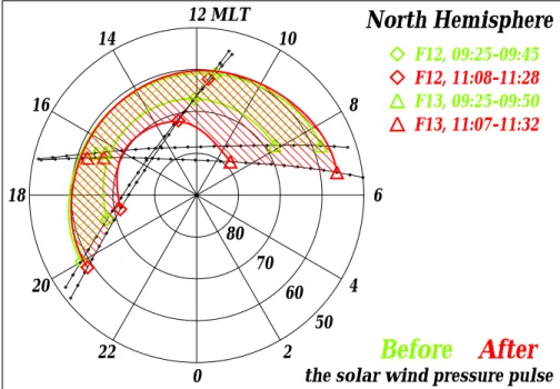
Boudouridis et al. (2003) studied the same event, this time using directly measured DMSP precipitating particle fluxes from two spacecraft, F12 and F13. They looked for changes in the size and intensity of the auroral oval caused by the incoming pressure pulse. Figure 1 shows the auro-ral boundaries before (green) and after (red) the increase in solar wind pressure at 10:50 UT. The individual boundary

50

60

70

80

0

2

4

6

8

10

12

14

16

18

20

22

MLT

_{North Hemisphere}

F12, 09:25-09:45

F12, 11:08-11:28

F13, 09:25-09:50

F13, 11:07-11:32

Before

After

the solar wind pressure pulse

Fig. 1. Auroral boundaries for 10 January 1997, based on the individual boundary identifications from the DMSP spectrograms. The satellite

orbits are shown as black lines. The tick marks on them are one minute apart. The big diamonds and triangles represent the actual boundary determinations for F12 and F13, respectively. The green and red curves are the inferred oval boundaries for before and after the arrival of the solar wind pressure front (Boudouridis et al., 2003). A closing of the polar cap is observed at all MLTs.

determinations were based mainly on 2 keV electron dif-ferential energy fluxes, as described in Boudouridis et al. (2003), and are marked by the big diamonds and triangles for F12 and F13, respectively. The green and red curves are the oval boundaries before and after the arrival of the solar wind pressure front, derived by a simple spline fit on the ac-tual boundary crossings which was then smoothed to pro-duce a more continuous boundary. The high-latitude bound-ary moves clearly poleward in the region of ∼8–20 MLT af-ter the pressure jump. This motion is a few degrees in the dusk region and as much as 10◦ in the dawn region. Fur-thermore, Boudouridis et al. (2003) showed that the total en-ergy input into the ionosphere due to particle precipitation greatly increased after the pressure pulse impact, covering a substantially wider auroral oval, with fluxes of the order of 1011–1012 eV/(cm2ster sec).

The simultaneous widening of the oval and shrinkage of the polar cap on both the dayside (DMSP data, (Boudouridis et al., 2003)) and the nightside (UV data, (Lyons, 2000; Zesta et al., 2000)) signifies a global response of the magnetosphere-ionosphere system to the incoming pressure pulse. This response is energetically very important and, as we show later on, closely associated with the preexisting state of the magnetosphere.

2.2 IMF Bz≈0 before the pressure change

Boudouridis et al. (2003) also studied an event on 2 Octo-ber 1998, where the IMF Bz was close to zero before the

pressure increase and substantially fluctuated after. Their

main conclusion was that the auroral precipitation response in this case was not as strong as in the southward-IMF 10 Jan-uary 1997 case. The dayside oval did not show a significant change in its size but the auroral UV emissions did increase after the pressure shock, with the emissions’ intensification exhibiting a small noon-to-midnight propagation, especially in the Northern Hemisphere duskside. On the nightside, there was a substantial poleward widening of the oval and increased particle precipitation, seen in both the DMSP and Polar UV observations. However, the closing of the polar cap on the nightside was again less dramatic compared with the southward-IMF 10 January 1997 event.

The nightside intensification and poleward motion resem-bles the effects of a substorm. However, the auroral observa-tions as well as geosynchronous energetic particle data (e.g. Fig. 14 of Boudouridis et al. (2003)), clearly showed that the general response is not due to substorms. In particular, the ef-fects of the pressure fronts occur over a wide range of MLTs as opposed to the more localized (premidnight) substorm fea-tures. Also, ionospheric currents show an enhancement in the large-scale DP2 current, and do not show the nightside en-hancement of the westward electrojet that is associated with the substorm current wedge (Zesta et al., 2000).

In order to better understand the behavior of the auroral oval in this near-zero preceding IMF Bz scenario and test

the generality of the results obtained for the 2 October 1998 event, we examine two more events of this kind.

10 11 12 13 14 15 16 17 18 Universal Time (hours)

-10 -5 0 5 10 Bz (nT) ACE 10 11 12 13 14 15 16 17 18 -10 -5 0 5 10 Bz (nT) IMP8 10 11 12 13 14 15 16 17 18 -10 -5 0 5 10 Bz (nT) WIND 10 11 12 13 14 15 16 17 18 2 4 6 8 10 Psw (nPa) IMP8 10 11 12 13 14 15 16 17 18 2 4 6 8 10 Psw (nPa) WIND

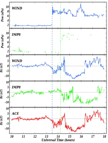
Fig. 2. Solar wind conditions for 6 January 1998. The top two

panels show the solar wind dynamic pressure observed by WIND

and IMP8, while the three bottom panels show the IMF Bz

com-ponent in GSE coordinates measured by WIND, IMP8, and ACE.

The three spacecraft were located at X_GSE∼227R_E, X_GSE∼30R_E,

and XGSE∼220 RE, for WIND, IMP8, and ACE, respectively. The

vertical lines mark the times when WIND (blue) and IMP8 (green) encountered the pressure front. The pressure front impacted the magnetosphere at ∼14:25 UT.

2.2.1 Event 1: 6 January 1998

Figure 2 shows solar wind pressure and IMF Bz

mea-surements for the pressure increase on 6 January 1998 at ∼14:25 UT. The top two panels show the solar wind dynamic pressure observed by WIND and IMP8, while the three bot-tom panels show the IMF Bzcomponent in GSE coordinates

measured by WIND, IMP8, and ACE. The solar wind pres-sure front was first detected by WIND at ∼13:30 UT. The dy-namic pressure exhibited a step change from 2 nPa to ∼8 nPa and then remained high at ∼8 nPa for many hours. The im-pact at the magnetosphere was estimated to be at ∼14:20– 14:25 UT consistent with the IMP8 detection of the pressure front at ∼14:15 UT at XGSE∼30 RE. The IMF Bzpreceding

this pressure front was almost zero for many hours before, and at impact it turned negative and remained mostly nega-tive until ∼17:25 UT. There was only a short-lived northward turning at ∼15:20 UT.

The polar maps of the DMSP boundary identifications (based on three DMSP spacecraft) for this event are shown in

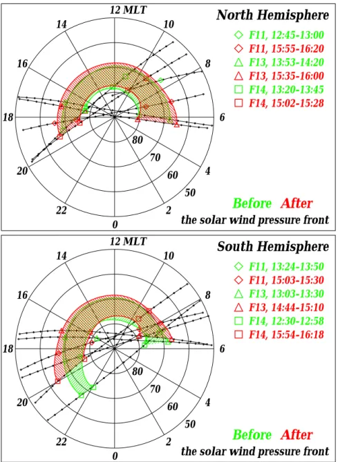
Fig. 3. The format of this plot is the same as in Fig. 1, with the Northern Hemisphere passes shown on the top and South-ern Hemisphere passes shown on the bottom panel. Figure 3 indicates that the size and location of the dayside auroral oval remained unchanged for both hemispheres from before (green) to after (red) the solar wind pressure change. Notice that the poleward boundary of the oval before the pressure enhancement was already at high latitude (∼78◦) as com-pared with the same boundary for the 10 January 1997 case (at ∼68◦).

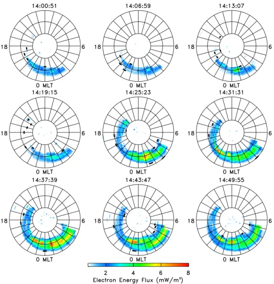
The nightside sector is better seen in the POLAR UVI data shown in Fig. 4 for the Northern Hemisphere. Nine im-ages of derived electron energy flux are shown, one every ∼6 min, from ∼14:01 UT (top left) until ∼14:50 UT (bot-tom right). The three circles in each image correspond to magnetic latitudes of 60◦_{, 70}◦_{, and 80}◦_{. An intensification}

is clearly observed at all available MLTs (within the field of view of POLAR at that time) at ∼14:25 UT (5th image), with intensity increasing from ∼3 to ∼7 mW/m2in the postmid-night region. A poleward expansion of the oval begins at the same time on the nightside, reaching ∼75◦of latitude at ∼14:44 UT. It is important to point out here that the closing of the polar cap on the nightside occurs at the same time as the IMF Bz turns negative, which would normally open the

polar cap. However, for this event the effects of the pressure enhancement (i.e. closing of the polar cap) counteract the ef-fects of the IMF southward turning.

2.2.2 Event 2: 30 April 1998

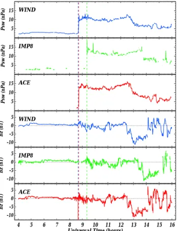
For the second event we concentrate on the period 04:00– 16:00 UT on 30 April 1998. The IMF Bz and solar wind

dynamic pressure data for this period are shown in Fig. 5. The top three panels show the solar wind dynamic pressure observed by WIND, IMP8, and ACE, while the three bot-tom panels show the IMF Bzcomponent in GSE coordinates

measured by the same spacecraft. All three spacecraft record a remarkably similar behavior of both the dynamic pressure and the IMF Bz component. The pressure, being quite low

for many hours prior to the front (∼2–3 nPa), jumps to a 12– 14 nPa value and remains at this high level for about 4 h. The IMF Bz, on the other hand, stays more or less stable at

near-zero values throughout the pressure change, exhibiting only a slightly higher degree of variability under the high pres-sure. The arrival time of the front at the nose of the magne-tosphere is estimated at ∼09:25 UT, in agreement with the IMP8 crossing at ∼09:20 UT. This event is ideally suited for examining the effects of solar wind dynamic pressure enhancements under IMF Bz≈0 conditions throughout the

pressure change.

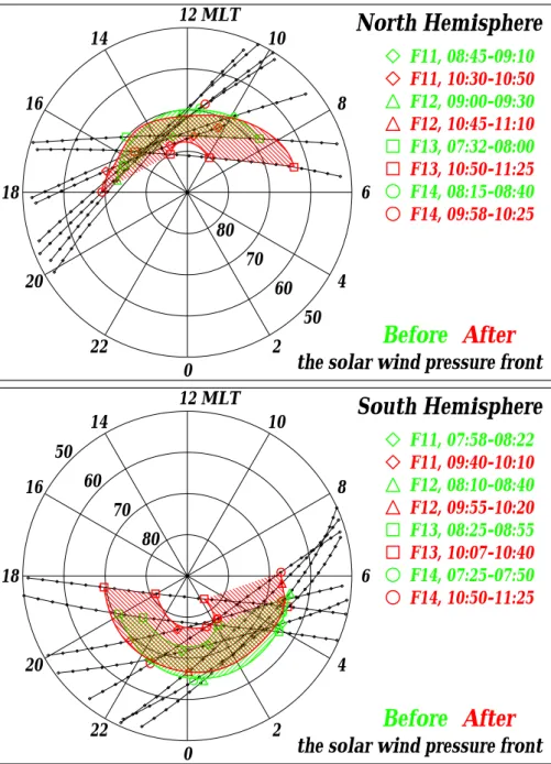
The oval location based on the DMSP particle characteris-tics is shown in Fig. 6 in the same format as in Fig. 3. In the Northern Hemisphere (top), no satellite crosses the poleward boundary of the dayside oval (green shading) before the pres-sure increase. The highest latitude reached (by F11) is ∼76◦, and thus, the boundary lies poleward of that latitude. After the front impact, the poleward boundary is detected by F11

50 60 70 80 0 2 4 6 8 10 12 14 16 18 20 22 MLT

_{North Hemisphere}

Before

After

the solar wind pressure front

50 60 70 80 0 2 4 6 8 10 12 14 16 18 20 22 MLT

_{South Hemisphere}

Before

After

the solar wind pressure front

Fig. 3. The same as in Fig. 1 for 6 January 1998, North Hemisphere on the top and South Hemispere on the bottom. The various symbols

denoting the boundary crossings by different spacecraft are explained at the legend on the right. No poleward motion of the dayside oval is observed.

at around the same latitude, and by F13 at 80◦. Therefore, it is uncertain if any poleward motion took place at the day-side due to the pressure enhancement. However, conday-sidering again the very high starting point of the poleward boundary (>76◦ before the pulse), there was most likely no signifi-cant closing of the polar cap at the dayside. In the South-ern Hemisphere (bottom panel) the situation is very differ-ent. The nightside oval responds to the change in solar wind pressure by expanding poleward by about 5◦_{, as observed by}

the F11 and F13 spacecraft which crossed the high-latitude oval boundary both before and after the high pressure im-pact. Since the oval’s equatorward boundary remains more or less stationary, the result is a significant increase in the oval width.

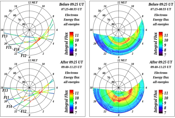
There are no UV images for this event, but the change in the southern nightside oval size, together with an increase in auroral particle precipitation, are clearly demonstrated in the electron integral flux plots of Fig. 7. The two panels on the left depict, as a color-coded trace, the electron integral energy flux measured along the DMSP orbits before (top) and after (bottom) the increase in solar wind dynamic pressure. The panels on the right show simple two-dimensional interpola-tions of the trace fluxes. Both display formats show a much wider oval with intensity about an order of magnitude higher in most locations in the “after” panels (bottom) as compared with the “before” panels (top).

Fig. 4. POLAR UVI measurements for 6 January 1998. Nine images of derived electron energy flux are shown, one every ∼6 min, starting

at ∼14:01 UT (top left) until ∼14:50 UT (bottom right). An intensification is observed at all available MLTs at ∼14:25 UT (5th image), and a poleward expansion of the oval is observed on the nightside. The absence of dayside UV emissions in this plot is due to the limited field of view of the POLAR spacecraft. An enhancement of auroral precipitation was indeed observed in the dayside oval by the DMSP spacecraft.

3 The role of magnetospheric reconnection

As mentioned in the Introduction, an important question arises now (Boudouridis et al., 2003): “What causes the auro-ral oval to expand poleward and the polar cap size to dimin-ish in response to the compression of the magnetosphere?” Boudouridis et al. (2003) briefly discussed the various pos-sibilities and concluded that the large and rapid shrinking of the polar cap that occurs in response to dynamic pressure en-hancements corresponds to a large and rapid decrease in the amount of open polar cap magnetic flux. Such a conversion of open to closed flux must be a manifestation of reconnec-tion. But why is the response different under different preex-isting IMF conditions? What leads to the tremendous pole-ward widening of the oval at all MLTs in the southpole-ward IMF case as opposed to the more limited nightside motion in the near-zero Bzcase?

We argue that most of the polar cap shrinkage is associated with increased nightside reconnection, and that the strength and MLT extent of this enhanced magnetotail reconnection depends on the previous state of the magnetosphere. A sum-mary of our observations and current understanding of how this works under different preexisting IMF orientations to produce the observed polar cap shrinkage, is given in the schematic representation of the polar region in Fig. 8. The top panel describes the auroral response when IMF Bz<0 and

the bottom panel describes the situation when IMF Bz≈0

be-fore the front impact. The blue solid lines mark the location of the poleward boundary of the oval before the pressure in-crease, and the red ones mark the position of the same bound-ary as observed after the pressure jump. The solid green line denotes the poleward boundary of the region where field lines that map to the tail, close as a result of the pressure enhance-ment. This simple drawing does not include the effects of an IMF Bycomponent that would distort the regions drawn

4 5 6 7 8 9 10 11 12 13 14 15 16 Universal Time (hours)

-10 -5 0 5 Bz (nT) ACE 4 5 6 7 8 9 10 11 12 13 14 15 16 -10 -5 0 5 Bz (nT) IMP8 4 5 6 7 8 9 10 11 12 13 14 15 16 -10 -5 0 5 Bz (nT) WIND 4 5 6 7 8 9 10 11 12 13 14 15 16 5 10 15 Psw (nPa) ACE 4 5 6 7 8 9 10 11 12 13 14 15 16 5 10 15 Psw (nPa) IMP8 4 5 6 7 8 9 10 11 12 13 14 15 16 5 10 15 Psw (nPa) WIND

Fig. 5. Solar wind conditions for 30 April 1998. The top three

panels show the solar wind dynamic pressure observed by WIND, IMP8, and ACE, while the three bottom panels show the IMF

Bz component in GSE coordinates measured by the same

space-craft. WIND, IMP8, and ACE were located at X_GSE∼217 R_E,

XGSE∼27 RE, and XGSE∼229 RE, respectively. The vertical lines

mark the detection times of the front by the three spacecraft. The high pressure front impacted the magnetosphere at ∼09:25 UT.

In the first case (top), the strong negative IMF Bz(present

for a long period before the pulse) has acted to open the polar cap wide (blue line), resulting in a large region of open field lines mapping back into the tail (green hatched area). When the pressure front impacts the magnetosphere, enhanced reconnection in the tail closes these open field lines as the OCB moves poleward. This area occupies not only the nightside portion of the polar cap, but also extends along the dawn/dusk flanks. This produces much of the global re-sponse seen in cases like 10 January 1997. However, this cannot account for the dayside polar cap closing near noon (red hatched area) observed in this event.

In the Bz≈0 case (bottom panel) the polar cap is already

considerably closed before the arrival of the pressure front (the dashed blue line is the location of the poleward oval boundary for IMF Bz<0, shown for comparison). The tail

field lines below the solid blue line have already been closed due to the prolonged near-zero IMF Bz. Therefore, when

the pressure front hits the magnetosphere, enhanced tail re-connection closes only a smaller portion of open tail field

lines (green hatched area in bottom panel) compared with the southward IMF case. This results in a diminished observable response of the size and location of the auroral oval, limited mostly to the nightside. The dayside oval does not show any size or location variation, as was seen for the 6 January and 30 April 1998 events.

Additional information on the different responses for the two IMF cases can be obtained by using the Tsyganenko-96 (hereinafter referred to as TTsyganenko-96) geomagnetic field model (Tsyganenko, 1995, 1996). Despite the limitations of this model in determining the separatrix between the open and closed field lines in the tail, qualitative results can be de-rived showing the difference in the magnetospheric configu-ration before a pressure front impact for the two IMF condi-tions, that leads through enhanced magnetotail reconnection to the different ionospheric responses observed by the DMSP spacecraft.

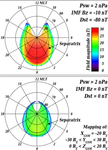
Figure 9 shows results of T96 field line tracing for the con-ditions present right before the solar wind pressure enhance-ment (Psw=2 nPa). It depicts how the field magnitude and

lo-cation in the magnetotail region defined by XGSM=−20 RE,

−30 RE<YGSM<30 RE, 0 RE<ZGSM<20 RE, map down to

the source of the field lines in the high-latitude ionosphere for the two IMF conditions preceding the pressure front ar-rival, strongly southward IMF (top) and near-zero IMF Bz

(bottom). The dipole tilt and the IMF By component were

assumed to be zero in this simulation, to guarantee north-south and dawn-dusk symmetry of the results. The color-coded images represent the total field magnitude in the tail, expressed in nT , according to the color scale at the right. The solid black line gives the approximate location of the separatrix. This was determined by tracing the field lines to the last point, near 100 RE downtail, and checking to see if

they crossed the equatorial plane (ZGSM=0). All field lines

that reached 100 RE downtail without crossing the

equato-rial plane were defined as open. Obviously, this criterion is not entirely accurate as some field lines might close fur-ther downtail, moving the actual position of the separatrix to higher ZGSM.

However, the uncertainty in the exact location of the sep-aratrix does not affect our qualitative conclusions here. The difference in the field strength in the tail for the two cases is what really matters. In the top panel the field is accumulated in the tail as a result of the negative IMF Bz. This region of

high tail field strength maps to the polar cap area in which the rapid and widespread poleward widening of the oval is observed by the DMSP satellites. Our observations show that, under these conditions, a compression of the magneto-sphere is related to reconnection along the separatrix region all across the tail. The enhanced tail magnetic field could be the reason why tail reconnection is more efficient in closing open magnetic flux over a wide range of MLTs for the south-ward IMF case. The same polar cap area in the near-zero Bz

case maps to a tail region with 30% lower field magnitude. The total magnetic flux in the near-separatrix region, for ex-ample, in a strip 3 REabove the separatrix, is 24% lower in

50

60

70

80

0

2

4

6

8

10

12

14

16

18

20

22

MLT

_{North Hemisphere}

F11, 08:45-09:10

F11, 10:30-10:50

F12, 09:00-09:30

F12, 10:45-11:10

F13, 07:32-08:00

F13, 10:50-11:25

F14, 08:15-08:40

F14, 09:58-10:25

Before

After

the solar wind pressure front

50

60

70

80

0

2

4

6

8

10

12

14

16

18

20

22

MLT

_{South Hemisphere}

F11, 07:58-08:22

F11, 09:40-10:10

F12, 08:10-08:40

F12, 09:55-10:20

F13, 08:25-08:55

F13, 10:07-10:40

F14, 07:25-07:50

F14, 10:50-11:25

Before

After

the solar wind pressure front

Fig. 6. The same as in Fig. 3 for 30 April 1998, North Hemisphere on the top and South Hemispere on the bottom. The various symbols

denoting the boundary crossings by different spacecraft are explained at the legend on the right. A significant poleward expansion of the nightside South Hemispere oval is observed.

this configuration closes the polar cap on the nightside where the tail field strength is still high, but not on the flanks where the tail field strength is weaker.

Enhanced magnetotail reconnection can explain the po-lar cap shrinkage observed in the IMF Bz≈0 cases. But

it still cannot fully explain the southward IMF case. The closing of the polar cap in the 8–16 MLT range sug-gests the contribution of another process that “closes” field lines on the dayside. There is a possible con-nection to the enhanced magnetotail reconcon-nection which is opposite from what is normally expected for IMF Bz<0. If the increased reconnection in the tail is

cou-pled with enhanced magnetospheric convection induced by the pulse, then it is possible to transport the newly-closed tail/flank field lines to the dayside in much shorter time scales than usual.

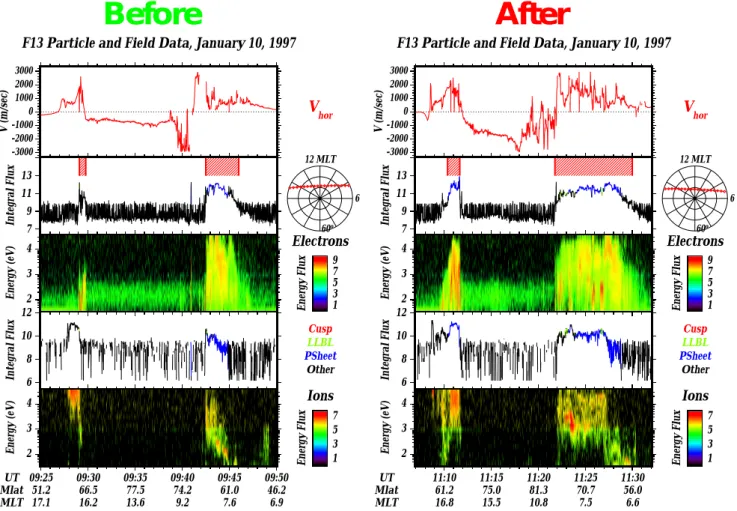
Evidence of enhanced ionospheric convection can be found during the 10 January 1997 event in the DMSP elec-tric field data and the associated ionospheric flows. Figure 10 shows data from two DMSP F13 passes, before (left) and af-ter (right) the pressure pulse event. Each plot shows (from top to bottom) ionospheric horizontal velocity, electron inte-gral energy flux, electron differential energy flux, ion inteinte-gral energy flux, and ion differential energy flux. The spacecraft

50 60 70 80 0 2 4 6 8 10 12 14 16 18 20 22 MLT F11 F12 F13 F14

Integral Flux

₇

8

9

10

11

Integral Flux

₇

8

9

10

11

Integral Flux

₇

8

9

10

11

Integral Flux

₇

8

9

10

11

Fig. 7. DMSP electron integral energy fluxes for the Southern Hemisphere on 30 April 1998. The two panels on the left are the actual

measurements before (top) and after (bottom) the solar wind pressure front. The panels on the right are two-dimensional interpolations of the trace fluxes on the left. An intensification and poleward expansion of the aurora are clearly observed.

orbit is shown in the inset to the right of the electron inte-gral energy flux. The auroral oval crossings for these passes are marked by the hatched boxes above the electron integral energy flux curves, and correspond to the regions marked by the triangles along the F13 orbits in Fig. 1. The iono-spheric velocity is measured in the direction perpendicular to the spacecraft orbit, which in this case is almost along the noon-midnight direction. Positive velocities are sun-ward and negative velocities are antisunsun-ward. The “after” pass shows dramatically enhanced flows all along the satel-lite orbit. Inside the dawn oval, which expanded poleward by ∼10◦, the ionospheric velocity increased from ∼600 m/s to ∼1500–2000 m/s. This high convection velocity can trans-port a newly-closed field line along the 70◦ latitude circle from the flanks (∼5 MLT) to noon in about 30 min, and in even shorter times for higher latitudes. F13 crossed the ex-panded poleward oval boundary after the pressure front at 11:22 UT, ∼32 min after the front impact at ∼10:50 UT.

Therefore it is possible that increased convection in the magnetosphere can move the newly-reconnected field lines piling up at the nightside and flanks to the dayside after the pressure front impact. When this convection is as high as in the southward IMF case, a large amount of closed flux can

be transported rapidly to the dayside, producing the closing of the polar cap observed there for this case. Enhanced iono-spheric convection has also been observed for the IMF Bz≈0

cases, but of considerably smaller magnitude which renders it unable to transfer newly-closed flux from the tail to the dayside in short time scales.

Finally, we would like to comment briefly on how the IMF orientation after the pressure change affects the above auro-ral response. Boudouridis et al. (2003) showed an event on 18 February 1999, where the IMF was strongly negative be-fore and it turned strongly positive after the increase in solar wind pressure. According to the above interpretation for the IMF Bz<0 case, we again expect to see closing of the

po-lar cap. And this was actually observed on the dayside. The difference now is that the northward turning of the IMF can also result in the closing of the polar cap and the two effects are not easily distinguishable. The poleward widening of the oval in this case was detected by the DMSP F12 spacecraft 48 min after the simultaneous front impact and IMF north-ward turning. This time is long enough for the reconfig-uration of the polar cap convection due to changes in IMF orientation, ∼12–24 min (Ridley et al., 1997), and the clos-ing of the polar cap due to the pressure pulse, ∼10–15 min

0 2 4 6 8 10 12 14 16 18 20 22 MLT 60 70 80

IMF Bz < 0

0 2 4 6 8 10 12 14 16 18 20 22 MLT 60 70 80

IMF Bz = 0

Fig. 8. A diagram illustrating the role of enhanced magnetotail

re-connection in closing the polar cap after the arrival of the pressure

front, for IMF Bz<0 (top) and IMF Bz≈0 (bottom). The green

hatched area in both panels represents the area of previously open tail field lines now closing due to the pressure enhancement. This mechanism, however, cannot account for the dayside polar cap

clos-ing when IMF Bz<0 (red hatched area on the top panel).

(Zesta et al., 2000), to take place. Most likely, both effects contributed to the closing of the polar cap in this case. In ad-dition, a simultaneous substorm developed on the nightside and obscured the effects of the pressure change there. The two events under near-zero preceding IMF Bz that we

stud-ied here (Sect. 2.2) have a different IMF Bzorientation after

the pressure jump, one turns southward and the other remains zero, but this does not produce any observable differences in the DMSP or POLAR UVI responses.

4 Conclusions

We can summarize our observations as follows. When the IMF is strongly southward before the increase in solar wind dynamic pressure, the oval responds most spectacularly to the impacting front. A poleward expansion of the oval is witnessed at all MLTs, more or less simultaneously, ranging from a few degrees to up to 10◦ at some longitudes. This tremendous increase in the oval size and the ensuing shrink-ing of the polar cap area are accompanied by an enhancement

0 2 4 6 8 10 12 14 16 18 20 22 MLT Separatrix 60 70 80

Psw = 2 nPa

IMF Bz = -10 nT

Dst = -80 nT

Psw = 2 nPa

IMF Bz = 0 nT

Dst = 0 nT

Fig. 9. Results of the Tsyganenko-96 geomagnetic field model for

the two IMF cases prior to the pressure enhancement (Psw=2 nPa),

IMF strongly southward (top), and IMF Bz=0 (bottom). The

color-coded images represent the mapping to the ionosphere of the total

field magnitude in the tail (XGSM=−20 RE), expressed in nT

ac-cording to the color scale at the right. The solid black line gives the approximate location of the separatrix. The field strength in the top panel is 30% higher than that in the bottom panel, resulting in a more efficient reconnection enhancement after the pressure front impact, that leads to a more widespread shrinking of the polar cap.

of the precipitating particles energy input in the ionosphere all around the oval. This is a global response, characteristi-cally different from the more localized effects of substorms (e.g. Boudouridis et al., 2003). When IMF Bz≈0 before the

pressure front impact, the auroral precipitation reacts differ-ently than when IMF Bz<0. An intensification of the oval

occurs again at all MLTs, but in this case a poleward expan-sion of the oval takes place predominantly on the nightside, whereas the dayside oval seems unchanged in size and loca-tion.

These observations strongly support the idea that pre-conditioning plays an important role in the response of the magnetosphere to the incoming solar wind pressure fronts. Specifically, we associate the closing of the polar cap with an enhancement of magnetotail reconnection resulting from the compression of the magnetosphere by the high-pressure solar wind, because the reduction of open polar cap flux observed

Before

After

F13 Particle and Field Data, January 10, 1997

Energy Flux 1 3 5 7 9 2 3 4 Energy (eV) 7 9 11 13 Integral Flux Electrons Energy Flux 1 3 5 7 09:25 09:30 09:35 09:40 09:45 09:50 51.2 66.5 77.5 74.2 61.0 46.2 17.1 16.2 13.6 9.2 7.6 6.9 2 3 4 UT Mlat MLT Energy (eV) 6 8 10 12 Integral Flux Ions Cusp LLBL PSheet Other 12 MLT 6 60o -3000 -2000 -1000 0 1000 2000 3000 V (m/sec) V_hor

F13 Particle and Field Data, January 10, 1997

Energy Flux 1 3 5 7 9 2 3 4 Energy (eV) 7 9 11 13 Integral Flux Electrons Energy Flux 1 3 5 7 11:10 11:15 11:20 11:25 11:30 61.2 75.0 81.3 70.7 56.0 16.8 15.5 10.8 7.5 6.6 2 3 4 UT Mlat MLT Energy (eV) 6 8 10 12 Integral Flux Ions Cusp LLBL PSheet Other 12 MLT 6 60o -3000 -2000 -1000 0 1000 2000 3000 V (m/sec) V_hor

Fig. 10. DMSP F13 particle and electric field data for 10 January 1997, before (left) and after (right) the pressure pulse event. Each plot shows

(from top to bottom) horizontal ionospheric velocity, electron integral energy flux, electron differential energy flux, ion integral energy flux, ion differential energy flux. The spacecraft orbit is shown in the inset to the right of the electron integral energy flux. The red hatched boxes above the electron integral flux curves denote the oval locations as determined in Fig. 1. The ionospheric velocity is measured perpendicular to the spacecraft orbit, in this case almost along the day-night direction, sunward when positive and antisunward when negative. Dramatically enhanced flows all along the satellite path are seen in the “after” pass.

requires a significant closing of field lines. Furthermore, we suggest that the magnitude and local time variation of this reconnection enhancement are controlled by the IMF orien-tation prior to the arrival of the pressure front.

When the IMF is southward for a long time before the pressure jump, the polar cap is wide open, the magnetotail is loaded with energy (open, stretched field lines, closely packed together), and in general, the magnetosphere is very “receptive” to a sudden change in solar wind pressure. The result is a great enhancement of reconnection across the tail, which, coupled with an increase of magnetospheric convec-tion, leads to a dramatic poleward expansion of the oval and shrinking of the polar cap at all MLTs. On the other hand, when IMF Bzis almost zero before the pulse, the

mag-netic flux of open field lines in the tail, available for closing through reconnection, is smaller. This, in combination with the weaker enhancement of ionospheric convection due to the pressure change, results in a more limited poleward ex-pansion of the oval, mostly on the nightside.

In conclusion, we can reliably say that the preexisting IMF structure affects the ability of the magnetosphere to respond to the incoming pressure change. On the other hand, the IMF conditions following the pressure enhancement are important in our ability to clearly observe and isolate this response from other concurrent processes. More events need to be studied, encompassing the full spectrum of IMF orientation before and after the pressure front impact. Also, the above conclu-sion of enhanced magnetotail reconnection as a response to an increase in solar wind pressure, could be further inves-tigated by looking for signatures of enhanced reconnection and convection, both at low altitudes (e.g. DMSP data) and locally in the tail (e.g. Geotail data).

Acknowledgements. The authors wish to acknowledge N. Ness at

Bartol Research Institute, A. Szabo and R. P. Lepping at NASA GSFC, D. J. McComas at LANL, A. Lazarus at MIT, K. Ogilvie at NASA GSFC, and CDAWeb for the use of IMF and plasma data from the ACE, IMP8, and WIND spacecraft. This work was sup-ported by NASA grant NAG5-12007 and NSF grant OPP-0136139. P. C. Anderson acknowledges support from NSF grant

NSF-ATM-0000268. Topical Editor T. Pulkkinen thanks K. Nykiri and

another referee for their help in evaluating this paper.

References

Boudouridis, A.: Zesta, E., Lyons, L. R., Anderson, P. C., and Lum-merzheim, D.: Effect of solar wind pressure pulses on the size and strength of the auroral oval, J. Geophys. Res., 108(A4), 8012, doi:10.1029/2002JA009373, 2003.

Chua, D., Parks, G., Brittnacher, M., Germany, G., and Spann, J.: Energy characteristics of auroral electron precipitation: A com-parison of substorms and pressure pulse related auroral activity, J. Geophys. Res., 106, 5945–5956, 2001.

Craven, J. D., Frank, L. A., Russell, C. T., Smith, E. J., and Lepping, R. P.: Global auroral responses to magnetospheric compressions by shocks in the solar wind: Two case studies, in: Solar Wind-Magnetosphere Coupling, edited by Kamide, Y., and Slavin, J. A., 367–380, Terra Scientific, Tokyo, 1986.

Elphinstone, R. D., Murphree, J. S., Cogger, L. L., Hearn, D., and Henderson, M. G.: Observations of changes to the auroral distri-bution prior to substorm onset, in: Magnetospheric Substorms, Geophys. Monogr. Ser., vol. 64, edited by Kan, J., Potemra, T. A., Kokubun, S., and Iijima, T., 257, AGU, Washington, D. C., 1991.

Lyons, L. R.: Geomagnetic disturbances: characteristics of, distinc-tion between types, and reladistinc-tions to interplanetary condidistinc-tions, J. Atmos. Solar-Terr. Phys., 62, 1087–1114, 2000.

Lyons, L. R., Zesta, E., Samson, J. C., and Reeves, G. D.: Auroral disturbances during the January 10, 1997 magnetic storm, Geo-phys. Res. Lett., 27, 3237–3240, 2000.

Ridley, A. J., Gang, L., Clauer, C. R., and Papitashvili, V. O.: Ionospheric convection during nonsteady interplanetary mag-netic field conditions, J. Geophys. Res., 102, 14,563–14,579, 1997.

Shue, J.-H. and Kamide, Y.: Effects of solar wind density on the westward electrojet, in: SUBSTORMS-4, edited by Kokubun, S. and Kamide, Y., 677–680, 1998.

Tsyganenko, N. A.: Modeling the Earth’s magnetospheric magnetic field confined within a realistic magnetopause, J. Geophys. Res., 100, 5599–5612, 1995.

Tsyganenko, N. A.: Effects of the solar wind conditions on the global magnetospheric configuration as deduced from data-based field models, in Proceedings of the ICS-3 Conference on Sub-storms, Eur. Space Agency Spec. Publ., vol. 389, 181–185, 1996. Winglee, R. M. and Menietti J. D.: Auroral activity associated with pressure pulses and substorms: A comparison between global fluid modeling and Viking UV imaging, J. Geophys. Res., 103, 9189–9205, 1998.

Zesta, E., Singer, H. J., Lummerzheim, D., Russell, C. T., Lyons, L. R., and Brittnacher, M. J.: The effect of the January 10, 1997, pressure pulse on the magnetosphere-ionosphere current system, in: Magnetospheric Current Systems, Geophys. Monogr. Ser., vol. 118, edited by Ohtani, S., Fujii, R., Hesse, M., and Lysak, R. L., 217–226, AGU, Washington, D. C., 2000.

Zhou, X. and Tsurutani, B. T.: Rapid intensification and propaga-tion of the dayside aurora: Large scale interplanetary pressure pulses (fast shocks), Geophys. Res. Lett., 26, 1097–1100, 1999.