HAL Id: hal-00317127
https://hal.archives-ouvertes.fr/hal-00317127
Submitted on 1 Jan 2002
HAL is a multi-disciplinary open access
archive for the deposit and dissemination of
sci-entific research documents, whether they are
pub-lished or not. The documents may come from
teaching and research institutions in France or
abroad, or from public or private research centers.
L’archive ouverte pluridisciplinaire HAL, est
destinée au dépôt et à la diffusion de documents
scientifiques de niveau recherche, publiés ou non,
émanant des établissements d’enseignement et de
recherche français ou étrangers, des laboratoires
publics ou privés.
Field-aligned currents and ionospheric parameters
deduced from EISCAT radar measurements in the
post-midnight sector
M. Sugino, R. Fujii, S. Nozawa, T. Nagatsuma, S. C. Buchert, J. W. Gjerloev,
M. J. Kosch
To cite this version:
M. Sugino, R. Fujii, S. Nozawa, T. Nagatsuma, S. C. Buchert, et al.. Field-aligned currents and
iono-spheric parameters deduced from EISCAT radar measurements in the post-midnight sector. Annales
Geophysicae, European Geosciences Union, 2002, 20 (9), pp.1335-1348. �hal-00317127�
Geophysicae
Field-aligned currents and ionospheric parameters deduced from
EISCAT radar measurements in the post-midnight sector
M. Sugino1, R. Fujii1, S. Nozawa1, T. Nagatsuma2, S. C. Buchert3, J. W. Gjerloev4, and M. J. Kosch5 1Solar-Terrestrial Environment Laboratory, Nagoya University, Chikusa-ku, Nagoya 464-8601, Japan 2Communications Research Laboratory, 4-2-1 Nukui-kita, Koganei, Tokyo 184-8795, Japan
3Swedish Institute of Space Physics, Uppsala Division, Box 537, 751 21 Uppsala, Sweden
4National Research Council, NASA/Goddard Space Flight Center, Building 2, CODE 696, Greenbelt, MD 20771, USA 5Department of Communications Systems, Lancaster University, Lancaster. LA1 4YR, UK
Received: 21 February 2002 – Revised: 20 June 2002 – Accepted: 2 July 2002
Abstract. Attempting to derive the field-aligned current (FAC) density using the EISCAT radar and to understand the role of the ionosphere on closing FACs, we conducted spe-cial radar experiments with the EISCAT radar on 9 October 1999. In order to derive the gradient of the ionospheric con-ductivity (grad 6) and the divergence of the electric field (div
E) nearly simultaneously, a special experiment employed an
EISCAT radar mode which let the transmitting antenna se-quentially point to four directions within 10 min; two pairs of the four directions formed two orthogonal diagonals of a square.
Our analysis of the EISCAT radar data disclosed that 6P div E and E · grad 6P produced FACs with the same di-rection inside a stable broad arc around 05:00 MLT, when the EISCAT radar presumably crossed the boundary between the large-scale upward and downward current regions. In the most successfully observed case, in which the conductances and the electric field were spatially varying with little tempo-ral variations, the contribution of 6P div E was nearly twice as large as that of E · grad 6P . On the other hand, the con-tribution of (b × E) · grad 6Hwas small and not effective in closing FACs.
The present EISCAT radar mode along with auroral im-ages also enables us to focus on the temporal or spatial varia-tion of high electric fields associated with auroral arcs. In the present experiment, the electric field associated with a sta-ble arc was confined in a spatially restricted region, within
∼100 km from the arc, with no distinct depletion of elec-tron density. We also detected a region of the high arc-associated electric field, accompanied by the depletion of electron density above 110 km. Using auroral images, this region was identified as a dark spot with a spatial scale of over 150 × 150 km. The dark spot and the electron depletion were likely in existence for a limited time of a few minutes.
Correspondence to: M. Sugino
Key words. Ionosphere (auroral ionosphere; electric fields
and currents; particle precipitation)
1 Introduction
The field-aligned current (FAC) plays a crucial role in the transfer of momentum and energy between the solar wind, the magnetosphere, and the ionosphere. Satellite observa-tions have revealed its global distribution (e.g. Iijima and Potemra, 1976) and have also enabled us to determine the generation mechanisms of FACs in the magnetosphere (see a review by Iijima, 2000). On the other hand, observa-tions from the ground, especially using incoherent scatter (IS) radars, can provide the temporal and spatial variations of ionospheric currents connecting FACs. If spatial distri-butions of the ionospheric conductances and electric fields, i.e. the gradient of the ionospheric conductances and the divergence of the electric fields, are known, then the FAC density is fully determined. In order to understand how the ionospheric current is connected as a closure current to the FAC, ground-based observations covering a wide area of the ionosphere are indispensable. Based on EISCAT radar ex-periments, the aim of this study is to better understand the ionospheric current closure of FACs and the relative contri-bution of the electric field and the ionospheric conductance to the FAC.
Several studies have attempted to determine the charac-teristics of FACs deduced from ground measurements. Us-ing a quiet-time model of the ionospheric conductance and measurements of the electric field by the IS radar at Mill-stone Hill, Yasuhara et al. (1982) estimated the global distri-bution of FACs on two quiet days. They suggested that the large-scale FACs were controlled mainly by the electric field and not as strongly by the ionospheric conductances. Us-ing a real conductance measurement with the EISCAT radar in the meridian scanning mode, Caudal (1987) deduced the
Tromsø Magneticfieldline Geomagnetic East 120km E 240km Geomagnetic North W N S
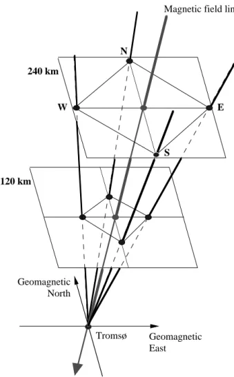
Fig. 1. An illustration of the idealized EISCAT radar mode. The
transmitting antenna is sequentially pointed to four positions. Ide-ally, two pairs of the four directions would form the two orthogonal diagonals of a square. In each of the four positions, the electric field in the F-region (240 km) is measured with three antennas, and the Pedersen and Hall conductivities are determined along the Tromsø beam.
distribution of FACs on a summer day, which was in gen-eral agreement with that derived statistically by Iijima and Potemra (1976). Sorting by the geomagnetic activity index
Kp, Fontaine and Parmirat (1996) showed statistical distri-butions of the horizontal currents and FACs that were based on models of the large-scale convection (Senior et al., 1990) and conductance (Senior, 1991) derived statistically from ob-servations with the EISCAT radar.
These studies based on IS radar measurements are mainly concerned with the large-scale global distribution of FACs. However, they employed meridian scanning modes, and the Earth’s rotation was utilized for obtaining longitudinal dis-tributions. Thus, the global distribution obtained can be jus-tified only when it has negligibly small temporal variations. In order to understand more accurately how the FAC is con-nected to its closure current and the relative contribution of ionospheric parameters to the FAC, a two-dimensional
mea-surement within the time scale of the variations is essential. Also, differences in the Pedersen and Hall current contribu-tions to FACs are of great interest.
Based on an algorithm by Amm (1998), Kosch et al. (2000, 2001) showed the FAC distribution of a plasma flow vortex associated with the brightening of an auroral arc. They il-lustrated that the downward current region resulted mostly from diverging horizontal Pedersen currents. Assuming a Hall-to-Pedersen conductance ratio, they estimated conduc-tances from the Scandinavian Magnetometer Array (SMA) (K¨uppers et al., 1979) and Scandinavian Twin Auroral Radar Experiment (STARE) (Greenwald et al., 1978) data. Al-though STARE is a powerful tool to obtain two-dimensional maps of the electric field, it can provide reliable ionospheric electric fields only when they exceed 15 mV/m (Cahill et al., 1978). As shown by several studies, the conductance and the electric field closely interact with each other (e.g. de la Beau-jardi`ere et al., 1981; Baumjohann, 1983; Marklund, 1984). Hence, it is indispensable to measure these parameters si-multaneously and precisely for a better understanding of the three-dimensional current systems.
A merit of using the EISCAT radar is that we can accu-rately measure temporal and spatial variations of both the conductance and the electric field. In order to determine how the ionospheric current is connected to the FAC quan-titatively, we made a special experiment with the EISCAT radar on 9 October 1999. Since the proposed method to de-termine the FAC must be validated as to whether it provides a meaningful current density or direction, a comparison study based on simultaneous observations with other instruments is important. We present a comparative study using simulta-neous observations, such as auroral images and satellite data. An enhancement of the ionospheric electron density or the Pedersen conductivity is generally seen in an upward FAC re-gion due to auroral precipitation. The paired downward FAC is expected to require a larger ionospheric electric field than the upward FAC, to close the ionospheric current connect-ing different Pedersen conductivity regions. Low-altitude satellite observations show that some kind of upward FACs with intense precipitation are associated with smaller elec-tric fields; sometimes the elecelec-tric field appears to be even short-circuited (e.g. Hoffman, 1989). This relatively small electric field is usually considered to be the combination of the magnetospheric electric field and the polarization electric field produced by the charge accumulation due to the inho-mogeneity of the ionospheric conductivity (e.g. Baumjohann et al., 1983). It should be emphasized that the polarization electric field, arising from the density inhomogeneity in the polar ionosphere, can drive FACs of ionospheric origin. The polarization electric field can play a role in the re-distribution of the electric field and hence, the modification of the current systems (e.g. Lysak, 1990). Although the development of the polarization electric field is discussed theoretically, it has not been well understood observationally. Thus, the investi-gation of the electric fields associated with auroral arcs also enables us to understand how ionospheric closure currents and FACs are distributed around auroral arcs.
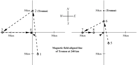
1 3 2(Tromsø) Magnetic field-aligned line of Tromsø at 240 km 5 7 6 8 50km 50km 50km 50km 50km 50km 50km 50km (Tromsø) 4 N S E W
Fig. 2. Beam positions at 240 km height in the mode employed, taking into account the Earth’s rotational effect. The spatial scale for electric
field measurements at 240 km height is 100 km in the first set of beams (1–2–3–4), and 50 km in the second set (5–6–7–8). The spatial scale for the conductance measurement becomes 50 (25) km in the first (second) set.
Kosch et al. (2000) showed the region of diverging iono-spheric electric fields associated with a sudden brightening of the arc. They suggested that the region corresponded to a downward FAC and black auroras; however, no black au-roras could be identified in their all-sky TV data, owing to its limited resolution. Using an all-sky camera and the EIS-CAT radar, Lewis et al. (1994) revealed the presence of a band of enhanced electric field on only one side of a drifting auroral arc, but its development was not detected by all-sky camera images. Although several studies have reported the characteristics of a region with an enhanced electric field, its temporal development is still not clear. Based on both EIS-CAT radar measurements and auroral images, we also focus on the temporal or spatial variation of the region with high electric fields associated with auroral arcs.
2 EISCAT radar mode employed
In this study we have used the tristatic European Incoher-ent Scatter (EISCAT) radar, the so-called Kiruna-Sodankyl¨a-Tromsø (KST) UHF radar system (Folkestad et al., 1983; Rishbeth and Williams, 1985). Scattered signals from the radar beam transmitted at Tromsø (69.6◦N, 19.2◦E, 66.2◦ invariant latitude) are received at three stations; Tromsø it-self, Kiruna, and Sodankyl¨a, and thus, the three-dimensional ion velocity can be calculated. The electric field (E) can be determined from the three-dimensional ion velocity at an altitude (240 km in our mode) in the F-region, where ions move by E × B drift, since the ion gyrofrequency is much greater than the ion-neutral collision frequency here. The magnetic field (B) is derived from the International Geomag-netic Reference Field (IGRF) model (Barton, 1997). Along the Tromsø beams, EISCAT radar measurements also pro-vide the electron density and ion/electron temperatures with a height resolution of about 3 km in the E-region, and of about 20 km in the F-region. Thus, the Pedersen and Hall
conductivities (σP and σH) can be calculated using formulas by Brekke and Hall (1988) and the MSISE-90 neutral atmo-spheric model (Hedin, 1991). The Pedersen and Hall con-ductances (6P and 6H) are calculated by integrating them over the height range from 90 to 300 km. The adoption of the lower height limit of 90 km may be justified, except under extremely energetic precipitation, which could pro-duce as much as 15% of the Hall conductance below 90 km (Schlegel, 1988). From these ionospheric parameters we can derive the ionospheric current (J ) as,
J = JP +JH =6PE + 6H(b × E) , (1)
where JP and JH are the height-integrated Pedersen and Hall currents, respectively, and b is the unit vector in the di-rection of the Earth’s magnetic field. The experiment also enables us to determine the relative contribution of the gradi-ent of the ionospheric conductance and the divergence of the electric field to the FAC density jk(positive away from the ionosphere) in the following way,
−jk=div J = 6Pdiv E + E · grad 6P
+(b × E) · grad 6H+6Hdiv (b × E) . (2)
Each of these terms depends on both the electric field and the conductance. The first term depends on the divergence of the electric field, and is called the term of “magnetospheric origin FAC” (e.g. Sofko et al., 1995). The second and third terms, called the terms of “ionospheric origin FAC”, depend on the gradient of Pedersen and Hall conductances, respec-tively. Since our method assumes that the ionospheric elec-tric field is a curl-free potential elecelec-tric field (rot E = 0), the last term should be zero.
In order to derive the gradient of the ionospheric conduc-tance and divergence of the electric field, we conducted a special experiment using the EISCAT radar. Figure 1 is an il-lustration of the idealized EISCAT radar mode. The transmit-ting antenna is sequentially pointed to four positions, similar
50 0 nT 20 21 22 23 00 01 02 03 -1000-800 -600 -400 -2000 200 400 Y X Z 20 21 22 23 00 01 02 03 UT (hour) (a) (b)(c) (d)(e) AU AL [nT]
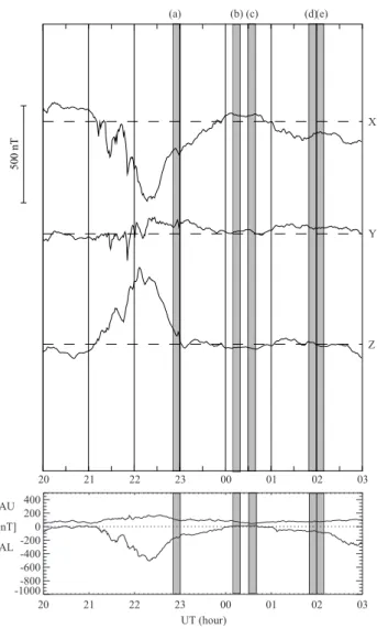
Fig. 3. Ground-based magnetometer data at Tromsø (upper) and the
AU − ALindex (lower) during our experiment.
to CP-2 mode (see e.g. Collis, 1995). Ideally, two pairs of the four directions would form the two orthogonal diagonals of a square, as illustrated in Fig. 1. In each of the four positions, the electric field in the F-region (240 km) is measured with the three antennas, and the Pedersen and Hall conductivities are determined along the Tromsø beam.
The Earth rotates once a day under the ionosphere with the rotation speed of about 10 km/min at Tromsø (69.6◦N). Tak-ing into account this rotational effect, we designed our radar mode to make the four beam positions form a square in the ionosphere, where the patterns of the electric field (equiva-lently the plasma convection) and precipitation (the auroral oval) do not move with the Earth’s rotation, but rather are fixed in the Sun-Earth coordinates. Figure 2 illustrates the beam positions at 240 km height in our special radar mode employed. It is noted that the transmitting antenna is di-rected nearly along the geomagnetic field in the beam po-sition 4. Also, beam 2 points vertically upward. When the transmitting antenna is not directed along the magnetic field line at Tromsø , the measurements in the E- (conductances)
and F- (electric fields) regions are not on the same magnetic field line. However, this may not be a serious problem if the electric field and the ionospheric conductances are linearly varying in the square region concerned, which is implicitly assumed in this method.
What we are able to derive is, for example, the divergence of the electric field with the spatial scale approximately the same as, or larger than, the spatial size of the square ob-serving region. Contributions from smaller scale variations cannot be taken into account. In our radar mode we alter-nately measured two sets of the four beam directions, in or-der to investigate the distributions of the parameters in dif-ferent spatial scales. As shown in Fig. 2, the spatial scale for electric field measurements at 240 km height is 100 km in the first set of beam positions (1–2–3–4), and 50 km in the second set (5–6–7–8). The height-dependent Pedersen con-ductivity is typically largest around 120 km in height. Hence, the adopted spatial scale for the conductance measurement becomes 50 km in the first set and 25 km in the second set. The time resolution of the post-integrated parameters is about 2 min. To complete one antenna cycle consisting of four posi-tions requires 10 min, which may allow us, under some con-ditions, to assume that the measured distribution is a spatial distribution without temporal variations.
3 Observations
We conducted our experiment with the EISCAT radar from 20:30 UT on 9 October to 02:30 UT on 10 October 1999. Figure 3 shows the ground-based magnetometer data at Tromsø (upper panel) and AU −AL index (lower panel) dur-ing this experiment. A relatively quiet period can be seen, except from 21:00–24:00 UT, when disturbances due to sub-storms are identified. The geomagnetic disturbance level is
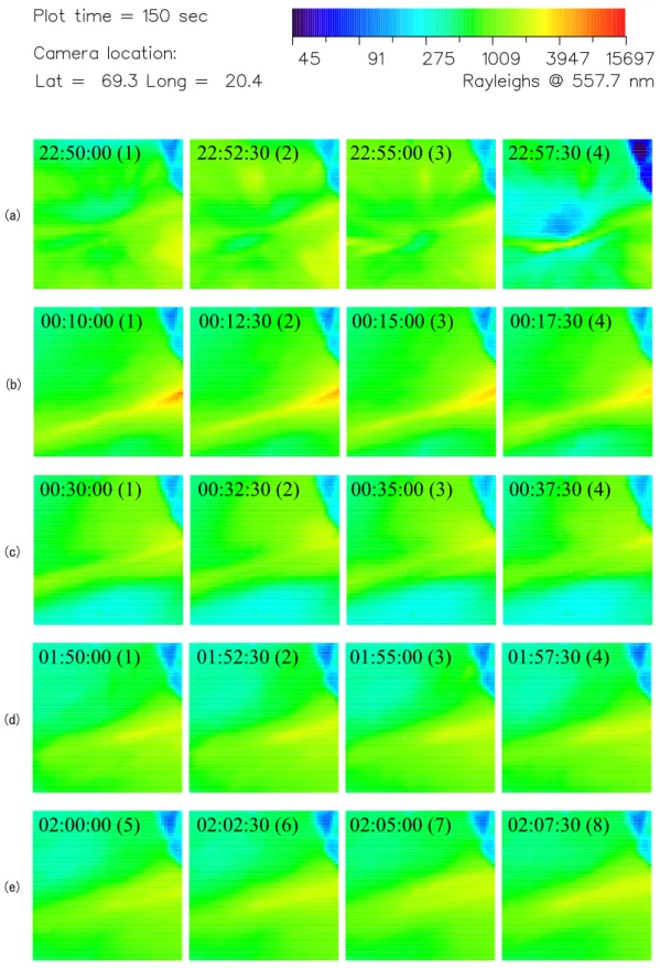
Kp = 3− (18:00–21:00 UT on 9 October, 00:00-03:00 UT on 10 October) and Kp=3 (21:00–24:00 UT on 9 October). Since our method to calculate a FAC density assumes lit-tle temporal variations within 10 min, we selected suitable time periods from the whole experiment interval by checking the digital all-sky imager (DASI) data (Kosch et al., 1998a). Figure 4 shows all-sky images of the selected events we will present later. Little temporal variations are seen, ex-cept in case (a). The all-sky camera is located at 69.3◦N, 20.4◦E, about 50 km from the EISCAT transmitter. The spatial coverage is 67.6–72.6◦N, 13.5–26.0◦E geographic (about 520 × 520 km) with 10 × 10 km resolution. The co-ordinates used here are positions mapped to a 100 km alti-tude. The intensity is calibrated in Rayleighs for 557.7 nm. The observation starting time (UT) and beam position cor-responding to numbers (1–8) in Fig. 2 are noted in the top of each image of Fig. 4. The white dot near the center of each image is the position of the EISCAT radar beam (not radar site) at 100 km altitude. Thus, the white dot shows the point where the ionospheric conductance is precisely ob-served, and it shifts sequentially along with the beam
scan-22:50:00 (1)
22:52:30 (2)
22:55:00 (3)
22:57:30 (4)
C00:10:00 (1)
00:12:30 (2)
00:15:00 (3)
00:17:30 (4)
00:30:00 (1)
00:32:30 (2)
00:35:00 (3)
00:37:30 (4)
D E01:50:00 (1)
01:52:30 (2)
01:55:00 (3)
01:57:30 (4)
02:00:00 (5)
02:02:30 (6)
02:05:00 (7)
02:07:30 (8)
F GFig. 4. All-sky images of the selected events. The spatial coverage is 67.6–72.6◦N, 13.5–26.0◦E geographic (about 520 × 520 km) at 10 × 10 km resolution. Mapping is for 100 km altitude. The intensity is calibrated in Rayleighs for 557.7 nm. The white dot near the center of each image is the position of the EISCAT radar beam at 100 km altitude. The observation starting time (UT) and beam position corresponding to numbers (1–8) are noted in the top of each image. The dark triangle in the top right corner of every image is the mountain near Skibotn, Norway.
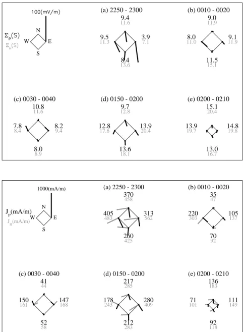
S N W E (a) 2250 - 2300 8.4 13.6 9.4 11.6 9.5 11.3 3.97.1 (b) 0010 - 0020 11.5 15.1 9.0 11.9 8.0 11.0 11.99.1 (c) 0030 - 0040 8.0 8.9 10.8 11.6 7.8 8.4 8.29.4 (d) 0150 - 0200 13.6 18.1 9.7 12.8 12.8 17.6 13.920.4 (e) 0200 - 0210 13.0 16.7 15.1 20.4 13.9 19.7 14.819.8
Fig. 5. Spatial variations of the
con-ductance and the electric field observed with the EISCAT radar. Each position of the quadrilateral corresponds to the four beam positions, respectively; bot-tom (south, beam 1 or 5), top (north, beam 2 or 6), left (west, beam 3 or 7), and right (east, beam 4 or 8). Each thick line indicates the strength and direction of the electric field. The Pedersen (up-per) and Hall (lower) conductances are denoted in the unit of S.
S N W E 1000(mA/m) J P(mA/m) J H(mA/m) (a) 2250 - 2300 260 425 370 458 405 483 313562 (b) 0010 - 0020 70 92 35 47 220 303 105137 (c) 0030 - 0040 52 58 41 44 150 161 147168 (d) 0150 - 0200 212 283 217 285 178 243 280409 (e) 0200 - 0210 92 118 136 183 71 101 111149
Fig. 6. Spatial variations of the cal-culated height-integrated Pedersen and Hall currents, assuming that both of the conductance and the electric field are measured on the same magnetic field line. Each thick (thin) line indicates the strength and direction of the Pedersen (Hall) current.
ning. The dark triangle in the top right corner on each image is a mountain near Skibotn, Norway.
Figure 5 shows spatial variations of the conductance and the electric field observed with the EISCAT radar in the se-lected cases corresponding to Fig. 4. Each position of a quadrilateral corresponds to the four beam positions, respec-tively; bottom (south, beam 1 or 5), top (north, beam 2 or 6), left (west, beam 3 or 7), and right (east, beam 4 or 8). Each thick line denotes the strength and direction of the electric field. The Pedersen (upper) and Hall (lower) conductances are also denoted in the unit of S. Note that, except for the beam 4, the measurements of conductances and electric fields are not on the same magnetic field line. Using an approxima-tion that both the conductance and electric field are measured on the same magnetic field line, we present spatial variations of the calculated height-integrated Pedersen (JP) and Hall (JH) currents in Fig. 6. Each thick (thin) line indicates the
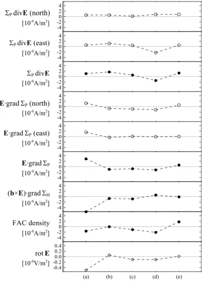
strength and direction of the Pedersen (Hall) current. Figure 7 presents the calculated FAC density using the for-mula (2). Each term (except the last term) of the forfor-mula (2) and the total FAC density are plotted. Also, northward and eastward components of 6P div E and E · grad 6P are shown. A positive value means an upward current density. In order to examine how temporally stable the ionospheric parameters are, rot E is also plotted. Ideally, rot E becomes zero. The greater the amplitude of rot E is, the less valid our assumption becomes.
4 Results
In case (a), during 22:50–23:00 UT, a lot of temporal varia-tions are seen in the aurora camera, as depicted in the top four panels of Fig. 4. At first, we will present the cases in which
( a) (b) ( c) ( d) (e) -4 -20 2 4 [10-6A/m2] ( a) (b) ( c) ( d) (e) -4 -20 2 4 [10-6A/m2] ( a) (b) ( c) ( d) (e) -4 -20 2 4 [10-6A/m2] ( a) (b) ( c) ( d) (e) -4 -20 2 4 [10-6A/m2] ( a) (b) ( c) ( d) (e) -4 -20 2 4 [10-6A/m2] ( a) (b) ( c) ( d) (e) -4 -20 2 4 [10-6A/m2] ( a) (b) ( c) ( d) (e) -4 -20 2 4 [10-6A/m2] ( a) (b) ( c) ( d) (e) -4 -20 2 4 [10-6A/m2] (a) (b) (c) (d) (e) -0.4 -0.20.0 0.2 0.4 [10-6V/m2]
Fig. 7. Calculated FAC densities
de-duced from EISCAT radar measure-ments. Each term (except the last term) of the formula (2), the total FAC den-sity, and rot E are plotted. Also, north-ward and eastnorth-ward components of 6P div E and E · grad 6P are plotted. A positive value means an upward current density.
the ionosphere is relatively stable, and then discuss the case (a).
4.1 Cases (b) 00:10-00:20 UT and (c) 00:30-00:40 UT on 10 October 1999
The EISCAT radar observed a region around a relatively small-scale auroral arc. Both the ground-based magnetome-ter data in Fig. 3 and auroral images in Figs. 4b and c indicate that temporal variations are small during these time periods. During 00:10–00:20 UT in Fig. 5b, the conductance in the south position is larger than that in the other three positions, with a small electric field. An anti-correlation between the conductance and the electric field strength is seen. This has been reported as one of the common features of auroral arcs (e.g. Baumjohann, 1983; Marklund, 1984). Figure 4b con-firms that the arc is located at the southward position of the larger square formed by the four beam directions. While the electric field in the north position is also small, with a low conductance, however, this seems due to the large distance between the north position and the arc (100 km at 240 km al-titude). This small electric field in the north position implies that the background convection electric field is also small.
On the other hand, in the vicinity neighboring the arc, the electric field is enhanced with a low conductance in the east and west positions.
During 00:30–00:40 UT in Fig. 5c, a conductance en-hancement can be seen in the north position with a small electric field. Figure 4c depicts a narrow arc similar to that shown in Fig. 4b, however, the arc is located in the north of the region measured with the EISCAT radar. Also, in the vicinity of the arc, enhancements of the electric field can be seen.
In summary, during these periods, the relatively high elec-tric field associated with the narrow arc is confined to a spa-tially restricted region, within 100 km from the arc. This arc-associated electric field is rather stable. In Fig. 7 for cases (b) and (c), 6P div E produces an upward FAC, while
E · grad 6P produces the opposite direction of the FAC.
4.2 Cases (d) 01:50-02:00 UT and (e) 02:00-02:10 UT on 10 October 1999
The EISCAT radar surveyed a region around a broad auroral band. Both ground-based magnetometer data at Tromsø in Fig. 3 and auroral images in Figs. 4d and e suggest that the
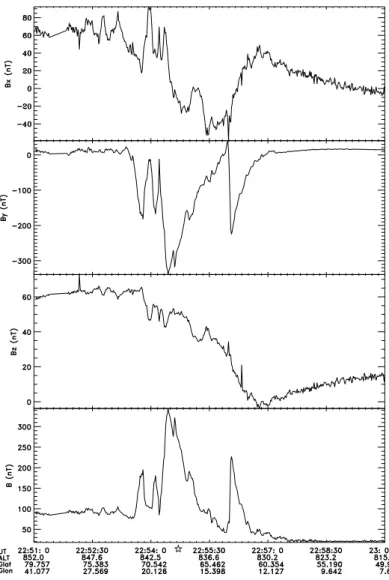
Fig. 8. Magnetic field measurements
obtained by the flux-gate magnetome-ter carried on the Ørsted satellite. Bx, By, Bz and B are shown after sub-traction of the preliminary Ørsted main field model, where X is positive geo-graphic north, Y is positive east, Z is positive down, and B is the total mag-netic field strength. The closest position of the EISCAT radar is indicated by the star.
temporal variation is also small during these periods. The thickness of the auroral arc is larger compared with the arc seen in the previous cases (b) and (c), and its border is not so well defined. The AU − AL index in Fig. 3 suggests that these cases are during what appears to be a prolonged growth phase of a minor substorm.
During 01:50–02:00 UT, the conductances in the south and east positions are larger than those in the other two positions in Fig. 5d. The electric field is also not small with high con-ductances. This feature is different from that in the previous cases, which showed an anti-correlation between the conduc-tance and the electric field. Figure 4d suggests that the EIS-CAT radar sounded a region northwestward of the broad arc. On the other hand, during 02:00–02:10 UT, the conduc-tivity is high and has the maximum in the north position in Fig. 5e. The electric field is small on each of the four po-sitions, suggesting that the EISCAT radar sounded a region inside of the broad arc. This is confirmed by the auroral im-ages in Fig. 4e. It is noted that, in case (e), the EISCAT radar measured a smaller square region formed by the beam posi-tions 5–8.
As shown in Fig. 7, for cases (d) and (e), a downward FAC
appears in the north of the arc during 01:50–02:00 UT, and an upward FAC inside the arc during 02:00–02:10 UT. In cases (d) and (e), both 6P div E and E · grad 6P produce the same direction FAC. On the other hand, (b × E) · grad 6H is small and not effective in closing the FAC. Hence, the divergence of the electric field and the gradient of the Pedersen conduc-tance play a significant role in closing the FAC through the ionosphere.
In Fig. 5, except in case (a), one notices that all of the stable arcs have a conductivity gradient in the east-west di-rection and that the conductivity in the east position is higher than that in the west position in each case. Also in Fig. 4, the stable arcs are brighter toward the east. From the viewpoint of the current closure in the ionosphere, however, the conduc-tivity gradient in the north-south direction plays a more cru-cial role than that in the east-west direction, since the north-south component of the electric field is generally larger than the east-west component, as seen in Fig. 5. Hence, the term
E · grad 6P is highly dependent on the north-south
gradi-ent of the ionospheric Pedersen conductivity. While the term (b×E)·grad 6Hdepends mainly on the east-west gradient of the ionospheric Hall conductivity, this gradient is not so large
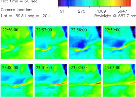
22:56:00 22:57:00 22:58:00 22:59:00
23:00:00 23:01:00 23:02:00 23:03:00
Fig. 9. All-sky images with a time resolution of 1 min, around the time when a dark spot was observed.
compared with the north-south gradient of the Pedersen con-ductivity, as shown in Fig. 5e. Thus, the FACs close through the Pedersen current rather than through the Hall current in the ionosphere in this specific case.
4.3 Case (a) 22:50-23:00 UT on 9 October 1999
During this time period, the Ørsted satellite passed over the EISCAT radar at 22:54 UT. The magnetic field measurements obtained from the fluxgate magnetometer carried on board the Ørsted satellite are shown in Fig. 8. Bx, By, Bz and
B are magnetic fields after subtraction of the Earth’s main fields from the observed magnetic fields, where X is geo-graphic north, Y is east, Z is down, and B is the total mag-netic field strength, B = (Bx2+By2+Bz2)1/2. Notice that the largest perturbations are seen in the Y -direction, indicating that the Ørsted trajectory is nearly perpendicular to the FAC sheets. The Ørsted observation indicates that a large-scale downward FAC region is located between about 72.6◦N and 69.0◦N, while an upward FAC region is located between about 69.0◦N and 63.5◦N. The nearest position to the EIS-CAT radar (indicated by the star in Fig. 8) is located at the separation between the two large-scale current sheets. When the Earth rotates and a substorm evolves, the EISCAT radar appears to be shifted back and forth between the two FAC re-gions. In the vicinity of the EISCAT radar, the Ørsted satel-lite observes many small-scale FACs within the large-scale FACs. This is a common feature of an auroral substorm dur-ing this MLT (e.g. Fujii et al., 1994). The AU − AL index in Fig. 3 also suggests that this case (a) is during the late recovery phase of a substorm.
Several temporal variations are seen in the auroral images, as depicted in Fig. 4a. Especially in the east position (22:58– 23:00 UT), the auroral image shows a dark spot adjacent to
a narrow bright arc. Correspondingly, the EISCAT radar de-tects a very high electric field (∼ 80 mV/m) and low conduc-tances in this position, as exhibited in Fig. 5a. This elec-tric field seems unstable and different from the arc-associated electric fields, as shown in cases (b) and (c), which are rather stable. We have selected this case (a) because a noteworthy dark spot was detected. It should be noted that the FAC cal-culated from the four position measurements with the EIS-CAT radar is probably not accurate because this case vio-lates the necessary assumption of no temporal variation over 10 min. This is confirmed by the calculation of rot E, which is much larger than in the other cases shown in Fig. 7.
With a time resolution of 1 min, Fig. 9 depicts the de-tailed temporal variation of the dark spot around the observed time. The dark spot is clearly identified only during 22:58– 2:300 UT, drifting eastward slowly. Simultaneously, a nar-row bright arc appears southward of the dark spot. Also south of the arc, a narrow dark region can be seen during 22:58– 22:59 UT. We observed another dark spot around 21:46 UT (not shown here) also lasting for a limited time of a few min-utes.
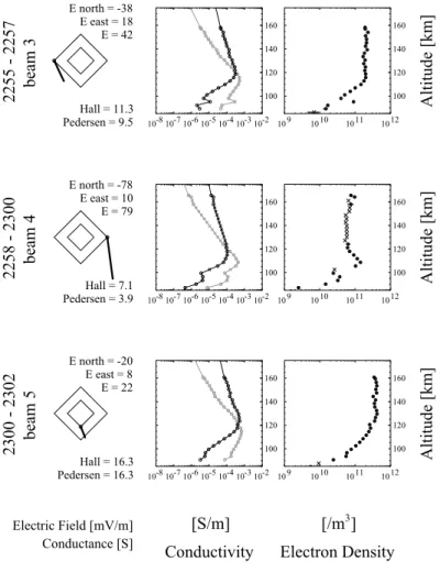
Figure 10 shows EISCAT radar measurements of the height distribution of the Pedersen (thick line) or Hall (thin line) conductivity and the electron density. During 22:58– 23:00 UT, the EISCAT radar sounded inside of the dark spot, as shown in Fig. 4a, with the field-aligned beam position 4. The low conductances and the enhanced electric field can be seen. The electric field is directed to the narrow arc, and thus, the Pedersen current also flows from the dark spot to-ward the arc. Above 110 km altitude, the electron density is depleted. The measurements at several altitudes are missing due to weak backscatters from low electron densities with relatively large errors (as denoted by the crosses in Fig. 10). Such a depletion especially leads to a reduction of the
Ped-ersen conductivity, since it has a maximum around 120 km altitude. As seen in Fig. 4a, the beam position 4 is south of the darkest area in the dark spot, where the maximum de-pletion of electron density occurs and thus, the more intense downward FAC are expected.
5 Discussion
5.1 Stable narrow arc
In cases (b) and (c), the stable electric field associated with the narrow arc is confined to a spatially restricted region, within ∼ 100 km from the arc. Based on radar measurements, a number of studies have reported features of arc-associated electric fields. Aikio et al. (1993) showed that the width of an arc-associated electric field was estimated to be less than, or equal to, 45 km. Opgenoorth et al. (1990) suggested that the width of very high perpendicular electric fields, as-sociated with a reduced electron density, was estimated to be of the order of the arc width (about 20 km). Lewis et al. (1994) estimated the horizontal extent of the electric field to be about 40 km. It is also noted that the arc-associated electric field shown by Opgenoorth et al. (1990) or Lewis et al. (1994) accompanies a reduction of the electron den-sity, while our observed arc-associated electric field in cases (b) and (c) is not accompanied with such a strong reduction. Past studies showed that the arc-associated electric field was observed only on one side of the narrow arc. Baumjohann (1983) has explained that the ambient electric field is north-ward (southnorth-ward) directed in the evening (morning) sector and thus, the arc-associated meridional electric field must be anti-symmetric with respect to the southern (northern) bor-der of the arc, being northward (southward) directed in a region a few kilometers south (north) of the arc and south-ward (northsouth-ward) inside the arc. However, our observation in cases (b) and (c) exhibits the arc-associated electric field on both the northward and southward sides outside the narrow arc. On both sides, the arc-associated electric field directs towards the narrow arc in a spatially restricted region. This feature is rather similar to that of the event shown by Burch et al. (1976), who determined the characteristics of pairs of op-positely directed spikes in ionospheric convection velocities using data from AE-C spacecraft. Their convection velocities are associated with the inverted-V type auroral electron pre-cipitation. They suggested that the relationship between the electron precipitation and the electric field spikes was consis-tent with an upward-flowing FAC that was fed by Pedersen currents from the adjacent regions of strong convection.
In Fig. 7, for cases (b) and (c), 6P div E produces an upward FAC, while E · grad 6P produces an opposed down-ward FAC. Sato et al. (1995) have reported a similar situ-ation at the equatorward edge of the large-scale downward region 1 current. A small rot E in Fig. 7 for cases (b) and (c) shows that the temporal variation is small. However, it is suspected that the region observed with the EISCAT radar includes both upward and downward FAC regions in these
cases. As described by Marklund (1984), if a transverse height-integrated current has a difference between two ob-served positions, there is a FAC between the two. For ex-ample, in Fig. 6c, the Pedersen current in the west or east position is larger (∼ 150 mA/m) than that in the south or north position (∼ 50 mA/m). This implies that a northwest-ward Pedersen current (∼ 150 mA/m) flows in the center of the four observed positions. Thus, it is expected that FACs flow upward in the northern half of the four positions, and downward in the southern half. Similarly in Fig. 6b, a south-eastward Pedersen current is expected to flow in the center of the four positions, with an upward FAC in the northern half and a downward FAC in the southern half. Thus, we con-clude that the spatial scale of the region observed with the EISCAT radar was too large in comparison to the spatial cur-rent structure, in order to apply formula (2) reliably for cases (b) and (c). In these cases, we cannot confirm whether 6P div E and E · grad 6P really produce FACs with opposing directions, as reported by Sato et al. (1995).
5.2 Stable broad arc
As shown in Fig. 7, for cases (d) and (e), a downward FAC is inferred to exist north of the arc, and an upward FAC inside the broad arc. In cases (d) and (e), both 6P div E and E · grad 6P produce the same direction FAC. Only in the north-south direction, in case (e), 6P div E and
E·grad 6P produce FACs with opposing directions, in
agree-ment with the result by Sato et al. (1995). On the other hand, (b × E) · grad 6H is small and not effective in closing the FAC.
In Fig. 4e, the aurora moves slightly westward with the passage of time, keeping its form, and is favorable for our radar mode, taking into account the Earth’s rotational effect. Also in case (e), the area scanned by the beam positions 5– 8 is small (see Fig. 2) and the calculated rot E is extremely small (see Fig. 7). Therefore, the situation in case (e) is the most appropriate one out of all our cases, in order to calculate a FAC using formula (2). The calculated FAC is also the most reliable in case (e) rather than that in any of the other cases. The upward FAC density by 6P div E and E · grad 6P are
∼1.3 and ∼ 0.7 µA/m2, respectively, and thus the contribu-tion of 6Pdiv E is nearly twice as large as that of E·grad 6P in case (e).
These results are consistent with the results by Kosch et al. (2000) and Kosch and Nielsen (2001). However, they dis-cussed a plasma vortex associated with a black aurora, which seems similar to the dark spot shown in case (a). Our results are based on observations of the stable arc around 02:00 UT (∼ 05:00 MLT) in cases (d) and (e). We have also checked several auroral images and could find auroral forms with the same features in the early morning on other days (not shown here). Thus, the arc in cases (d) and (e) is considered to be a common feature seen in the early morning. Unfortunately, the electric fields in these cases are not very large, and thus, it is difficult for STARE to measure reliable electric fields
Electric Field [mV/m] Conductance [S] [S/m] Conductivity [/m3] Electron Density 22 55 - 22 57 be am 3 E north = -38 E east = 18 E = 42 Hall = 11.3 Pedersen = 9.5 10-8 10-7 10-6 10-5 10-4 10-3 10-2 100 120 140 160 100 120 140 160 109 1010 1011 1012 100 120 140 160 100 120 140 160 A lti tu de [k m ] 22 58 - 23 00 be am 4 E north = -78 E east = 10 E = 79 Hall = 7.1 Pedersen = 3.9 10-8 10-7 10-6 10-5 10-4 10-3 10-2 100 120 140 160 100 120 140 160 109 1010 1011 1012 100 120 140 160 100 120 140 160 A lti tu de [k m ] 23 00 - 23 02 be am 5 E north = -20 E east = 8 E = 22 Hall = 16.3 Pedersen = 16.3 10-8 10-7 10-6 10-5 10-4 10-3 10-2 100 120 140 160 100 120 140 160 109 1010 1011 1012 100 120 140 160 100 120 140 160 A lti tu de [k m ]
Fig. 10. EISCAT radar measurements
of the altitude profile of the Pedersen (thick line) and Hall (thin line) conduc-tivities and the electron density, around the time when a dark spot was observed.
and to deduce the FAC density, as demonstrated by Kosch et al. (2000).
Two major high-latitude FAC systems have been statisti-cally shown to exist (Iijima and Potemra, 1976). In the dawn sector, the poleward currents, denoted as region 1 currents, flow into the ionosphere, and the equatorward currents, de-noted as region 2 currents, flow away from the ionosphere. This distribution is consistent with our calculated FAC in cases (d) and (e), which is downward north of the stable arc, and upward to the south. In Fig. 3, the ground mag-netometer observation around 02:00 UT indicates 1Z ∼ 0, meaning that the electrojet current center may be located near Tromsø. In the morning sector, Senior et al. (1982) and Sato et al. (1995) have inferred that the center of the west-ward electrojet current is located near the region 1/region 2 FAC reversal. Thus, the ground magnetometer data showing
1Z ∼0 are consistent with our calculated FAC distribution. The estimated FAC densities (∼ 2 µA/m2) have the same or-der as the reported FAC densities by satellite observations (e.g. Iijima and Potemra, 1978; Fukunishi et al., 1993).
In Fig. 5, except in case (a), all of the stable arcs have a conductivity gradient in the east-west direction, and the con-ductivity in the east position is higher than that in the west position in each case. Also in Fig. 4, the stable arcs are brighter towards the east. This indicates that particle
precip-itation, which is effective in enhancing ionospheric conduc-tivities, should be greater going from midnight to the dawn side. As mentioned before, we see similar stable arcs in au-rora images on other days, and the stable arcs in Fig. 4 are thus considered to be a common feature around these MLTs. In the ionosphere, the conductivity is well determined by the precipitating electron energy and electron energy flux (e.g. Spiro et al., 1982; Robinson et al., 1987; Hardy et al., 1987). The conductivity gradient in the north-south direc-tion plays a crucial role in producing the FAC rather than that in east-west direction, as mentioned before. On the other hand, in the magnetosphere, the plasma pressure is con-tributed mainly by hot ions (e.g. Spence et al., 1989). In the magnetosphere, a pressure-gradient force on the plasma in the equatorial plane plays a crucial role on FAC generation (e.g. Iijima, 2000).
5.3 Narrow bright arc and dark spot
In case (a), we see a region with a very high electric field adjacent to a narrow bright arc. In the auroral images, this region is identified as a dark spot. The region is estimated to have a spatial dimension, over 150 × 150 km, that is much larger than that reported for “black auroras” (see a brief re-view by Kosch et al., 1998b). This implies that our observed
dark spot may be different from phenomena of black auro-ras. According to the definition, the black aurora is a lack of emission in a small, well-defined region within an otherwise uniform, diffuse background or within auroras exhibiting a degree of shear behavior intermediate between that of dif-fuse and discrete aurora (see Trondsen and Cogger, 1997). Black auroras appear to be a common feature of the late re-covery phase of an auroral substorm. Several high spatial and temporal resolution optical observations have identified black auroras. Schoute-Vanneck et al. (1990) measured 40 black filaments to find a typical width of 1 km, and length of 5–20 km. Trondsen and Cogger (1997) measured 31 black auroral patches and arc segments and found a typical width of 0.5–1.5 km.
On the other hand, the plasma vortex analyzed by Kosch et al. (2000) has a spatial dimension, 200 × 200 km, which is of the same order as our observed dark spot. If the dark spot is a similar feature of the plasma vortex shown by Kosch et al. (2000), a downward FAC is expected in the dark spot. In-deed, our observed depletion of electron density over 110 km altitude implies that the dark spot occurs in the downward FAC, which carries ionospheric electrons into the magneto-sphere as a current carrier. As mentioned before, the po-sition observed by the beam 4 is on the south side of the darkest point in the dark spot, where the greatest depletion of electron density occurs and thus, the more intense downward FAC is expected. In the case analyzed by Kosch et al. (2000), the strongest downward FAC in the center of the plasma vor-tex is also far from the bright arc (∼ 100 km).
There may be an alternative explanation for the electron density depletion within the dark spot. High electric fields can alter the ion composition and also lead to an electron density decrease due to enhanced recombination. According to the result by Schunk et al. (1975), this decrease is seen mainly in the F-region, however, it is noted that the density depletion we detected within the dark spot is seen also in the E-region (above 110 km).
When the dark spot is identified, a narrow bright arc appears simultaneously south of the dark spot. Aikio et al. (1993) have reported the simultaneous intensification of the arc-associated electric field and the optical brightening of the auroral arc. Due to the beam swing, the EISCAT radar could observe both inside the dark spot and the narrow arc. During 23:00–23:02 UT, the EISCAT radar sounded inside the narrow arc with the beam position 5. Both the Peder-sen and Hall conductances increase with a smaller electric field. Moving from inside the dark spot to inside the narrow arc, the height-integrated Pedersen current does not change much. In our case (a), the electric field points from the dark spot into the narrow arc; thus, one can conclude that the Ped-ersen current is the closure current between the dark spot and the narrow arc. Using the observed conductance and the elec-tric field, we can quantitatively estimate the height-integrated Pedersen and Hall currents; 310 and 560 mA/m inside the dark spot during 22:58–23:00 UT, and 360 and 360 mA/m inside the narrow arc during 23:00–23:02 UT, respectively. The difference in the Pedersen and Hall currents between the
two regions is 50 and 200 mA/m, respectively. It should be noted, however, that these values have some ambiguity, be-cause there is a time lag between observations of the two re-gions. The dark spot became fainter when the EISCAT radar measured inside the narrow arc during 23:00–23:02 UT. This may imply that the current morphology changes. Also, in-side the narrow arc, the conductivities and the electric field are not measured on the same magnetic field line by the beam position 5. This may add an error to the calculated current in-side the arc. However, this difference in the Pedersen current is smaller than that of about 100 mA/m in case (b).
5.4 EISCAT radar mode employed and future
The neutral wind cannot be measured in our observations, and is neglected in the present analysis. In the ionosphere, the electric field is the sum of the potential electric field (de-rived from the plasma motion in the F-region) and the neutral dynamo electric field U × B, where U is the neutral wind ve-locity. The neutral wind velocity varies greatly with altitudes in the E-region (e.g. Nozawa and Brekke, 1995); thus, the dynamo electric field U ×B is also highly altitude dependent. The amplitude of the dynamo electric field occasionally be-comes comparable to that of the potential electric field (Fujii et al., 1998, 1999). Thus, especially in the case with tem-poral variations, we may not ignore the contribution of the neutral wind and the dynamo electric field. A more detailed analysis considering the distribution of the neutral wind and div (E + U × B) will be needed for a better understanding.
It should be noted that the EISCAT radar data and the anal-ysis inevitably include errors (see Fujii et al., 1998). Each measured parameter has an error at the time of the measure-ment and the data processing. The errors of the ion veloc-ity can provide uncertainties for the electric field, less than
±3 mV/m for quiet periods and less than ± 6 mV/m during high electric field conditions in our experiment. The average error of the electron density is about ± 6% and can provide uncertainties for the conductivity. However, it is not possible to evaluate errors of the conductivity quantitatively. The dif-ference between the real neutral atmosphere and the model atmosphere used (MSISE-90) may also give significant er-rors to the ion-neutral or electron-neutral collision frequen-cies and thereby to the conductivities, but we do not have the means to estimate these uncertainties.
In the mode employed, the EISCAT radar alternately ob-served at two different scales; 100 or 50 km at 240 km al-titude. The smaller one is sufficient to detect differences in ionospheric conductivities and electric fields, while the larger one seems too large for several auroral features. Also, the conductance is determined across magnetic field lines when the transmitting antenna is not directed along the magnetic field line. For example, with the lowest elevation beam 1, the horizontal scale is ∼ 2 km for the height range of 10 km. This may also add an error to the calculated conductance, es-pecially for the narrow arc. The smaller the spatial scale for measurements is, the smaller this error becomes.
sounds on a smaller spatial scale as quickly as possible, we will investigate the closure of FACs also in the evening sec-tor. As illustrated by Senior et al. (1982), the distribution of auroral precipitation and electric fields in the evening sector is different from that in the morning sector investigated in present study. Fujii et al. (1990) suggested that the conduc-tivity gradient controlled significantly the amplitude of the FAC density and that E · grad 6P worked more effectively in comparison with 6P div E in the evening sector. The ionospheric current intensity in the evening sector is char-acterized by a relatively strong electric field (e.g. Davies and Lester, 1999), and this situation is favorable for observa-tions with STARE, which can obtain the distribution of elec-tric fields in a wider area. The EISCAT radar is capable of providing the conductivity information; thus, a simultaneous study with STARE and satellites will allow us not only to examine the validity of our FAC derivation, but also to bet-ter understand the ionospheric roles on the magnetosphere-ionosphere coupling.
6 Summary
We have conducted special experiments with the EISCAT radar on 9 October 1999, in an attempt to derive FACs from the spatial distributions of ionospheric currents, in order to understand the ionospheric current closure of FACs. The re-sults are as follows:
1. If the ionosphere is stable during the time periods con-cerned, rot E becomes relatively small and justifies our approximation.
2. The electric field associated with a narrow arc was con-fined in a spatially restricted region, within ∼ 100 km from the arc, with no distinct depletion of electron den-sity. This electric field was directed towards the arc on both the northward and southward sides.
3. Inside a stable broad arc, 6Pdiv E and E ·grad 6P pro-duced FACs with the same direction around 05:00 MLT, when the EISCAT radar presumably crossed the bound-ary between the large-scale upward and downward cur-rent regions. In the most successfully observed case, the contribution of 6P div E is nearly twice as large as that of E · grad 6P. On the other hand, the contribution of (b × E) · grad 6H was small and not effective in closing FACs.
4. During the recovery phase of a substorm, a region of very high electric field was observed adjacent to a nar-row bright arc within the large-scale FACs. The Peder-sen current is the closure current across the narrow arc. In the region of the very high electric field, the electron density is depleted above 110 km altitude. In the auro-ral images, this region is identified as a dark spot with a spatial scale of over 150 × 150 km. The dark spot
limited time of a few minutes.
Acknowledgements. We are indebted to the director and staff of EISCAT for operating the facility and supplying the data. EISCAT is an international association supported by Finland (SA), France (CNRS), the Federal Republic of Germany (MPG), Japan (NIPR), Norway (NFR), Sweden (NFR) and the United Kingdom (PPARC). Thanks also to the staff of WDC-C2, Kyoto University for provid-ing geomagnetic indices. The IMAGE data was kindly supplied by the Auroral Observatory, University of Tromsø.
Topical Editor M. Lester thanks U. P. Lovhaug and K. Schlegel for their help in evaluating this paper.
References
Aikio, A. T., Opgenoorth, H. J., Persson, M. A. L., and Kaila, K. U.: Ground-based measurements of an arc-associated electric field, J. Atmos. Terr. Phys., 55, 797–803, 1993.
Amm, O.: Method of characteristics in spherical geometry applied to a Harang discontinuity situation, Ann. Geophysicae, 16, 413– 424, 1998.
Barton, C. E.: International geomagnetic reference field: The sev-enth generation, J. Geomag. Geoelectr., 49, 123–148, 1997. Baumjohann, W.: Ionospheric and field-aligned current systems in
the auroral zone: A concise review, Adv. Space. Res., 2, 55–62, 1983.
Brekke. A. and Hall, C.: Auroral ionospheric quiet summer time conductances, Ann. Geophysicae, 6, 361–376, 1988.
Burch, J. L., Lennartsson, W., Hanson, W. B., Heelis, R. A., Hoff-man, J. H., and HoffHoff-man, R. A.: Properties of spikelike shear flow reversals observed in the auroral plasma by Atmosphere Ex-plorer C, J. Geophys. Res., 81, 3886–3896, 1976.
Cahill, L. J., Greenwald, R. A., and Nielsen, E.: Auroral radar and rocket double-probe observations of the electric field across the Harang discontinuity, Geophys. Res. Lett., 5, 687–690, 1978. Caudal, G.: Field-aligned currents deduced from EISCAT radar
ob-servations and implications concerning the mechanism that pro-duces region 2 currents, J. Geophys. Res., 92, 6000–6012, 1987. Collis, P. N.: EISCAT data base for ionospheric modelling: F-region and topside ionosphere, Adv. Space. Res., 16, 37–46, 1995.
Davies. J. A. and Lester, M.: The relationship between electric fields, conductances and currents in the high-latitude ionosphere: a statistical study using EISCAT data, Ann. Geophysicae, 17, 43– 52, 1999.
de la Beaujardi`ere, O., Vondrak, R., Heelis, R., Hanson, W., and Hoffman, R.: Auroral arc electrodynamic parameters measured AE-C and the Chatanika radar, J. Geophys. Res., 86, 4671–4685, 1981.
Folkestad, K., Hagfors, T.. and Westerlund, S.: EISCAT: An up-dated description of technical characteristics and operational ca-pabilities, Radio Sci., 18, 867–879, 1983.
Fontaine, D. and Peymirat, C.: Large-scale distributions of iono-spheric horizontal and field-aligned currents inferred from EIS-CAT, Ann. Geophysicae, 14, 1284–1296, 1996.
Fujii, R., Hoffman, R. A., and Sugiura, M.: Spatial relationships between region 2 field-aligned currents and electron and ion pre-cipitation in the evening sector, J. Geophys. Res., 95, 18 939– 18 947, 1990.
Fujii, R., Nozawa, S., Matuura, N., and Brekke, A.: Study on neu-tral wind contribution to the electrodynamics in the polar iono-sphere using EISCAT CP-1 data, J. Geophys. Res., 103, 14 731– 14 739, 1998.
Fujii, R., Hoffman, R. A., Anderson, P. C., Craven, J. D., Sugiura, M., Frank, L. A., and Maynard, N. C.: Electrodynamic parame-ters in the nighttime sector during auroral substorms, J. Geophys. Res., 99, 6093–6112, 1994.
Fujii, R., Nozawa, S., Buchert, S. C., and Brekke, A.: Statistical characteristics of electromagnetic energy transfer between the magnetosphere, the ionosphere, and the thermosphere, J. Geo-phys. Res., 104, 2357–2365, 1999.
Fukunishi, H., Takahashi, Y., Nagatsuma, T., Mukai, T., and Machida, S.: Latitudinal structures of nightside field-aligned cur-rents and their relationships to the plasma sheet regions, J. Geo-phys. Res., 98, 11 235–11 255, 1993.
Greenwald, R. A., Weiss, W., Nielsen, E., and Thomson, N. R.: STARE: A new radar auroral backscatter experiment in northern Scandinavia, Radio Sci., 13, 1021–1039, 1978.
Hardy, D. A., Gussenhoven, M. S., Raistrick, R., and McNeil, W. J.: Statistical and functional representations of the pattern of auroral energy flux, number flux, and conductivity, J. Geophys. Res., 92, 12 275–12 294, 1987.
Hedin, A. E.: Extension of the MSIS thermosphere model into the middle and lower atmosphere, J. Geophys. Res., 96, 1159–1172, 1991.
Hoffman, R. A.: Observations of ionosphere/magnetosphere inter-actions from the Dynamics Explorer satellites, AGARD, Iono-spheric Structure and Variability on a Global Scale and Inter-actions with Atmosphere and Magnetosphere p. 17 (SEE N90-11361 02-46), April, 1989.
Iijima, T. and Potemra, T. A.: Field-aligned currents in the dayside cusp observed by Triad, J. Geophys. Res., 81, 5971–5979, 1976. Iijima, T. and Potemra, T. A.: Large-scale characteristics of field-aligned currents associated with substorms, J. Geophys. Res., 83, 599–615, 1978.
Iijima, T.: Field-aligned currents in geospace: substance and signif-icance, in: Magnetospheric Current Systems, (Eds) Ohtani, S., Fujii, R., Hesse, M., and Lysak, R. L., AGU Geophysical Mono-graph 118, pp. 107–129, 2000.
Kosch, M. J., Nielsen, E., and Hagfors, T.: A new Digital All-Sky Imager experiment for optical auroral studies in conjunction with the STARE coherent radar system, Rev. Sci. Instrum., 69, 578– 584, 1998a.
Kosch, M. J., Scourfield, N. W. J., and Nielsen, E.: A self-consistent explanation for a plasma vortex associated with the brightening of an auroral arc, J. Geophys. Res., 103, 29 383–29 391, 1998b. Kosch, M. J., Amm, O., and Scourfield, M. W. J.: A plasma vortex
revisited: The importance of including ionospheric conductivity measurements, J. Geophys. Res., 105, 24 889–24 898, 2000. Kosch, M. J. and Nielsen, E.: Statistical average estimates of high
latitude field-aligned currents from the STARE and SABRE co-herent VHF radar systems, Adv. Space Res., 27, 1239–1244, 2001.
Kosch, M. J., Scourfield, M. W. J., and Amm, O.: The importance of conductivity gradients in ground-based field-aligned current studies, Adv. Space Res., 27, 1277–1282, 2001.
K¨uppers, F., Untiedt, J., Baumjohann, W., Lange, K., and Jones, A. G.: A two-dimensional magnetometer array for ground-based observations of auroral zone electric currents during the Interna-tional Magnetospheric Study (IMS), J. Geophys., 46, 429, 1979.
Lewis, R. V., Williams, P. J. S., Jones, G. O. L., Opgenoorth, H. J., and Persson, M. A. L.: The electrodynamics of a drifting auroral arc, Ann. Geophysicae, 12, 478–480, 1994.
Lysak, R. L.: Electrodynamic coupling of the magnetosphere and ionosphere, Space Sci. Rev., 52, 33–87, 1990.
Marklund, G.: Auroral arc classification scheme based on the ob-served arc-associated electric field pattern, Planet. Space Sci., 32, 193–211, 1984.
Nozawa, S. and Brekke, A.: Studies of the E-region neutral wind in the disturbed auroral ionosphere, J. Geophys. Res., 100, 14 717– 14 734, 1995.
Opgenoorth, H. J., H¨aggstr¨om, I., Williams, P. J. S., and Jones, G. O. L.: Regions of strongly enhanced perpendicular electric fields adjacent to auroral arcs, J. Atmos. Terr. Phys., 52, 449– 458, 1990.
Rishbeth, H. and Williams, P. J. S.: The EISCAT ionospheric radar: the system and its early results, Q. J. R. Astron. Soc., 26, 478– 512, 1985.
Robinson, R. M., Vondrak, R. R., Miller, K., Dabbs, T., and Hardy, D. A.: On calculating ionospheric conductivities from the flux and energy of precipitating electrons, J. Geophys. Res., 92, 2565–2569, 1987.
Sato, M., Kamide, Y., Richmond, A. D., Brekke, A., and Nozawa, S.: Regional estimation of electric fields and currents in the polar ionosphere, Geophys. Res. Lett., 22, 283–286, 1995.
Schlegel, K.: Auroral zone E-region conductivities during solar minimum derived from EISCAT data, Ann. Geophysicae, 6, 129–138, 1988.
Schoute-Vanneck, H., Scourfield, M. W. J., and Nielsen, E.: Drift-ing black aurorae?, J. Geophys. Res., 95, 241–246, 1990. Schunk, R. W., Raitt, W. J., and Banks, P. M.: Effect of electric
fields on the daytime high-latitude E- and F-regions, J. Geophys. Res., 80, 3121–3130, 1975.
Senior, C., Robinson, R. M., and Potemra, T. A.: Relationship be-tween field-aligned currents, diffuse auroral precipitation and the westward electrojet in the early morning sector, J. Geophys. Res., 87, 10 469–10 477, 1982.
Senior, C., Fontaine, D., Caudal, G., Alcayd´e, D., and Fontanari, J.: Convection electric fields and electrostatic potential over 61◦ < 3 <72◦invariant latitude observed with the European incoherent scatter facility. 2. Statistical results, Ann. Geophysi-cae, 8, 257–272, 1990.
Senior, C.: Solar and particle contributions to auroral height-integrated conductivities from EISCAT data: a statistical study, Ann. Geophysicae, 9, 449–460, 1991.
Sofko, G. J., Greenwald, R., and Bristow, W.: Direct determination of large-scale magnetospheric field-aligned currents with Super-DARN, Geophys. Res. Lett., 22, 2041–2044, 1995.
Spence, H. E., Kivelson, M. G., Walker, R. J., and McComas, D. J.: Magnetospheric plasma pressures in the midnight meridian: Observations from 2.5 to 35 RE, J. Geophys. Res., 94, 5264– 5272, 1989.
Spiro, R. W., Reiff, P. H., and Maher, Jr., L. J.: Precipitating electron energy flux and auroral zone conductance – An empirical model, J. Geophys. Res., 87, 8215–8227, 1982.
Trondsen, T. S. and Cogger, L. L.: High-resolution television obser-vations of black aurora, J. Geophys. Res., 102, 363–378, 1997. Yasuhara, F., Kamide, Y., and Holt, J. M.: Field-aligned currents in
high latitudes estimated from Millstone Hill radar observations of ion drifts, J. Geophys. Res., 87, 2553–2557, 1982.