Dynamic modelling of variable renewable energy generation sources

Dynamic Modelling of Variable Renewable Energy Generation Sources

by

Leonardo Mendes Barlach

B.E. Mines Engineering

Universidade de Sio Paulo, S~o Paulo, Brazil 2009

SUBMITTED TO THE SYSTEM DESIGN AND MANAGEMENT PROGRAM IN PARTIAL

FULFILLMENT OF THE REQUIREMENTS FOR THE DEGREE OF

MASTER OF SCIENCE OF ENGINEERING AND MANAGEMENT

AT THE

MASSACHUSETTS INSTITUTE OF TECHNOLOGY

JUNE 2017

@2017

Leonardo Mendes Barlach. All rights reserved

The author hereby grants permission to MIT to reproduce and to

rnpies

whole or in part in any medium now known or hereafter created

Signature of Author:

S

Signature redacted_

Leonardo Mendes Barlach

System Design and Management Program

ignature redacted

May 12, 2017

Certified by:

Prof. Christian Kampmann Thesis Supervisor

77 Massachusetts Avenue

Cambridge, MA 02139

M

ITLibranes

DISCLAIMER NOTICE

Due to the condition of the original material, there are unavoidable

flaws in this reproduction. We have made every effort possible to

provide you with the best copy available.

Thank you.

The images contained in this document are of the

best quality available.

ABSTRACT

Renewable energy is one of the most important technologies for decarbonizing the economy and fighting climate change. In recent years, wind energy has become cheaper and more widely adopted. However, the variable nature of wind production creates unique challenges that are not faced by conventional thermal technologies.

Several studies to date have showed the decrease in economic value of wind energy as penetration increases due to this variable nature. Plus, they also show that high wind penetration favors intermediate energy sources such as natural gas. I claim however, that few of these studies have considered the dynamic behavior and feedbacks of these systems, including investment delays and learning curves.

This thesis uses system dynamics models to simulate the long term changes in the electric grid for Texas. The goal is to test two hypothesis: that the economic value of wind energy decreases as penetration increases, and that variable wind production favors natural gas technologies. It does this by calculating how wind energy changes the shape of the net load duration curve for a given region. This affect changes the profitability of different technologies in unique ways, due to their different fix and variable costs.

The conclusions of this thesis are consistent with the literature, with the caveat that they are highly dependent on assumptions regarding the learning curve for energy technologies. The economic value of wind decreases, but this effect can be compensated by lower costs, leading to a continuing

-a irn ste r wArd -mdoption -also reduces the nrnfitnhilitiy nf technologies With high fiy costs,

a supumJ1, c a vii uar nd vrJnJLItrjIm a ndI- p eaking. - s s . as.- atr...- .

ACKNOWLEDGMENT

I would like to thank all the professors at MIT and elsewhere that somehow participated on this

thesis. First and foremost is Prof. Christian Kampmann, from the Copenhagen Business School, for advising this thesis and lending his knowledge on wind energy and system dynamics.

The initial idea of this thesis was developed as the final project for course 3.560 Industrial Ecology of Materials, under Prof. Elsa Olivetti, who provided valuable advice. Prof. Jessika Trancik also provided valuable support and comments, by allowing this thesis to be used as part of her course

IDS.521 Energy Systems & Climate Change Mitigation. Prof. Michael Golay also supported this work,

which was heavily based on the content of his course 2.65J Sustainable Energy. I would also like to thank Prof. Jason Jay and Bethany Patten for allowing me to join their team at the Sustainability Initiative at MIT Sloan, and specially Prof. John Sterman for acting as a reader for this thesis and a consultant for all questions regarding system dynamics.

A special thank you also to all the people involved in the System Design and Management program

at MIT, including the professors for the core class, Profs. Bruce Cameron, Bryan Moser, and Oliver DeWeck, as well as program directors Pat Hale and Joan Rubin, as the entire staff, including but not limited to Amanda Rosas, Bill Foley, Naomi Gutierrez, Jonathan Pratt, Lesley Perera, Amal Elalam, Triet Nguyen, and Profs. Warren Seering and Steve Eppinger.

Thank you as well to all my colleagues at MIT during this period. There are more names that can be remembered, so apologies for people left out. In the SDM program, a special thank you to Charles, Vikas, Ryan, Harding, Ahmed (Dr. T), Erdem, JP, Max, Burak, Tushar, Christian, Jolly, Minas, Aceil, Honey, Kyle, Ben, Michael, Na Wei, Wei Wei, Deepa, Masa, and many more. At the Sydney Pacific Graduate House, a special thank you to Andrea, Zelda, Erik, Fabian, Jenny, Nicholas, and dozens more.

Finally, a special thank you to all my family, who supported me through my life. To my parents, Ana and Hilton, for unconditional love and support. To my brothers Bernardo and Breno, who are smarter than me and keep me straight. And to my huge immediate family, including but not limited to: Gabi, Renan, Helena, my cousins Tet6, Lulu, Marina, Victor, Jo5o, Vivian, my godmother Chames, and my cutest nephew Benjamin.

Most important of all, to my grandparents Ismael and Carime, whose financial and emotional support made this all possible. They are truly inspirational and I hope I can make them proud.

CONTENTS

Abstract...3

Acknow ledgm ent...4

1 Introduction ... 6

1.1 M otivation ... 6

1.2 Hypothesis ... 10

2 Literature Review ... 13

3 Simulations on the effects of Variable Renewable Energy on the Electric System...19

3.1 Analysis of the ERCOT M arket ... 19

3.2 Hourly Sim ulation of the Electric System ... 23

4 Dynamic Modelling of Long Term Effects of Wind Capacity on the Energy System ... 28

4.1 Definition of Utilization Rates for Each Generation Source ... 30

4.2 Financial Calculations for the Energy M odel ... 36

4.2.1 Capital Costs...36

4.2.2 Operation and M aintenance Cost and Variable Cost ... 37

4.2.3 Total and Levelized Cost of Electricity ... 38

4.2.4 Revenue ... 38

4.3 Modelling of Investment in New Capacity and Carbon Emissions ... 41

5 Results of the Dynam ic M odel ... 46

5.1 Base M odel ... 46

5.2 Sensitivity Analysis...50

5.2.1 Slow er and Faster W ind Im provem ent... 50

5.2.2 Carbon Taxes...52

5.2.3 Higher Gas Prices ... 54

6 Conclusion and Further Studies... 54

7 Supplem ental Content ... 55

1

INTRODUCTION

1.1 Motivation

Wind electricity capacity in the United States have grown by a factor of 20 since 2001.[1] Two factors can be said to be responsible for this growth: the introduction of the Production Tax Credit (PTC) which subsidized wind electricity by paying a fixed value per kWh produced, and the later drop in cost and improvement in performance of the technology, which dropped the leveled cost of electricity from wind turbines to grid parity levels.[2] Figure 1 below shows this growth:

* Cumulativo Capacity 73,992 74.512

70,000 - Annual Capacity Installations

1Q Capacity Inmtallations 65,877 0 _ 20 Capacity Installatcons 60,012 61,110 3Q Capacity Installatins 50, 0 40 C apacity Inctallatvons4 46.930 02 5,06 8 1070 10 00O 8,993 1,5 4474576,222 6,619 2001 2002 2003 2004 2005 2006 2007 2 20 2009 2010 201 2012 /013 2014 2015 2016

Nct.: lty-.Ial -ai,-d ,-p-ty a4c icdt.0cl'a tddc , 10r-LW tO. p-'-.c ft4~ 60560U& W..d Ind-c~C~cy Mc.ct R.,pccc A-1clca"cty ad"-t

Figure 1 US annual and cumulative wind power capacity [1]

The chart below shows the reduction in leveled cost of electricity, in cents/kWh, from wind sources, and the installation, and it is possible to see how installations increases when prices drop to competitive levels:

Deployment and cost for US land-based wind 1980-2012 60 - 60 50 50 40 40 30 30 20 -20

10

j

10

xum Wind power (centsikilowatt-hour) " Installed wind capacity OW

Figure 2 Cost and Installed Capacity of Wind Energy in the US [3]

One way to see the relationship between cost and installation would be to say that lower costs drives installation. A more complete view, however, would take dynamic behavior into account to say that there is a reinforcing feedback loop in which lower costs drive installation, while at the same time higher installation lead to lower costs, due to economies of scale and learning curves. This behavior can be modeled using system dynamics.[4]

The result of this increase in installation is the higher penetration of electricity from wind in the grid in the United States, going from negligible in 2001 to about 5% in 2016, and projected to increase to 14% by 2040. This puts wind as the biggest source of non-traditional technologies in the US electric grid, lower only than natural gas, coal, nuclear and conventional hydro, as shown below:

U.S. Electric Generation Output by Fuel Type

Historical Forecast 100% 1 90% 6 14 0 Solar 80%* Other 70% M4 Wind 60% 0 Hydro 50% M Nudear 40% s Oil 30% 0 Coal

iii!,

10%

0%

1990 1995 2000 2005 2010 2015 2020 2025 2030 2035 2040

Figure 3 US Electric Generation Output by Fuel Type [3]

Wind production is not evenly distributed and depends on the quality of the electricity resources in the area, which is determined by the distribution of wind speeds over the year. In the US, most wind

resources on land are located in the Great Plains, with some on the western mountains, as seen below:

United States -Wind Resource Map

a dge 408838 808 *8

h&O8 1.50.8 mokvS 0*888 08580

It.. k880 a.0 808,8ati .30 08

h8h reso80t0e OW 8 008 '8 8

8808)

hL

U S. 08983888.808d EfleMg W

Nationa Reneoobi. Efwgy L*..888y

Figure 4 Wind Resources in the US [3]

This leads to a situation with some localities having a very high wind penetration, while others have none. In the US, in two states (South Dakota and Kansas) wind energy accounts for over 20% of total yearly energy generation, and a third (Iowa) over 30%.[1]

There are, however, two consequences to higher wind penetration on the grid. The first is the fact that a high penetration of non-dispatchable electricity sources in the grid changes the price dynamics on competitive market. This is because there is a level of correlation in electricity production from all electricity sources at the same time (i.e., the wind is blowing on most turbines in a given state at the same time). Since prices shift when supply increases, the perceived electricity prices for wind turbines (that is, the price at the moment the wind is blowing) decreases as penetration increases, affecting profits and new installations. Figure 5 below shows how this works for another renewable source, solar:

-c 4j~ 60 55 50 45 40 35 30 25 20 0

Average Market Price

- Average"Solar Owner" Price

"MMWM-6 12 18 24

Solar PV Penetration

(% peak demand)

30 36

Figure 5 Change in perceived prices for solar as penetration increases [5]

The second consequence is that the different technologies at the grid respond differently to this

intermittence. Peak sources, such as natural gas and hydro, are better suited to be paired with renewables, because of their quick response time and dispatchability. Baseload technologies, such as coal and nuclear, are harmed, due to the difficulty in shifting supply when prices chance.

The subsidy for wind energy even causes those producers to bid negative prices on the market, which affect the profitability of those baseload sources, hurting their capacity to pay their high fixed prices. Figure 6 below shows this, with electricity prices in Western Iowa over two years:

Day-Ahead Hourly Electricity Price at Iowa MEC.PPWIND node, 2013-2014

High-Price Electricity When Low Wind and High Demand

100

50

-Negative Price Electricity When Excess Wind (Subsidies)

0 5000 10000 15000

Hour number

Figure 6 Energy Prices in Western Iowa [6]

This leads to a situation in which nuclear and coal power plants shut down due to variability in prices, which need to be replaced by natural gas sources.

Since all these effects take place simultaneously, it is necessary to simulate them as one single model to properly estimate how fast those technologies will be adopted, and how the mix changes over time. This paper will try to do that using a system dynamics model running of the software Vensim which will take into account the interactions between different sources and their profitability, while also considering their different learning curves and investment delays. This should give a better understanding of not only the effects of wind generation in the system on a specific moment, but also how they interact over time to change the electricity mix of a given region.

The end goal is to create a model that can evaluate the effects of different policies on a dynamic basis. This means not only their immediate effect but also how those effects interact over time to change the generation mix in a given region.

1.2 Hypothesis

This paper will attempt to exam two hypotheses regarding the installation of wind generation sources. The first is that wind generation resources see reduced value as wind penetration increases. Since wind (and other variable renewable resources) can't be dispatched, it will generate electricity at random times, instead of when demand is highest.

At low wind penetration this doesn't matter, since wind generation has no fuel cost. However, as wind accounts for a higher fraction of generation capacity, it should start to affect the price of electricity. If there is a high degree of correlation in wind speeds in different turbines in a given region, prices will be depressed when those resources produce energy. Since most of the energy produce by a given turbine would be produced at times of low prices, the value of new energy

sources decrease. The hypothesis of this paper is that this createsa cap on the profitable amount of wind energy that a given system will produce, within a given geographic location.

The second hypothesis is that variable wind generation will affect other resources in the system in different ways. In a system with all thermal generation resources that can be dispatched by the operator, the ideal mix of nuclear, coal, and nuclear power plants is determined by their different ratios of fix and variable costs. Usually nuclear and coal power plants have high fix costs, due to their high capital investment requirements, but cheap fuel prices. Natural gas power plants, on the other hand, have low capital requirements, but use a more expensive fuel. Since 2015 natural gas prices in the United States have decreased significantly due to fracking, but it is still often more expensive than coal per unit of electricity due to pipeline constrains and competing needs for heating.[2] This difference can be seen in the chart below, which shows the total cost of a power plant for different technologies, as a function of the percentage of hours it operates in a given year:

Total Cost per unit of Power ($/MW)

- Nuclear - Coal - CCNG - Peak NG

Figure 7 Total Cost of a power plant as a function of percentage of hours in operation in a year (example)

This is important because not all power plants in a given system will operate at all times of the year. Since the electric system must meet supply and demand at all times and demand is variable, generation must also be variable.

One concept that demonstrates this effect is what is called a load duration curve, which will be used in this paper. A load duration curve plots the demand for each hour of the year (in MW for example) in decreasing order. The basic information it gives is that for what amount of hours in the year demand was higher than a given value.[7] The chart below shows one example of a load duration curve:

Load Duration Curves

80000 70000 60000 50000 40000 C 30000 20000-10000 - -0 0.0% 20.0% 40.0% 60.0% 80.0% 100.0%

% of Hours of the Year

- Load

Since some fraction of demand operates more than 90% of the time, it is better met by technologies with high fix costs and low operating costs, such as nuclear and coal, also called baseload technologies.

Some demand is required between 20 and 75% of the time, being better met with intermediate sources, such as combined-cycle natural gas. Demand that only operates less than 20% of the hours of the year are better met with plants with low fix costs and high variable costs, such as natural gas combustion turbines. This effect can be seen in the chart below. By combining the load duration curve with the information of which technology is cheaper to operate, it is possible to derive the cost-minimizing mix for a given system.

Total Cost and Load Duration Curve

80 $800.00 70 $700.00 0J 60 $600.00 ₀ U 50... $500.00 o 40 $400.00 20 $200.00 10 $100.00 0 $ o * 0W r4J 0

DO* W (N W DO C4 (N ( 0 lqOOW CNDO o o0

4 -4 '4 "cM M -

~Lnw

W-1

- Load Nuclear Coal CCNG -- Peak NG

$500 &

All-time Peak 1

$450 Summer 2006

* Biomass _{(166 GW)}

$400 Natural Gas CCGT 2015 Peak .

Natural Gas CT, ST, Other (144 GW)

$350 O0il $300 S Solar 0 Nuclear $250 +Wind o+ Hydro

~,$200

Cumulative Summer Capacity (MW)

Figure 10 Supply curve for the PJM area in the United States, in 2015 [2]

In real markets, the auction is usually divided in day-ahead, reserve, and real time dispatch markets.

The detailed organization of the market varies by country or region and will not be considered in

this paper.

Since wind energy can't be dispatched to produce when required, it should affect the optimal

generation mix in a given market. The second hypothesis this paper will test, therefore, is that

increased wind penetration favors intermediate sources in detriment of baseload sources. This

effect, however, should depend on factors such as long term learning curves, construction times

and subsidies, which determine the commissioning and decommissioning of new power plants.

As will be shown in the literature review below, this problem has been the topic of several studies.

Though the body of knowledge is certainly vast, so far few studies used dynamic modeling to

simultaneously simulate the effect wind capacity in the profitability of new wind as well as other

thermal sources, while considering the short term investment decisions that cause the mix to

change and the learning curve over time for all technologies.

2

LITERATURE REVIEW

There are several papers in the technical literature that deal with the effect of variable renewable

sources in the electricity market. They range from technical reports from utility companies to

theoretical papers that apply statistical models to determine the results. The most relevant ones are

presented below:

One report [8] tried to evaluate this situation for the California market. It was written by authors

PV, concentrated solar power (CSP) with thermal storage, CSP without thermal storage, and wind.

The simulations showed that solar PV and CSP without thermal storage have high economic value under low penetration, but this value decreases quickly as penetration increases. Wind and CSP with storage, on the other hand, maintain a flat economic value even as penetration increases due to the capacity to meet demand during peak hours or to distribute the load over large areas, in the specific geography studied, as seen below:

80

> 60

40

20

U0 5 10 15 20 25 30 35 40 Wind Penetration (% Annual Load)

0 0-0 CSP w/o TES

M-u Avg. DA Wholesale Price

0-0.

0-0

00 5 10 15 20 25 30 35 40

CSPO Penetration % Annual Load)

0 U L 2 10 8 .2 0- e-o Single-Axis PV

.- u Avg. DA Wholesale Price

0 0 0 0 --0 -0 1 0 25 3 5 4

PV Penetration 1% Annual Load)

*-u Avg. DA Wholesale Price

0

0

-o0 5 10 15 20 25 30 35 40

CSP6 Penetration (% Annual Load)

Figure 11 Economic value of different variable renewable technologies [8]

This paper is followed by another [9], which evaluates technical solutions that could mitigate the loss of profitability for both solar and wind electricity. Four solutions are proposed: geographic diversity to dilute the variation, technological diversity between different renewable sources, low-cost storage, and real time pricing to expose consumers to these variations so they can adjust to it.

A summary of the results is shown below, showing the potential for mitigating technologies to avoid

the worse consequences of high variable generation capacity.

e- Wind

m: Avg. DA Wholesale Price

10 4 4 E 0 r V LU 2 10 8 6

Marginal Economic Value

($/MWh)

100--Mitigation

Scenario

cen

Change

ScenarioIth _Mitkgabion

Measure

0

0

40

VG

Penetration

(%

Annual Load)

Figure 12 Economic value of renewable sources with and without mitigation strategies [9]

Another paper [10] also evaluates the effects of high wind penetration in the market due to higher penetration, but in the context of the European market, which has a target of 60-80% renewable electricity by 2050.

The model in the paper shows a more aggressive loss of profitability than the previous paper, by having wind producers losing 50% of its economic value as penetration reaches 30%, as seen below:

0.8

0.6

-2010

Wind

profile (benchmark)

-

2008

Wind

profile

---

2009 Wind profile

0.4

0

10

20

30

Wind

market share

(%)

Figure 13 Economic value of wind energy as a function of market share [10]

Importantly, this paper differentiates the short term drop in value and the long term one, which is less steep. This is, according to the authors, due to the change in energy mix to more natural gas. The paper also evaluates the effects on its long term model of different solutions such as storage and transmission integration.

Another paper [11] develops a theoretical model to determine the effects of increased wind and solar production as a share of peak capacity. It shows the results in similar scales as the previous

papers, but interestingly also has a section of the effect this increase has on traditional baseload and intermediate sources.

The figures below show the change in baseload (nuclear, coal with CCS) and increase in intermediate

(NGCC) due to increase renewable penetration:

0.8

02

O.

Starting a 2.0 moths

49 71 97 121 145 1 193

Hours Irom start of segme. AO;2000 0.0201 A

iase I ntermediate MPeak PV am Wind -. EteEtDr

Figure 14 Sources without intermittents [11]

i I 0 C 0 12? 10 0.61 0 *C

Hours rowm start of segfmen

Slarting at .fl mfnlh

I

1 Base VA JMfnermwe an Peak .V 1:MVWnd -- ElecDmd

Figure 15 Sources with intermittents [11]

In this model, the increase of wind electricity leads to an increase in NGCC capacity.

Another study [12] reviews the methodologies and analytical results of different sources for the effect of renewable variability.

The main discussion is on the different orders of analysis, with increasing levels of details. The paper argues that 2nd order analysis are necessary to properly evaluate the effects of stochastic variations

on wind production and its effects on the system. The types are summarized below: 9

.

V

CCas r ristic(s) Relevant Data Types of Analyses Resource atlases

Oh Order Resource quality Annual or seasonal means Regional power density analysis Small plant siting

1 Order Resource quality Time series data Large plant siting Resource variability Hybrid system planning

Resource quality Reliability studies

2"d Order Resource variability Time series data Capacity credit determination Forecast uncertainty Forecasts and uncertainties Intermittency cost analysis

Carbon abatement analysis

Figure 16 Types of variability analysis [12]

The article also discusses different aggregation strategies (geographic and technologic), and the different methods for characterizing the systems. Specifically, it differentiates between regimes with and without wind curtailment. It claims that geographic aggregation at kilometer scale has the capacity to regulate voltage at minute and second time scales, up to aggregation at thousand or tens of thousands kilometers which are used for reliability and forecasting.

A separate paper [13] tries a similar analysis to all the previous, but is the first to present a dynamic

perspective on the adoption of wind generation. While other papers simulate the consequences of specific wind generation shares in either a static way with no mix variation, or in terms of long term equilibrium, this paper tries to simulate the market as a profit maximizing competitive market. It analyses the medium, long and very long term consequences of increase variability due to wind. The main conclusion of the paper is that in the short term wind reduces the price, but since it also affects the profitability of baseload technologies, in the long run this effect goes away, as more energy is produced from intermediate and peaking sources. The results are interesting, though the model as described is only semi-dynamic. It does not have time analysis, only simulates the answer of different players in the market in a dynamic way. It also does not consider learning curves for different technologies.

A report [14] developed at the Center for Energy and Environmental Policy Research (CEEPR) at MIT

describes the theoretical analysis for calculating the economic value of variable renewables. The analysis consists of differentiating the percentage of time the variable renewable source operates under peak, intermediate, or baseload prices.

It makes the case that levelized cost of electricity (LCOE) is not an effective measure of the value for variable non-dispatchable technologies. It compares natural gas and wind sources with similar LCOE, but presents a scenario of load distribution in which the NG turbine can operate under intermediate and peak conditions, while wind produces electricity randomly. Under this situation, the long term profitability of the NG turbine is much higher.

Another paper [15] calculates the level of grid integration required on several wind farms across the central plains in the United States to reach a consistent baseload production.

These nineteen wind farms, which are in Colorado, Kansas, Oklahoma, Texas, and New Mexico were grouped in groups of one, three, seven, eleven, fifteen and nineteen farms to evaluate the resulting

behavior.

It found that an average of 33% and maximum of 47% of maximum generation capacity of the wind farms could be generated consistently enough to be effectively baseload by integrating long distance farms, with only 1.6% losses in transmission.

Finally, one working paper [7] published by the CEEPR at MIT studied the effects of wind generation in the Texas ERCOT market using both statistical models and load curve-total cost comparisons to evaluate the effect of variable generation in the market.

The first part of this paper studied how the marginal value of new wind capacity can be calculated as the expected value for wind generation times the expected value for energy price, plus the covariance between the two values. This is a demonstration of the effect that wind generation will generate less value if its production takes places mostly at periods with low demand, which lead to low prices. This also means that the value of new wind generation would depend not only on the covariance of production with price but also the covariance production from existing wind capacity, since wind generation tends to depress prices.

A second important analysis from this paper is that subsidies that pay a fix value per MWh produced,

such as the one existing in the United States, will tend to bias new wind development in areas with higher capacity factor over areas with a better correlation of wind generation with prices. The chart below shows this effect. The points marks the efficiency frontier for wind projects, in red for subsidy and blue for no subsidy. Projects above each line are more profitable, either because they generate more energy (higher capacity factor) or because they are better correlated with demand, or both. The result is that under subsidies, projects get biased towards higher capacity factors, even at worse

0.32 Efficient Frontier of California Plants %~o N PTC23 C/kWh -0.31 - 0 00 U-:0.3 - _Q00 so-go 0 w0 C0.29 - 0 00 cc _O , >0.28 0 W~ 0 027 0 0 .5 (D 0.25' 1 -0.2 -0.18 -0.16 -0.14 -0.12 -0.1 -0.0 -0.06 -0.04 -0.02 0

Covariance(Site Ouput, Market Price)

Figure 17 Theoretical trade-off limits between capacity factors and covariance for California [71

The paper proposes that a subsidy that is proportional to price instead of being fixed would address this bias and generate better results.

In the final part of their paper, the authors analyze the effect of wind on the load duration curve and consequentially on the ideal generation mix. They propose that, since wind cannot be dispatched to produce on demand, but instead behaves in a random way, it should be modeled as negative demand. This creates the concept of a net load duration curve, which is simply the load duration curve minus the wind production. Using data from actual wind production, the author performed a static cost-minimizing optimization to show the effect of both short term and long term wind additions.

The method presented in that paper was used as a basis for the model presented below, with the main differences that instead of a static cost-minimizing optimization, this paper will present a dynamic profit-maximizing model of the electricity market.

3

SIMULATIONS ON THE EFFECTS OF VARIABLE RENEWABLE ENERGY ON THE

ELECTRIC SYSTEM

3.1 Analysis of the ERCOT Market

As detailed in the literature review, one way to understand the effect of variable renewable energy sources on a given electrical system is to model them as negative load. The reason to model them like this is because, like traditional load, it behaves in a random, though predictable, pattern. In this paper, I use the electricity data for the Texas electricity market, denominated ERCOT. The reason this market was choses was due to the easy availability of data for both wind production and

penetration of wind power. The electricity market in Texas was deregulated in 1999, with competitive power auctions and, since the late 2000's, locational price.[16]

As of April 2017, wind energy accounted for 15% of the total energy generated in the ERCOT system, with the majority of the energy being produced from fossil fuel technologies, as shown below:

ENERGY GENERATION BY TECHNOLOGY

TYPE

M Natural Gas -nCoal M Wind M Nuclear Other

Figure 18 Energy Generation By Technology Type at the ERCOT System[16]

Even at 15% of total generation, Texas is the state in the US with the biggest wind capacity, with over 18,000 MW of installed wind capacity, which is equivalent to about 20% of peak capacity over one year. The chart below shows total installed wind capacity for the period 2012-2016:

Total Wind Installed, MW

20000 18000 16000 14000 12000

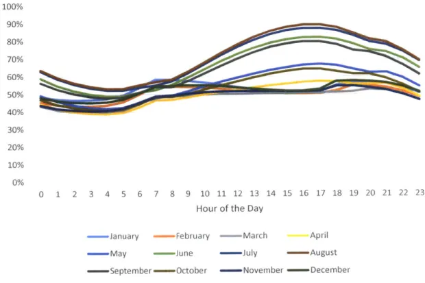
However, deeper analysis of the wind patterns in the Texas market show that there is little correspondence of wind generation and demand. The chart below shows the typical daily load curves for every month of the year, using data from 2012 through 2016, in which 100% is the peak demand hour for that year:

Average Daily Load Curves per Month

100% 90% 80% 70% 60% 50% 40% 30% 20% 10% 0% 0 1 2 3 4 5 6 7 8 9 10 11 12 13 14 15 16 17 18 19 20 21 22 23

Hour of the Day

- January - February - March April

- May - June - July - August

- September - October - November - December

Figure 20 Average Daily Load Curves per Month for the ERCOT System 2012-2016

It is possible to see that the peak demand in Texas is dominated by air conditioning in the warmest months of the year. July and August both have loads on the late afternoon that are on average over

87% the peak for that year, with June and September close behind. The shoulder months have

progressively lower daily peaks, with a small pickup in the winter months for the 7 am and 6 pm average loads.

This behavior shows that about 30% of the peak capacity required in the Texas market would only be used on average 12 hours per day for one third of the year, or about 16% of total hours, utilization rates appropriate for peaking combustion turbine plants. At the same time, no hour of the year averages less than 40% of peak demand, with only a few hours of the night averaging less than 50%, which would represent ideal operation conditions for baseload plants such as nuclear and coal. This analysis, however, is only valid when all the generation sources can be dispatched by the controller. Once wind energy is taken into consideration, it is necessary to consider the net load, i.e., the total load minus the wind energy generation.

ERCOT publishes hourly wind generation on its website. With the total energy generated per hour as a fraction of the total installed nameplate capacity, it is possible to calculate the average capacity

factor for all wind turbines in the system. While the average capacity factor for the period

2012-2016 was 34%, it hourly value varied significantly, from a maximum of 92% to a minimum of 0.1%.

This variation is also dependent on the month of the year and the hour of the day. The chart below presents the average hourly wind capacity factor per month, for the period 2012-2016.

Capacity Factor

Hour of the Day

- January - February - March April

- May - June - July - August

- September - October - November - December

Figure 21 Average Hourly Capacity Factor of Wind Generation Sources per Month for the ERCOT System 2012-2016

Analysis of the data shows that there is a negative correlation between load and wind production. This can be explained due to the fact that the hours of the year with the highest load, which were the afternoons of the months of July and August, are also the periods of the year with the lowest average wind production. The periods with the highest wind energy production, which are from midnight to 4 am on the shoulder months of March, April and May, are also the moments of the year with the smallest load.

Load Duration Curves

% of Hours of the Year

- Load Net Load

Figure 22 Load Duration Curves for 2016

From this data, it is possible to conclude that the addition of wind generation sources at large scale have different effects at different types of thermal power plants. Under the current situation with about 18 GW of nameplate wind capacity installed, the required capacity that operates more than

80% of the hours of the year (one definition of baseload) drops from 32.5 GW to 25.2 GW. At the

same time, the required capacity that operates less than 15% of the hours of the years (the peaking combustion turbine plants) increases from 20.7 GW to 26.0 GW.

This result is compatible with the literature on the topic, as presented in the previous chapter. With higher wind penetration, baseload plants, which are only profitable if they operate a high number of hours, become less necessary. At the same time, the need for fast-response peaking plants increase in order to complement the random wind production.

This effect is dependent on geography, including how large a region can be integrated to share the same generation system. Also, some locations might have wind speeds better correlated with demand. Finally solar will have a different a profile, and in Texas they would be better correlated with peak demand. Analysis of geographic integration and solar production was not part of the scope of this paper.

3.2 Hourly Simulation of the Electric System

In order to better simulate the effects of increased wind penetration in the electric system, this paper will use the available data to study the random distribution of load and wind production. By using a random number generator it is possible obtain representative values for net load.

This simulation was done using data for the ERCOT system for the period 2012-2016. Each month of the year and each hour of the day were analyzed to obtain not only the average load and wind production, but also the distribution.

The image below shows one example of the distributions obtained from the reference to the load, as a fraction of peak load for that year, for 10 am in June.

data, which is in

50.00% 55.00% 60.00% 65.00% 70.00% 75.00%

For each hour per month of the year, a four-parameter beta curve was used to approximate the results, shown in red above. The decision to use the beta curve was due to two factors. First, it is fairly easy to generate random numbers under a beta distribution on MS Excel, a feature that was necessary for fast simulation of 8760 hours per year. The second is that since load was being calculated as a fraction of peak load for a given year (in order to compare data from different years), it was necessary that the distribution was bounded between 0 and 1, which would not be the case under a gamma distribution. Peak load was chosen as the normalization factor because it is the total capacity system operators need to meet. However, any other normalization (such as average load) would generate a similar result.

The same analysis was done to the capacity factor from the wind generation sources for each hour of the day per month, for the period of 2012-2016. The image below shows one example of distribution, for 5 pm on May.

0.00%

20.00%

40.00%

60.00%

80.00%

Figure 24 Histogram of Wind Capacity Factor for 5 pm on May

Similarly, the beta distribution was chosen to approximate the data, since it also needed to be bounded on positive values below 1.

With the parameters for both load and wind capacity factor for all the 288 combination of hour of the day and month, it was possible to simulate the load and net load for the year 2016. The chart

below show the comparison between the original data and the simulated data:

Load Duration Curves

100.0% 90.0% 80.0% 70.0% 60.0% 50.0% 40.0% 30.0% 20.0% 10.0% 0.0% o U, LrA 0 Ln 0 L1n 0 U, 0 LA 0 U, 0) LA 0 Ln 0 Ln 0 Ln 0 LA 0 Ln 0 LA 0. o or*- 6 4 r- 4 4 o6 4 LA o6 c' L-; 6' CN 6. ei ryi 0 6 c r<. 0 4 r-: -4 4 o6 r -4 v- c-i (N~ ('4 r Mo M M~ -<t 1;':T L U) t.0 D f' r-. r- 00 00 00 CA~ 0) 0

- Load - - Simulated Load - Net Load - - Simulated Net Load

As seen above, the simulated load duration curve approximated the load duration curves from the actual data, even if each individual hour deviated. The table below shows the root-mean square error for each fit (to check for accuracy) and the mean error (to check for bias).

Load Wind Capacity Factor

RMSE 9.04E-04 2.86E-03

Mean Error 0.6% -1.5%

Average 57% 34%

Both simulations generated errors and biases that are adequately low for the objective of this paper. Using the simulated data for wind production, it was possible to determine the effects of increased wind penetration on the net load duration curve. As mentioned previously, currently wind capacity is equivalent to 26.6% of yearly peak demand. The model was run with increased wind penetration,

up to five times the current ratio. That means that it is possible that installed wind capacity could be more than 100% peak demand, due to capacity factor constrains.

The chart below presents the net load duration curves for the simulated case. It is important to note that under very high wind penetration net load might be negative. In these cases, for some hours of the year more electricity is produced from wind turbines that demanded in the systems, which would require curtailment of wind turbines.

Net Loads with Increased Wind

100.0% 80.0% 60.0% 40.0% 20.0% 0.0% -40.0% ri1irir4 N r4 M M M I t L n L 1 _r W W 0 -60.0% -80.0%

production is lowest, on afternoon hours in the summer, so the probability of at least on day having very high demand with no wind is significant.

The second conclusion is that while peak demand changes very little, the further down the duration curve the bigger the shift from increase wind capacity. This includes the fact that at wind capacities of about 50% peak load (the wind x2 curve above) there are already hours in the year in which wind electricity production exceeds demand. This behavior would not be true if wind production were constant; in that case, the whole load duration curve would simply shift down at the same rate for all hours.

One possible assumption from interpreting the previous simulation is that each point in the net load duration curve moves linearly with increased wind capacity, though at different rates. That is for example, that the 20-percentile point (the value for load which is only reached on 20% of the hours of the year) will decrease at a lower rate than the 75-percentile point.

To test this assumption and create an equation for the net load duration curve that could be used in the system dynamics model, four points were chosen: peak demand (or zero-percentile, denominated DO), the 20-percentile denominated D20, the 75-percentile denominated D75, and the lowest load of the year (or 100-percentile, denominated DIOO). These points were plotted against wind penetration as a fraction of peak demand. The chart below shows the result.

Shift in the Load Curve as a Function of Wind Penetration

120% 10% -y = -O.0449,x +0.98861,..", 100% .... ---- ----80% 4 -2E 0% y=-0.24046x + 0.4509 -40% -60% m 20% M I% w 20% 40% 6 - 80- 100% 120a 140% -20% - -) -y - -- .4Lnea +0.4877 -40% -60% Y= -0.7426x + 0.3799 -80%

Wind Capacity! Peak Demand

-DO D20 D75 -D100

... Linear (DO)...Linear (D20) ... Linear (D75) - Linear (DiQO)

Figure 27 Shift in Simulated Net Load Curves percentiles, as a function of wind capacity / peak load

This analysis confirms with more clarity the conclusion based on Figure 26, which is that peak net load shifts very little with increased wind penetration, while at the other end of the load duration

---curve values decrease much more rapidly. Also, each percentile decreases linearly at an individual rate. By using these linear approximations, it is possible to create useful net load duration curves for the system dynamics model.

4

DYNAMIC MODELLING OF LONG TERM EFFECTS OF WIND CAPACITY ON

THE ENERGY SYSTEM

The goal of this dynamic model is to simulate what is the effect of increased wind capacity installation on the long term evolution of the electric system in the ERCOT region. The basic hypothesis this model is trying to test is that as wind installation changes the shape of the net load duration curve, the optimal mix of nuclear-coal-natural gas sources change, since those sources have different fix and variable costs. Since the deregulated ERCOT market does not have a central planning authority for investment decisions, this shift is reflected in changes in investment returns for each type of technology, which in turn changes investment rates of private investors.

A secondary hypothesis is that the marginal value of installing new wind resources decrease as wind

share increases, due to negative covariance between generation and prices. As wind capacity increases, a larger fraction of total wind energy production takes place when cheaper marginal producers are determining the price, reducing the average revenue of wind plants. This effects becomes non-linear when wind capacity reaches a scale high enough to cause curtailment, since there starts to be hours in the year when the marginal producer has a marginal cost of zero, and

utilization rates must decrease.

Some assumptions of the model are described below. The first is that the energy capacity consists of five different types of resources, which are wind (suffix Won all variable names), baseload nuclear (suffix B), coal (suffix C), intermediate combined cycle natural gas (suffix M), and combustion turbine peaking natural gas (suffix P).

The second is that due to the competitive energy market nature of the ERCOT system, the marginal cost of the marginal producer at every hour determines the energy price at that hour. Due to its lower marginal cost, nuclear always produces before any coal plant, which always produce before

NGCC, and so on. One exception to this assumption is for peaking plants. Since they are required to

meet peak load, it is assumed that if there isn't excess peaking capacity prices can go above marginal cost (this is further detailed below).

The third assumption is that while variable, and fix operating costs remain constant over time, specific construction costs (expressed in $/MW) decrease over time. The reason for this is that for

The fourth assumption is that the basic shape of the load duration curve does not change over time, and that net load is only a function of installed wind capacity as a fraction of peak demand. For this reason, changes such as storage and demand side response technologies were not considered. Yearly peak load was simulated as a constant exponential growth rate, which is the projection from ERCOT for the next decade. [16]

Finally, though the stock of each capacity and peak demand are expressed in MW, all the model uses values for capacity is the ratio of that capacity to the peak demand, in percentage points. This is due to assure that the model can be easily scaled to different situations. This should not affect the accuracy of the model, since all the effects such as displacement of the net load curve and average revenue are a function of the ratios of the different sources, instead of the nominal values. Therefore, when describing the model as having, for example, a wind capacity of W, it should be understood that W is the nominal installed capacity, in MW, divided by the expected peak load for that year, also in MW. Similarly, period durations are expressed as fraction of hours per year. For example, if the model says that nuclear baseload determines the price 20% of the time, it means 20% times 24*365 hours per year for a normal year.

For this paper, the description of the model will be divided in the following parts:

" Calculation of how much energy each source would produce in a given net load duration curve condition, including how many hours a week each different source determines the

price by being the marginal source.

* Financial calculation of average revenue per MWh for each generation source and levelized cost of electricity.

" Definition of investment rates, which in turn determine the stock for each type of energy source.

From a very high level perspective, the essential dynamic on this market is that the present mix of different generation sources affect the profitability of the rest, which in turn affect the investment rate, which in the long term affects the generation mix.

Generation Mix

In the Energy

Investment

Market

I

Rates

Shape of Net

Load Curve

Revenue and

Costs for Each

Source

Each section below details the interactions.

4.1 Definition of Utilization Rates for Each Generation Source

This section will describe how the system dynamics model calculates how much energy is being produced from each energy source, and for each energy source how much is being produced when another is determining the price.

As explained in the previous sessions, variable renewable sources such as wind can be considered as negative load. Since they can't be dispatched, they need to be modeled as random, though predictable, generation, which is similar to how demand is modeled.

In the model below, the total load curve is determined as being formed by four points: LO, 120, L75, and L100. Those points represent the peak load, 20-percentile, 75-percentile, and minimum load, respectively. They are also considered to be constant, in accordance to assumption four above. The net load duration curve shape is determined as a function of the wind capacity, and it is formed

by four points DO, D20, D75, and D100. Those points represent peak net load, 20-percentile,

75-percentile, and minimum net load, respectively. It is important to note that net load might be negative; in those cases it is assumed there is wind curtailment, which means wind turbines do not produce as much energy as they could.

The capacities of each of the five types of sources are defined as W, B, C, M, and P, for wind, baseload nuclear, coal, intermediate NGCC, and peaking NGCT, respectively. Those capacities determine four important periods. Variable hO is the percentile at which net load crosses zero. Variable hb is the percentile at which capacity B crosses the net load curve, with similar definitions for hc and capacity C, and hm and capacity M.

The drawing below shows a graphical representation of these variables:

L0

DO

P L20

-J L75

4-dimensionless ratios, the result is also a 4-dimensionless values, which need to be multiplied by peak demand in MW and hours per year to result in MWh/year.

Since the load curve was simplified as a sum of three straight lines, it is possible to calculate the area below as simply a sum of discrete rectangles, triangles and trapezoids. The figure below shows an example of how it would be calculated. The energy produced from baseload nuclear would be the area below both the line B and the net load curve. For coal, it would be the area between B and B+C, and below the net load curve, and so on. All the area between the total load and net load curves is equivalent to the energy from wind sources, except when net load goes negative.

P

0--- --- ---.-.-.---. . . . ..-- --

--hm---b---.

HC- -s -%---H--s

gn

hoursbetwen h andhb, ucler beweenHur (nd of, totale ours) pic nal ousaov Thepgcure 30shw aGraphical representation of thesleeg erbenes:suc

Anothr imortat inormaton i howmuchenery is rodued wen-agivenenery-sorce-s-th marginal~~~~~~~~ prdue and- set th price- in-heenrg-cmptitvemake.-n-hi-cotetevrysorc

with~~~~~~~~~~~~~~- a-- loe marina cos prdue-bfreon-it--hghr-Frths- esopekigplns-e the riceon te hors fom zro t hmintemedate GCC n hors fom h-to-c,-cal-pantsfor

hour beteen c an hb nucear etwen hbandho, hilewindsetsprie onall-oursabov-h-Th pitreblo-hosagrpiclrersettono-tee-aials

P 0 GM CL 0. C 0 B hm hc hb hO

Hours (% of total Hours)

Figure 31 Energy produced when each source determines the price

Combining the information from both graphs, it is possible to then determine the average revenue for each energy source. The utilization rate, which is the energy produced divided by total capacity (also known as capacity factor), determines the levelized cost of electricity. Both those determine the investment rates. These effects will be detailed in the following sessions.

Variable _{Type Unit} Description Name Ratio of wind W Variable % of PD capacity to peak demand Ratio of baseload B Variable % of PD capacity to peak demand Ratio of coal C Variable % of PD capacity to peak demand Ratio of intermediate M Variable % of PD capacit capacity to peak demand Ratio of peak P Variable % of PD capacity to peak demand

DO Variable % of PD Max Net Load

D20 Variable % of PD 20-percentile net load D75 Variable % of PD 75-percentile net load Minimum Net D100 Variable % of PD Load Peak Load

LO Variable _{% of PD without Wind}

20-percentile

L20 Variable % of PD load without

Wind 75-percentile L75 Variable % of PD Minimum Load L100 Variable % of PD Total energy % of demand in an TD Variable PD*H year as a fraction of PD * H Total energy % of net-demand in TND Variable an year as a fraction of PD H Percentile where the Net

Load Curve hb Variable % of H Cre crosses baseload capacity Percentile where the Net

hc Variable % of H Load Curve

crosses coal capacity

Equation

Wind Capacity / Peak Deman

Nuclear Baseload Capacity / Peak Capacity

Coal Capacity/Peak Demand

Intermediate Capacity / Peak Demand

Peak Capacity / Peak Demand

-0.0141 * W + 0.9639 -0.1979 * W + 0.649 -0.4514 * W + 0.4883 -0.7382* W + 0.381 0.649 0.4883 0.381 ((L0+L20)/2)*0.2+((L20+L75)/2)*(0.75-0.2)+((L75+L100)/2)*(1-0.75) ((DO+D20)/2)*0.2+((D20+MAX(D75,0))/2)*(MIN(0.75 ,HO)- 0.2)+((MAX(0,D75)+MAX(0,D100))/2)*(MIN(HO,1)-MIN(HO,0.75))

IF THEN ELSE( B<D100,1,IF THEN ELSE( B<D75,0.75+0.25*(B-D75)/(D100-D75),IF THEN ELSE(B<D20,0.2+0.55*(B-D20)/(D75-D20),IF THEN

ELSE(B<D,0.2*(B-DO)/(D20-DO),0)))) IF THEN ELSE( (B+C)<D100,1,IF THEN ELSE( (B+C)<D75,0.75+0.25*((B+C)-D75)/(DOO-D75), IF THEN ELSE(

(B+C)<D20,0.2+0.55*((B+C)-D20)/(D75-D20),IF THEN ELSE( (B+C)<DO,0.2*((B+C)-DO)/(D20-DO),0))))

Type Unit Description Percentile where the Net

hm Variable %of H LoadCurve

crosses intermediate

capacity Percentile where the Net

hO Variable %of H Load Curve

crosses zero demand Yearly Energy

% of Produced at

EPP Variable PD*H Peak Prices as

a fraction of PD *H Yearly Energy Produced at Variable % of Intermediate EMP _PD*H Prices as a fraction of PD * H Yearly Energy % of Produced at

ECP Variable PD*H Coal Prices as a

fraction of PD* H Variable % of PD*H % of Variable _PD*H Variable % of PD*H Yearly Energy Produced at Baseload Prices as a fraction of PD * H Yearly Energy Produced at Wind Prices as a fraction of PD * H Yearly Energy Produced from non Wind sources at Peak Prices as a Equation

IF THEN ELSE( ((B+C+M))<D100,1,F THEN ELSE(

((B+C+M))<D75,0.75+0.25*(( (B+C+M))-D75)/(D100-D75),IF THEN ELSE( ((B+C+M))<D20,0.2+0.55*(

((B+C+M))-D20)/(D75-D20),IF THEN ELSE( ((B+C+M))<DO,0.2*(((B+C+M))-DO)/(D20-DO),O))))

IF THEN ELSE(D100<OIF THEN ELSE(D75>0,1+((-

D100/(D75-D1OO))*(-0.25)),0.75+(0.2-0.75)*(D75)/(D75-D20)),1)

((LO+MAX(LHML20))/2)*MIN(HMO.2)+IF THEN ELSE( HM>0.2, ((L20+ MAX(LHM,L75))/2)

*(MIN(o.75,HM)-0.2),o)+F THEN ELSE( HM>0.75,

((L75+MAX(LHM,O,L1OO))/2)*(MIN(HM,hO,1)-0.75),0)

((LO+MAX(LHC,L20))/2)*MIN(HC,0.2)+IF THEN ELSE(

HC>0.2,((L20+MAX(LHC,L75))/2)*(MIN(O.75,HC)-0.2),O)+IF THEN

ELSE(HC>0.75,((L75+MAX(LHC,,L100))/2)*(MIN(HC, hO,1)-0.75),O)-EPP

((LO+MAX(LHB,L20))/2)*MIN(HB,0.2)+IF THEN ELSE(

HB>0.2, ((L20+MAX(LHB,L75))/2)

*(MIN(O.75,HB)-0.2),0) +IF THEN ELSE( HB>0.75,

((L75+MAX(LHB,,L100))/2)* (MIN(HB,hO,1)-0.75),O)-EPP-EMP ((LO+L20)/2)*0.2+((L20+MAX(LHO,L75))/2)*(MIN(O.7 5,hO)-0.2)+((L75+MAX(LHO,L1OO))/2)*(MIN(hO,1)-0.75)-EMP-EPP-ECP TD-EMP-EPP-EBP-ECP ((DO+MAX((B+C+M),D20))/2)*MIN(HM,0.2)+F THEN ELSE( HM>0.2, ((D20+ MAX((B+C+M), D75))/2)

*(MIN(o.75,HM)-0.2),o) + IF THEN ELSE( HM>0.75,

((D75+MAX((B+C+M), 0,D1OO))/2)*(MIN(HM,hO,1)-Variable Name EBP EWP EPP-nonWind

Variable Type

Name Unit Description

Prices as a fraction of PD * H Equation ((D75+MAX(BODWN-))/2) *(MIN(HBhO,1)0.75), 0)-EPPNONWIND-EMPNONWIND Yearly Energy Produced from % of non Wind

EBP_nonWind Variable PD*H sources ats

Baseload Prices as a fraction of PD * H Yearly Energy Produced By BE Variable % of Baseload PD*H Sources as a fraction of PD * H Yearly Energy % of Produced By

CE Variable PD*H Coal Sources as

a fraction of PD *H Yearly Energy Produced By % of Intermediate PD*H Sources as a fraction of PD * H Yearly Energy %f Produced By

PE Variable Peak Sources

as a fraction of

PD * H Yearly Energy Produced from

WE Variable Po* Wind as a

fraction of PD *

H

Capacity Factor

CFB Variable % of Baseload

Sources

CFC Variable % Capacity Factor

CFC Vriabe % f Coal Sources

Capacity Factor CFM Variable % of Intemediate Sources Capacity Factor CFP Variable % of Peak Sources Capacity Factor CFW Variable % of Wind Sources Auxiliary variable, total

Lho Variable %of PD load at

percentile hO TND-EMPNONWIND-EPPNONWIND-ECPNONWIND EBPNONWIND+B*HB (ECPNONWIND-B*(HB-HC))+C*HC EMPNONWIND-(B+C)*(HC-HM)+HM*M EPPNONWIND-HM*((B+C+M)) TD -TND BE/B CE / C ME/M PE/P WE/W

IF THEN ELSE( H0>0.75,L100+(HO-1)*(L100-L75)/0.25, IF THEN ELSE(

Variable _{Type Unit Description} Name Auxiliary variable, total Lhb Variable % of PD load at percentile hb Auxiliary variable, total Lhc Variable % of PD adbat percentile hc Auxiliary variable, totalI Lhm Variable % of PD loda percentile hm Equation

IF THEN ELSE(

HB>0.75,L1OO+(HB-1)*(L1OO-L75)/0.25, IF THEN ELSE(

HB>0.2,L75+(HB-0.75)*(L75-L20)/0.55,L20+(HB-0.2)*(L20-LO)/0.2))

IF THEN ELSE(HC>0.75,L1OO+(HC-1)*(L1OO-L75)/0.25,IF THEN

ELSE(HC>0.2,L75+(HC-0.75)*(L75-L20)/0.55,L20+(HC-0.2)*(L20-LO)/0.2)) IF THEN ELSE(

HM>0.75,L1OO+(HM-1)*(L1OO-L75)/0.25, IF THEN ELSE( HM>0.2,

L75+(HM-0.75)*(L75-L20)/0.55,L20+(HM-0.2)*(L20-LO)/0.2))

4.2 Financial Calculations for the Energy Model

The financial calculations on the energy model are divided in two parts, the cost calculator and the revenue calculator.

For the cost, the metric used was levelized cost of electricity. This metric of $ per MWh considers three different main costs of energy: the capital cost due to construction and asset depreciation, the fixed operating cost, and the marginal cost (which include both fuel cost and variable operating cost). It can be understood as the price of electricity that would drive the net present value of an energy investment to zero.[19]

For all metrics, the source for data regarding new investments in the United States was the information from the Department of Energy.[201

4.2.1 Capital Costs

The capital cost fraction of the levelized cost of electricity include both the financing cost of installing a new plant and the depreciation cost associated with existing plants.

The basic formulation of the capital cost per MWh for technology k is the following: [19] SCk * CRF

CFk* 8760

Where CC is expressed in $/MWh, SC is the specific construction cost expressed in $/MW, CRF is the capital recovery factor (described below), CF is the capacity factor (or utilization rate) of the technology expressed in percentage points, and 8760 is the total number of hours in one year.