Effect of Magnetic Seed Fields on Lyman Alpha
Emission from Distant Quasars
by
Sruthi Annapoorny Narayanan
Submitted to the Department of Physics
in partial fulfillment of the requirements for the degree of
ASSAC INSTITUTE OFTECHNOLOGY
JUL 0 72016
LIBRARIES
ARCHIVES
Bachelor of Science in Physics
at the
MASSACHUSETTS INSTITUTE OF TECHNOLOGY
June 2016
@
Massachusetts Institute of Technology 2016. All rights reserved.
Author
...
Signature redacted
Department of Physics
May 6, 2016
Certified by....
Signature redacted
Mark Vogelsberger
Assistant Professor of Physics
Thesis Supervisor
Accepted by...
Signature redacted
Nergis Mavalvala
Associate Department Head of Physics, Senior Thesis Coordinator
Effect of Magnetic Seed Fields on Lyman Alpha Emission
from Distant Quasars
by
Sruthi Annapoorny Narayanan
Submitted to the Department of Physics on May 6, 2016, in partial fulfillment of the
requirements for the degree of Bachelor of Science in Physics
Abstract
There are indications that weak magnetic fields originating in the early Universe and magnified via magnetohydrodynamic (MHD) processes could cause perturba-tions in the thermodynamic state of the gas in the intergalactic medium which affect the Lyman-Alpha spectrum we observe. In this work we investigate to what extent the properties of the Lyman-Alpha forest are sensitive to the presence of large-scale cosmological magnetic fields as a function of the seed field intensity. To do so, we develop and use a series of numerical tools to analyze previously constructed cosmo-logical MHD simulations that include state-of-the-art implementation of the relevant physical processes for galaxy formation. The inclusion of these physical mechanisms is crucial to get the level of magnetic field amplification currently observed in the struc-tures that populate our Universe. With these tools we isolate characteristics, namely the Flux Probability Density Function and the Power Spectrum, of the Lyman-Alpha forest that are sensitive to the magnetic field strength. We then examine the impli-cations of our results.
Thesis Supervisor: Mark Vogelsberger Title: Assistant Professor of Physics
Acknowledgments
First and foremost I would like to acknowledge Federico Marinacci who has provided so much assistance in the writing of this thesis. I would like to thank him for patiently reading every draft and giving me thorough comments as well as helping me to learn and understand all the integral physics for this project. His help has been invaluable. I would also like to thank Professor Vogelsberger for his guidance and useful discussion.
My overall experience at MIT has been shaped by my friends. In particular Elise
Newman, Francisco Machado, Will Conway and Nick Rivera have made my time here especially fruitful. They have helped me a considerable amount in understanding this project. I would also like to thank Evan Zayas for his help and motivation when writing my thesis because everyone needs that one person who they can complain to all the time and who can also help them with physics.
Lastly I want to express my gratitude and love to my parents who have been with me through countless endeavors over the past four years and constantly give me a reason to not give up.
Contents
1 Introduction 13
2 The Ly-a Forest 19
2.1 Proposed Effect of Magnetic Fields . . . . 23
3 Simulation Details 25
3.1 Analyzing Simulation Output . . . . 28 3.1.1 Choosing a Random Line of Sight . . . . 28 3.1.2 Interpolation along line of sight . . . . 29
4 Computing Ly-a Spectrum 31
4.1 Error Estimation Methods . . . . 33
4.1.1 Bootstrap Method . . . . 33
4.1.2 Jackknife Method . . . . 34
5 Results and Discussion 36
5.1 Flux Probability Density Function . . . . 42
5.2 Power Spectrum . . . . 44
6 Conclusions and Summary 46
A Cosmology 48
A.1 ACDM Cosmology . . . . 48
A.1.1 A Simple Example . . . . 49 A.2 Adiabatic Heating and Cooling . . . . 50
B Astrophysics 52 B.1 Reionization . . . ... .. . . .. .... .... . . . .. 52
List of Figures
1-1 The cosmological epochs . . . . 15
1-2 Visualization of the magnetic field strength in the simulation box at redshifts z = 4.1 and z = 0 . . . . 17
2-1 Example star absorption spectrum and quasar emission spectrum . . 20
2-2 Toy model of quasar emission spectrum . . . . 21
2-3 Variation in gas density with magnetic field . . . . 23
3-1 Simulation box with random line of sight and interpolation cylinder 29 3-2 Example of tesselation of two dimensional simplices . . . . 30
5-1 Spectra as a function of distance for B = 10-12 G and z = 2.0 . . . . 37
5-2 Column density of neutral hydrogen for B = 10-12 G . . . . 37
5-3 Spectra as a function of distance for B = 10-12 G and z = 2.5,3.0 . 39 5-4 Spectra as a function of distance for B = 5 x 10-' G and z = 2.0 . 40 5-5 Column density of neutral hydrogen for B = 5 x 10-' G . . . . 40
5-6 Spectra as a function of distance for B = {10-12, 10-11, 10-10, 10-9, 5 x 10⁻⁹, 10-8} G and z = 2.0 . . . . 41
5-7 Magnetic field variation of the Flux PDF for z = 2.0 . . . . 43
5-8 Magnetic field variation of the power spectrum for z = 2.0 . . . . 45
List of Tables
3.1 Properties of the performed simulations . . . . 26
Chapter 1
Introduction
Magnetic fields are an essential component in many astrophysical phenomena at all mass and length scales ranging from stars to galaxy clusters and possibly extend-ing even to the intergalactic medium (Govoni and Feretti [2004]). The rotation of compact objects, like supermassive black holes, affects the magnetic fields lines by "twisting" and "tangling" them.' Twists and tangles can produce highly localized fields with the potential to generate relativistic jets that propagate into the intra-cluster medium (Blandford and Znajek [1977]) which can then affect the accretion on compact objects like neutron stars and supermassive black holes (Balbus [2003]). Additionally magnetic fields affect the propagation of relativistic particles like cosmic rays which then have an effect on other observable astrophysical processes (Kotera and Olinto [2011]).
At the level of galaxies, the magnetic fields allow for the production of synchrotron radiation seen in disc galaxies (Beck and Krause [2005]) and in some active galactic nuclei (AGN) (Urry and Padovani [1995]). On smaller scales (smaller than galaxies and clusters) magnetic fields provide magnetic pressure that acts along with thermal pressure against gravity in the interstellar medium (ISM) and potentially the inter-galactic medium (IGM) (Boulares and Cox [1990]). The study of the origin and the
'For example, twisting and tangling of magnetic fields is what causes the polarity of the Earth's magnetic field to switch.
evolution of these fields is therefore a key aspect in our understanding of the Uni-verse. However, it is not yet clear from a theoretical perspective how magnetic fields were generated in the early Universe and whether these fields affected the structures that developed later on. There are indications that pre-existing magnetic fields were magnified by dynamical processes in our Universe but we still do not understand the origins of this supposed seed field (Widrow et al. [2011]).
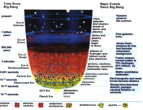
One proposed model suggests a cosmological origin of the seed, which means it was generated via inflationary processes. This could have occurred due to phase tran-sitions. It is postulated that in the early Universe, phase transitions were present that changed the nature of particles and fields. For example, electroweak symmetry breaking marked the transition from a high-energy regime in which the W and Z bosons and the photon were effectively massless and interchangeable to one in which the W and Z bosons were heavy while the photon remained massless. This transi-tion coincided with the increased relevance of electromagnetism and the weak nuclear force (Widrow et al. [2011]). Transitions like this one had potential to generate strong magnetic fields because they involved the release of a lot of energy. In Figure 1-1 we show a time table of the cosmological epochs in the early universe that could have contributed to the production of a seed field.
A non-inflationary process that could have contributed to the production of a seed
field is the Biermann battery mechanism proposed by L. Biermann in 1950 that can occur simultaneously with cosmological shocks (Ryu et al. [1998]) or during cosmic reionization (Gnedin [2000]). It is then proposed that these seed fields were amplified
by turbulent processes or galactic dynamos (baryons collapse into dark matter haloes
that assemble structures in our Universe.)
Another class of models suggests that the magnetic fields were produced by stars in protogalaxies and then later ejected outwards, conceivably by the Biermann mech-anism mentioned above (Schoeffler et al. [2016]). Whereas we seem to have many
Time Since
Big Bang Major EventsSince Big Bang
present
stars,
Era of galaxies
Gataxie! and clusters
Galaie e (made of
I billion sma
years oms and
E ra of Jstars
Atoms bagin
500,000 form)
years plasma of
Er. - hydrogen and
NuE0e helium nuclei
Cie nplus electrons
3 minutes.
protons. neutrons
Era ol - ~ electrons. neutrinos
Nucleosynthesis (antimatter rare)
0.001 seconds
Omentary partlcles
Particle Era e e * O
, ltmattor
10 seconds a g common) El.
Electroweak Ern - ele Io
13- Pa'ticles Sti
10 seconds dis
GUT Ern elementary ca
104 seconds particles un Planck Era ???? Humans observe the cosmos. First galaxies form. Atoms form;
photons fly free and become microwave background, Fusion ceases; normal matter is 75% hydrogen. 25% helium, by mass. Matter annihilates antimatter.
ctromagnetic and weak
ces become distinct.
rong force becomes tinct, perhaps using inflation of iverse.
neutron electron antiproton - a q
proton neutrino antineutron n rou k Copyrghlt V Addisna Wesliy
Figure 1-1: The inflationary epoch was from 10-36 to 10-32 seconds and is where the
universe underwent a rapid exponential expansion. Reheating came after this and the quantum chromodynamic quark-gluon-plasma period lasted until hadron forma-tion. The hadron epoch lasted from 106 to 1 second. At later times the period of relativistic and classical plasma sets on. Here seed magnetic fields can be gen-erated from thermal background electrodynamic fluctuations if thermal anisotropies or beams can exist in this regime. (From http://ircamera.as.arizona.edu/NatScil02/ lectures/eraplanck.htm.)
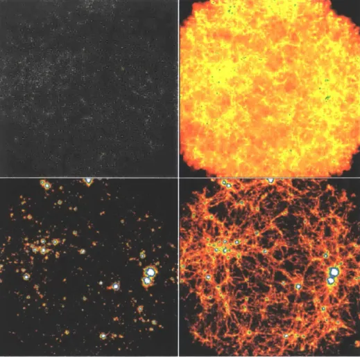
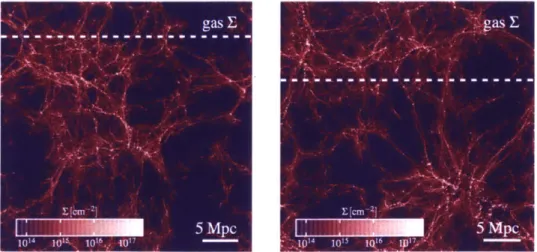
models for the theoretical origin of the seed field, as with any experimental science we need observational evidence to validate our claims. Intuitively if we could measure the field at various points in space, in particular in low density environments, we could deduce information about the influences of magnetic fields on cosmological structures. In Figure 1-2 from (Donnert et al. [2009]) we look at how the magnetic field strength varies in regions of different redshifts. At high redshifts (close to the beginning of our Universe's time scale) there was not a lot of structure (like galaxies) so the gas present in space was more dense. As we moved forward in time various forces such as gravitational interactions and magnetic fields shaped the gas and formed structures. The gas left between the structures was appropriately called the Intergalactic Medium (IGM) and became less dense because of the expansion of the Universe.
We observe that as we evolve to z = 0 the magnetic field distribution becomes more
clustered as opposed to homogeneous. This figure is relevant because it shows us the difference between using the initial conditions of instantaneous seeding and a homo-geneous seed field. We observe that the low density regions are potentially very useful to understand which of these two scenarios are correct because of the differences in the magnetic field distribution as mentioned above. Whereas we have simulations that can evolve the magnetic field strength, it is hard to observe these magnetic fields because their expected field strengths are < 1 nG compared to galactic magnetic fields
that are about 10 pG (Marinacci and Vogelsberger [2015]). Though direct detection methods are improving (Beck [2007]) we can also gain crucial insights by analyzing the effects of magnetic fields in cosmological simulations on quantities that can be directly compared to the available observational constraints. For the purposes of this work and for simplicity in the generation of initial conditions we focus on the homo-geneous seed field scenario.
In this work, we will use methods of indirect detection of magnetic fields. Detailed in-formation about the large-scale distribution of neutral gas in the Universe can come from observations of the so-called Lyman-a (Ly-a) forest. The Ly-a forest is the
Figure 1-2: Every image shows a region of a linear size of 204 Mpc/(1
+
z). The upper left panel shows the magnetic field due to instantaneous seeding with maximum field strengths of ~ 5 nG. The upper right shows a simulation with homogeneous cosmological magnetic seed field. The field strength reaches values of up to ~ 10 nG. The lower two panels show both simulations evolved to z = 0. Adapted from (Donnert et al. [2009]).spectrum of absorption lines that originates when the ultraviolet light coming from distant quasars travels through the intergalactic medium and is absorbed by clouds of cold gas intervening between the quasar and the observer on Earth. We discuss this feature in more detail in Chapter 2. Most of the absorption occurs at frequen-cies of the Ly-a transition as that frequency corresponds to the energy that excites electrons in neutral hydrogen. Due to the expansion of the Universe, the frequency of the transition is redshifted according to the observer's distance. In practice, the redshift of the transition is directly proportional to the distance of the intervening cloud from the observer. This relationship allows us to probe the conditions of the gas in the intergalactic medium in a very large range of distances and times during the evolution of the Universe.
There are indications that weak magnetic fields originating in the early Universe and magnified via magnetohydrodynamic (MHD) processes, as previously discussed, could cause density perturbations which affect the Ly-a spectrum we observe. In this work we investigate to what extent the properties of the Ly-a forest are sensitive to the presence of large-scale cosmological magnetic fields as a function of the field intensity. This will hopefully help us understand the extent to which fluctuations of the Ly-a spectrum depend on magnetic field strength.
We begin this work with a detailed discussion of the Ly-a forest and its possible response to magnetic seed field strength in Chapter 2. The numerical tools we use for our analysis are discussed in detail in Chapters 3 and 4. With these tools we will attempt to isolate characteristics of the Ly-a forest that are sensitive to the magnetic field strength. This will hopefully aid in the interpretation of the wealth of existing Ly-a forest observations as we discuss in Chapter 5. We draw conclusions and provide insight for further study in Chapter 6. Relevant topics in cosmology and astrophysics are discussed in Appendices A and B respectively.
Chapter 2
The Ly-a Forest
An active galactic nucleus (AGN) is a very compact region at the center of a galaxy that has a higher than normal luminosity. The radiation given off by an AGN is most commonly believed to be a result of accretion of mass by a supermassive black hole at the center of the associated galaxy. A quasar is a type of AGN whose galaxy axis (the axis going through it's galactic center) points toward the Earth. As a result we see a high amount of emission from them which is why they appear as some of the most energetic AGNs. If we were to look at a picture of the sky, the naked eye would not be able to distinguish a quasar from a star because they look the same. However if we were to look at their spectra, how they spread light, as in Figure 2-1 we notice that stars are characterized by an absorption spectrum and quasars by an emission spectrum with different characteristics. We also notice that the Ly-a peak at the far left of the quasar emission spectrum is the peak with the highest amplitude. Since quasars produce a high level of Ly-a emisson, in this work we use quasars as our primary source and concern ourselves with the resulting emission spectrum.
The Ly-a forest is caused by the absorption of Ly-a photons by neutral hydrogen atoms along a line of sight to a distant source, in our case a quasar. Originally the forest was described using clouds of gas by E.M. Lynds in 1971. These clouds were supposed to be similar to clouds in the interstellar medium. The velocity widths (absorption as a function of the velocity of the cloud) of the absorption spectrum
RA -146,91375, DEC- 0.64448. MJD-51630, PNote- 266, Fiter- 15P
S S1 H kMg No ; Nll !
P) & fJil' Coll
11 0111 61HI donl
40D 5 000~ 6 000 0 (1700 800 an0 4,,q( sa
Figure 2-1: In the left panel we show the absorption spectrum from a star (from http://cas.sdss.org/dr3/en/proj/advanced/spectraltypes/lines.asp) which is notably different from the emission spectrum of a quasar though to the naked eye both are indistinguishable. The right panel shows an example emission spectrum from a quasar (from http://www.astrosurf.com/buil/galaxies/spectra.html). On the horizontal axis we have the wavelength and on the vertical axis is the radiation flux density. We observe that there is more emission at higher wavelengths which corresponds to higher redshift.
lines were primarily attributed to the thermal motion of the absorbing atoms. A toy model of this spectrum is shown in Figure 2-2. There has since been a continuing effort to understand the origin of the Ly-a forest by modeling it through numerical hy-drodynamic simulations of Cold Dark Matter (CDM) cosmologies (Dav6 et al. [19971).
Since the Ly-a forest is affected by the gas present in the IGM, it is useful to un-derstand the factors that affect the IGM gas and temperature distribution. Analytic results (Hui and Gnedin [1997]) suggest that the evolution of the temperature of the IGM is as follows
dT 2T [2T d6 T dm 2 dQ (2.1)
dz 1+ Z 3(1+6) dz m dz 3kBnb dz
where 6 and H(z) depend on the cosmology and the gas overdensity 1 + 6 = p/p,
m is the mean particle mass (total mass divided by the number of particles), kB is
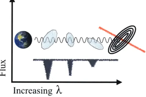
A
Increasing
X,
Figure 2-2: We model light (wavy line) being emitted from a quasar and following a path to Earth (the observer.) Along the way the light passes through "clouds" of neutral hydrogen. The corresponding absorption spectrum is then roughly shown under the pathway of the light.
unit volume that comes from the ambient radiation field. In Equation 2.1 the first two terms describe heating and cooling due to adiabatic processes (see Appendix A). The third term is due to the change in the ionization fraction (see Appendix B). The fourth term is a result of heat transfer from the ambient radiation. Hydrogen reionization produces one photoelectron per hydrogen atom and heats the IGM. Then adiabatic cooling brings the overall temperature down. The regions with higher densities of neutral hydrogen remain hotter than other regions because they have higher heating rates (Peeples et al. [2010]). For a redshift z the equation of state (relation between temperature and density) is well approximated by a power law
T(z) = To(z)(1 + 6)a(z). (2.2)
Semi-analytic methods are used (Hui and Gnedin [1997]) in conjunction with simu-lations to justify the above power law approximation. Previous results have found that after reionization (at a given redshift) To ~ 104K and a ~ 0.6 (Hui and Gnedin
[1997]).
In our analysis of the Ly-a forest we are primarily concerned with a quantity called the optical depth -rHI, how much absorption occurs when light travels through an absorbing medium. This quantity is related to both the temperature and density by a power law as we discuss explicitly in Chapter 4 which implies that the Ly-a forest spectrum would be affected by both temperature and density fluctuations. Hence there is an implicit relationship between the optical depth and the equation of state. An analysis of the optical depth will allow us to determine properties of the gas density and then using the equation of state we can relate density fluctuations to temperature fluctuations.
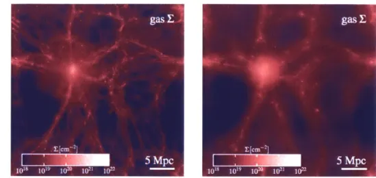
Figure 2-3: We plot the column density (mass per unit area) in a 25 Mpc box for a magnetic field of 10-11 G on the left and 10-' G on the right. We observe that the column density noticeably changes with a variation in magnetic field.
2.1
Proposed Effect of Magnetic Fields
Discussions of the effects of magnetic fields on the Ly-a forest are not prevalent in the previous literature about Ly-a absorption. In this work, the main goal is to determine the extent of the influence that the magnetic field strength has on the Ly-a Ly-absorption. As mentioned in ChLy-apter 1, mLy-agnetic fields Ly-affect the IGM by exerting a force via magnetic pressure that counters gravity. The magnetic pressure is given by
B2
PB = . (2.3)
8 r
where B is the magnetic field strength. To understand why the magnetic pressure can change the thermodynamic state of the gas, consider an ideal gas in a gravitational field. Gravitational interactions keep the gas together and thermal pressure results in an expansion force countering gravity. Adding a magnetic pressure results in the system requiring less thermal pressure to maintain the same equilibrium since the two pressures are additive. Thermal pressure is pressure due to the movement of the atoms in a gas and is given by
where T is the temperature, p is the density and p is the mean molecular weight of particles of mass mp. We can simplify this by saying P = np is the total number particle density since pm, is the average mass of the particles that compose the gas
so
PT = npkBT (2.5)
which is a familiar relation for ideal gases. This quantity depends on the temperature and density of the gas so changes in thermal pressure can result in changes to the density of the gas and therefore changes in Ly-a absorption. Additionally changes in the density of the gas can cause changes in the temperature via the equation of state in Equation 2.2.
We look at an example of this effect in Figure 2-3. Both panels are plots of the gas column density in simulated 25 h-'Mpc cosmological boxes as per (Marinacci et al. [2015]). We discuss the simulation used to produce these plots in Chapter 3.
All simulation parameters were kept the same except for the initial magnetic seed
field intensity. The left panel uses a magnetic field strength of 10-11 G and the right panel 10-8 G. There appears to be a noticeable difference in the structure of the gas. If we considered a line parallel to the x-axis and through the center of the box then the absorption as a function of distance would be different for each box as the density distribution of gas is not the same. This difference demonstrates the effect of mag-netic field strength on the density distribution of gas and hence of neutral hydrogen. In our analysis we will investigate this connection in more detail. In particular our aim is to find whether statistical properties of the Ly-a forest (such as the Flux PDF and Power Spectrum) are affected by the presence of a cosmological magnetic seed field and if so to determine the magnetic seed field strength needed for this effect to be visible.
Chapter 3
Simulation Details
In this work we use results from numerical cosmological simulations as discussed in a recent paper (Marinacci and Vogelsberger [2015]). The simulations used for this project use a cosmological box of size 25 h-'Mpc. From here on h is the Hubble parameter, a normalized value of the Hubble constant given by
h = km/s/Mpc. (3.1)
100
The total particle number in our chosen box is 2 x 2563. This provides a measure of the resolution of our simulation because the number of particles determines the number of data points, so the more particles the higher the density of data points and hence the higher the resolution of our simulation. We tabulate in Table 3.1 the details of each performed run as in Table 1 in (Marinacci and Vogelsberger [2015]).
The cosmological parameters used are in accordance with an analysis of Planck data from (Spergel et al. [2015]). We assume a ACDM cosmology (refer to Appendix A) with parameters
QM = 0.302, Qr = 0.04751, QDE = 0.698
Simulation Ntot MDM Mgas f Bo (DM + cells) (10' h-MO) (105 h-'M®) (h-lkpc) (G) box-256-fp-le12 2 x 2563 1.64 x 10² 3.07 x 101 1.2 (0, 0,10-12) box-256-fp-lell 2 x 2563 1.64 x 10² 3.07 x 101 1.2 (0, 0,10-") box-256-fp-lelO 2 x 2563 1.64 x 10² 3.07 x 101 1.2 (0, 0, 10-10) box-256-fp-1e9 2 x 2563 1.64 x 10² 3.07 x 101 1.2 (0,0, 10-9) box-256-fp-5e9 2 x 2563 1.64 x 10² 3.07 x 101 1.2 (0, 0, 5 x 10⁻⁹) box-256-fp-le8 2 x 2563 1.64 x 10² 3.07 x 101 1.2 (0,0,10-8)
Table 3.1: Columns give (from left to right): simulation name, total number of dark matter particles plus gas cells, mass resolution in the dark matter component, mass resolution in the gas component, maximum physical gravitational softening (reached at z = 1), and initial (comoving) seed magnetic field. Adapted from (Marinacci and
Vogelsberger [2015]).
In addition to the parameters given in Appendix A, n, is the exponent of the power law that the primordial density perturbation follows where n" = -1 corresponds to a
scale invariant power spectrum (all the fluctuations have the same power at all length scales) and is the value predicted by inflationary models, and c-8 is the normalization
of the power spectrum of the density fluctuation.' The larger this value, the more structures, like galaxies and clusters; are formed.
Given the initial conditions the evolution is performed using AREPO (Springel [2010]) with an ideal MHD model as developed in (Pakmor and Springel [2013]). Previous hy-drodynamic cosmological simulations use the Lagrangian Smooth Particle Hydrody-namics (SPH) method or Eulerian hydrodyHydrody-namics on a Cartesian mesh with Adaptive Mesh Refinement (AMR). Both of these methods have disadvantages that negatively impact their results. AREPO attempts to fix these problems by using a moving mesh to solve the hyperbolic conservation laws of ideal hydrodynamics. The general idea is that if the points on the mesh were chosen to be stationary, then it is the same as the Eulerian method to second-order accuracy and if the points move with the velocity of the local flow of the plasma, then it is the same as the Lagrangian formalism that is not affected by mesh-distortion as other Lagrangian methods are. Advantages to using AREPO include: full Galilean-invariance in contrast to Eulerian methods; an
adjustable spatial resolution that is the prime reason for using SPH methods.
AREPO solves the dynamics and evolution of a collisionless gas under the influence of a gravitational field by splitting the gravitational field into a long-range and short-range component and solving both problems separately. We enforce the constraint that V -B = 0 by a technique developed in (Powell et al. [1999]). The ideal MHD
equation that we use to model the evolution of our system requires the existence of a seed magnetic field. In these simulations a homogeneous magnetic field in a single direction was chosen for simplicity. This is the simplest divergence-free configuration we can use because more generalized magnetic fields have initial conditions that are difficult to generate. This choice insists we start with a divergence-free magnetic field but we still have the freedom to choose a magnitude and direction. The dependence of the final results on the choice of these free parameters is discussed in more detail in (Marinacci and Vogelsberger [2015]).
In conjunction with AREPO, the simulations utilize a model for galaxy formation physics developed for the ILLUSTRIS simulation as in (Vogelsberger et al. [2014]). ILLUSTRIS is a series of large-scale hydrodynamical simulations for galaxy formation. The galaxy formation physics model includes the following processes:
1. Gas cooling and photo-ionization
2. Star formation and ISM model
3. Stellar evolution
4. Stellar feedback
5. Black holes and SMBH feedback.
This simulation is able to reproduce many observables of the global galaxy population in the universe such as the cosmic star formation rate density, the galaxy luminosity function and the baryon conversion efficiency using appropriate initial conditions.
3.1
Analyzing Simulation Output
The simulation outlined above gives us the distribution and dynamics of the gas in a box in space at a given redshift and magnetic field. From the gas distribution in this work we will build synthetic spectra to study the statistical properties of the Ly-a forest. These synthetic spectra can be directly compared to the observational data, a direction that we intend to pursue in future work. The first step for the generation of these spectra is to interpolate the simulation results about the state of the gas along a given line of sight. We describe this procedure in the subsections below.
3.1.1
Choosing a Random Line of Sight
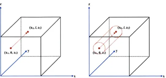
Typical absorption spectra are computed along a line of sight so our first step is to pick a line of sight. Since the gas density varies inside our cosmological box, we are interested in the statistical variation of the spectra over a line of sight so, we want to choose lines at random. First we pick some starting point (x1, y1I, zi).
Then we randomly select a direction in which to travel:
{,
Y,
4}.
Suppose for the sake of example that we choose9.
Then we set yi = 0 and Y2 = 1 where 1 is the length of the box. We set x2, z2 = x1, z1 so that our start and end coordinates are (x1, 0, zi), (x1, 1, z1) as represented pictorially in the left panel of Figure 3-1. Nextwe pick a cylinder or radius r = 0.02 x 1 around this line of sight as depicted in the right panel of Figure 3-1 and keep only simulation data within that cylinder. We then implement periodic boundary conditions because under our assumption of the cosmological principle, if we view the universe on a large enough scale, the distribution of matter is homogeneous and isotropic. Our assumption is justified because we have chosen our box large enough to be representative of the universe at large scales. Once we have chosen the line of sight and the associated cylinder we perform a mesh interpolation of the simulation data over our chosen line of sight to calculate our synthetic spectra.
Z Z
(XI.1 Z2)(X, Z
Z(xi,
0, Z,) :6,Z1
Figure 3-1: In the left panel we show a random line of sight inside a simulation box as described in the text. In the right panel we show this same line of sight along with the cylinder we use for a grid interpolation to obtain data along our line of sight.
3.1.2
Interpolation along line of sight
Once we have chosen our "infinite" cylinder around our line of sight, we can use Python routines to interpolate onto the line. In particular we use the griddata func-tion in the scipy.interpolate module. This method takes in data point coordinates of dimensions (n, D). In our case n varies 2 because it is the number of simulation data
points that fall inside our chosen cylinder and D = 3 because each point is labeled by
a three-dimensional coordinate (x, y, z). We then provide data values of dimension n which are the values of our desired simulated quantites at each of the n data points. Lastly we provide the points at which to interpolate the data which have dimensions (M, D) where M is the number of points along our line of sight that we want data values for and D = 3 as before.
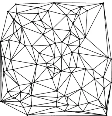
We interpolate onto our line of sight using a linear method. This takes the set of input points and tesselates them onto 2-dimensional simplices 3 where each point is
a vertex on this tesselation, constructed by triangulating the data, and then
per-2As an example in one run n
= 14446 for the first line and n = 27519 for the second line. 3
Simplices are the generalization of a triangle to m dimensions. For example, a 2-simplex is a triangle and a 3-simplex is a tetrahedron.
Figure 3-2: We show an example of the tesselation of varying triangles (2-simplices) on a plane. We use this kind of tesselation to interpolate gas properties along a given line of sight (see text for details) where the vertices are data points obtained from our simulation.
forms a linear barycentric interpolation on each triangle. An example of what such a tesselation might look like in two dimensions is shown in Figure 3-2.
Chapter 4
Computing Ly-a Spectrum
We are now in a position to compute the Ly-a absorption spectrum around our line of sight. We use a readapted version of the method described in Appendix A4 of (Theuns et al. [1998]) for guidance. We first divide our line of sight into 512 bins because that gives us a good enough density of points along our line of sight to have adequate resolution. Each bin is of width A = {-n where 1 is the length of the box.
For a bin i that is at position x(i) we can compute the following
1. Density: the density of neutral hydrogen atoms
2. Density weighted temperature: the temperature distribution taking into ac-count the density of the particles
3. Density weighted velocity: the velocity distribution taking into account the
density of the particles
These are given by the following equations
px(j) = a 3 X(i)Wijp,
(pT)x(j) = a3 X(i)T(i)Wij p
(pv)x(j) = a3ZX(i)(a (i) + (x(i) - x(j)))Wipi. (4.1)
i
We denote X(i) as the abundance of neutral hydrogen, a is the scale factor j, and x are just the positions. The Wij are weight factors obtained from our interpolation
onto the line of sight and pi is the total density in the i-th cell. Then we label the bins according to their velocity from 0 to &L. A bin that has velocity v(k) will have an absorption from the bin at velocity v(j) by an amount e -(kj) where
r(k, j) = o Px(j)aA x exp
[
(4.2)Vx U) V1-T( Vx U)
is the optical depth we introduced in Chapter 2 and
VX
())
(4.3)We have used the following quantities:
1. Vx is the Doppler width of the species with particle mass mx (in our case
neutral hydrogen)
2. A0 = "fA0 is the Ly-a cross section
3. aT = 6.625 x 10⁻²⁵ cm2 is the Thomson cross section
4.
f
= 0.41615 is the oscillator strength of the Ly-a transition5. A0 is the rest wavelength of the transition (for hydrogen A0 = 1215.6 Angstroms.)
As we move forward we refer to e-1 as the transmitted flux. Obviously, anything that is not transmitted is absorbed so when we look at the spectrum of e-', "dips" will correspond to frequencies of light that have not been transmitted and hence absorbed. Therefore the spectrum of transmitted flux is equivalent to an absorption spectrum. In principle if one wanted to compare our results to observations, we could convert the spectrum from absorption at a particular velocity to one that depends on wavelength using
A = A0(1 + z)(1 + # V) ). (4.4)
C
It is important to note that this formulation applies to the SPH method which is dif-ferent from our methods. SPH, as discussed in Chapter 3, uses a Lagrangian method
that discretizes the fluid and talks about the kinematics at these discrete points. Note that this is the point where our method differs from the original formulation presented in (Theuns et al. [1998]), where an SPH code was used and Wij were accordingly the weights of the SPH kernel used to compute the gas density.
4.1
Error Estimation Methods
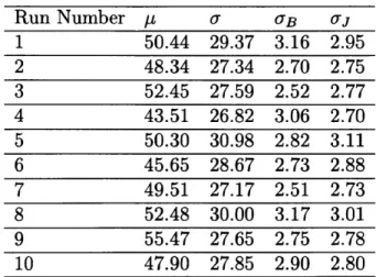
For each choice of redshift and magnetic field we calculated all required quantities for 1000 random lines of sight. Since we assume the universe is isotropic, statistically all these lines of sight can be compared since their direction does not matter. What does matter is that we preserve their length (to be the length of our simulation box) which is taken care of via our method of choosing lines of sight. Then we looked at an average of our statistics over all of these lines and as such we needed to procure an estimate of error bars on our average values of computed statistics. We explored two different methods of estimating the error bars on our simulation data points: the bootstrap method and the jackknife method. We outline both of these methods in the following subsections.
4.1.1
Bootstrap Method
To explain our statistical methods we will work through an example. We begin with a data set {xi} of N = 100 randomly selected numbers in the range (1, 100). The
average of our generated set is p = 50.84 with a standard deviation of o- = 29.23. We then create a new set {xi}1 of 100 points that are randomly sampled with replacement from our original set {xi}. This set will have mean p1. We do this N times to obtain a set of N means {Ii}. The bootstrap error on the mean is then given by
UrB
-N r p b B
4.1.2
Jackknife Method
Consider the same data set {xi} of N = 100 randomly selected numbers in the range (1, 100). We create a new set
{xi}1 = {X2,X3, ... , XN}
by removing the first element in the original set. The mean of this is /.I. We create
N such sets where in set {xi}3 we have removed the jth element of our original set.
The jackknife error on the mean is then given by
N -_1 N
47J = \ -N.12
SN
In our example we obtain oj = 2.94.
When looking at these two methods we should first note that in the formula aj has an added factor of v/N - 1 which could be very large if N was quite large. However,
in the bootstrap method each of our new sets consist of elements from our original set with resampling allowed. Though statistically unlikely, it is possible that one of these resampled sets could contain N copies of the largest element in the original set yielding a really high pi in comparison to p. On the other hand this cannot happen in the jackknife method because the N - 1 elements of the original set have to be
the same which means that ji cannot be that far from p. Hence multiplying o-j by v/N -1 compensates for the large differences in (q, - ,u)2 in the two methods. Notice
that
UB, JJ
-This is a result of the fact that we are finding the standard deviation of the averages that already have a factor of - in them and then multiplying by an additional factor of 1 from the formula for the standard deviation. These error determination meth-ods give us an estimate of how the mean of our sample would fluctuate in response
Run Number 1 o UB Oj 1 50.44 29.37 3.16 2.95 2 48.34 27.34 2.70 2.75 3 52.45 27.59 2.52 2.77 4 43.51 26.82 3.06 2.70 5 50.30 30.98 2.82 3.11 6 45.65 28.67 2.73 2.88 7 49.51 27.17 2.51 2.73 8 52.48 30.00 3.17 3.01 9 55.47 27.65 2.75 2.78 10 47.90 27.85 2.90 2.80
Table 4.1: We perform our statistical test (see text for details) 10 times. Each time we tabulate the mean and standard deviation p, a of our original sample as well as the error on the mean obtained via both estimation procedures aB,
0J-to a change in sampling. In contrast the standard deviation o is a measure of how our sample elements are distributed around the mean.
We concern ourselves now with the difference between these two methods. We per-formed this simple exercise 10 times and obtained the values tabulated in Table 4.1. We notice that aB and oj are always within 0.30 of each other and close to the the-oretical expected value of '. We conclude that for the purpose of our work the two methods are equivalent and we select the bootstrap method for our analysis.
Chapter 5
Results and Discussion
For a given magnetic seed field strength and redshift we choose 1000 lines of sight inside our cosmological box as described in Chapter 3. For each of these lines, we look at the transmitted flux e-' where -r is the quantity defined in Equation 4.2 in Chapter 4 (effectively the absorption spectrum), temperature of the gas, density of neutral hydrogen and the peculiar velocity (velocity with respect to the expansion of the Universe) as a function of distance along each given line of sight. For visualization purposes we consider the line of sight with the following specific endpoints
(0, 0.861 x 1, 0.686 x 1) -+ (1, 0.861 x l, 0.686 x 1)
so it is a line in the X direction. We plot the four aforementioned quantities for this line of sight, B = 10-12 G and z = 2.0 in Figure 5-1. There are a couple of
character-istics to note from the plot of the various spectra. As the density of neutral hydrogen increases the amount of absorption also increases as expected. As such there is a di-rect relationship between the peaks in logl(HI) and the dips in e-. There is also an increase in temperature with density which is expected from the equation of state of this gas discussed in Chapter 2. In Figure 5-2 we look at the variation in the column density of neutral hydrogen over this line of sight. We should compare Figure 5-2 to Figure 5-1. Both figures show a consistent low density region at larger distances and this is consistent with the absorption spectra we see. We can also look at how our
z=2.0 1.0 0.8 0.6 0.4 0.2 0.0 - .0 5 10 15 20 25 L)21 2-12 1 2I,
Figure 5-1: For B = 10-12 G and z = 2.0 we plot the transmitted flux (effectively the
absorption spectrum), the logarithm of the density of neutral hydrogen, the logarithm of temperature of the gas, and the peculiar velocity as a function of distance.
Figure 5-2: We plot the column density
for B = 10-12 G. The horizontal axis is
on the left and right respectively. The (see text) moving in the - direction.
of neutral hydrogen in our cosmological box x in both panels and the vertical axis is y, z
spectra depend on the redshift. In Figure 5-3 we plot the same four quantities for
z = 2.5,3.0. The relationship between redshift z and gas density is a simple result of
the expansion of the Universe. Consider a box with side-length 1 and volume V = 13.
As the universe expands (moving towards smaller z) the length scale changes and the volume of the box gets larger. However, the same amount of gas remains in the box so the density decreases. So, as we increase z, we are increasing the density of our box because we are compressing more into the same volume. Accordingly, we see an increase in the absorption spectrum. Since the density of neutral hydrogen is in-creasing, the temperature also increases proportionally, consistent with the equation of state.
The main point of this work was to look at the variation of the Ly-a spectrum with seed field strength. Keeping the redshift fixed at z = 2.0 we can look at the variation in the spectrum with magnetic seed field strength. We first increase the magnitude to B = 5 x 10 9 G, the spectra is shown in Figure 5-4. Comparing Figures 5-1 and 5-4,
a higher seed field strength appears to give rise to a distribution of neutral hydrogen with less localized gas. There is still less Ly-a absorption at larger distances but there are also some distinct localized areas where there is a lot more absorption than in the low seed field case. We again compare to the column density plots in Figure 5-5. The column density plots show a distribution of hydrogen that is more spread out than for lower field strengths which is in turn consistent with the absorption spectrum we see in Figure 5-4. We can now ask the question as to whether the change in ab-sorption spectrum is a sudden effect or if it gradually changes as we change the field strength. In Figure 5-6 we plot our computed spectra for six different values of the seed field strength: B = {1012, 10-, 10' 0, 10-9,5 x 10⁻⁹, 10-8} G and fixed z = 2.0.
We observe that as we increase the seed field strength we develop more absorp-tion lines closer together. Addiabsorp-tionally larger regions with minimal absorpabsorp-tion, like
d ~ 9 - 13 in Figure 5-6, maintain a consistent level of minimum absorption with
z=2.5 1.0
0.8
0.6
0.4 0.2
Figure 5-3: For B = 10-12 G and z = 2.5, 3.0 we plot the transmitted flux (effectively
the absorption spectrum),the logarithm of the fractional density of neutral hydrogen, the logarithm of temperature of the gas, and the peculiar velocity as a function of distance.
I
z=3 EE7 -3.6 4.4 ...4.2A
.
I 0 -0.6 0.4 28 51015 20 25 - 1 U 0.4 55i~ 10 15302 l-2.f-311
i
-3.2 [1. 0 0.8 i0.6 0.4 0.2 0.0 . 5 10 15 20 25 1.2 -. 6 1"2 0 5101520 25 I'll|& lw (1 01~
Figure 5-4: For B = 5 x 10⁻⁹ G and z = 2.0 we plot the transmitted flux (effec-tively the absorption spectrum), the logarithm of the density of neutral hydrogen, the logarithm of temperature of the gas, and the peculiar velocity as a function of distance.
m ~sr EE
1014 IV 101 10' 6 In
Figure 5-5: We plot the column density of neutral hydrogen in our cosmological box for B = 5 x 10-- G. The horizontal axis is x in both panels and the vertical axis is y, z on the left and right respectively. The dotted white line is our chosen line of
sight (see text) moving in the i direction.
40
1.0 0.8
(
0.6 -, 0.4 G 0 0.0 0 5 10 15 20 25 -15 7.0I W(1 2H1 25 T~I) -;A1Figure 5-6: For varying intensities of B as indicated in the legend and z =2.0 we plot the transmitted flux (effectively the absorption spectrum), the logarithm of the density of neutral hydrogen, the logarithm of temperature of the gas, and the peculiar velocity as a function of distance.
that the transition to more absorption lines is more of an abrupt effect than a gradual one. All of the spectra up to B = 10-9 G appear to be basically the same. The differ-ence is apparent when we increase the seed field above this value. This is consistent with the conclusions made in (Marinacci and Vogelsberger 120151) that the effect of magnetic fields on galaxy population are apparent above a critical seed field strength.
5.1
Flux Probability Density Function
To further understand the effect of the seed field strength on the Ly-a forest we can compute and study the Flux Probability Density Function (Flux PDF). A PDF shows us the probability of attaining a specific transmitted flux (equivalently level of absorption.) We consider e-r for all 1000 LOS individually and make a histogram of these values normalized to 1. We compute error bars via the bootstrap method described in Chapter 4. For z = 0 and B = 10-12, 5 x 10- 9 G this is shown in
Figure 5-7. As per our definition of e-r:
" e -- 0 implies that -r oo so indicates a high level of absorption " e-' 1 implies that -+ 0 so indicates a low level of absorption
In general the trend of the Flux PDF is to increase at lower levels of absorption. This means we have a lower chance of attaining a high absorption. If we compare this to the Ly-a forest spectrum in Figure 5-1 it is consistent with having few absorption peaks. If we look at the curve in Figure 5-7 corresponding to B = 5 x 10⁻⁹ we see
that the general trend is the same, with a slightly higher amplitude. This can be attributed to two factors: there is generally more absorption at a seed field strength above the critical value, as we noticed from Figure 5-6 and the Flux PDF curves down close to e- = 1 for a high magnetic field which allows for a higher probability at
other absorption levels. (The second factor is probably a consquence of normalizing the PDF to 1.) The first factor is more important as it corroborates our statement that there are noticeable effects in the Ly-a spectrum for seed fields above a critical strength.
1 1 *1) -~ 2 _ 0.0 0.2 0.4 0.6 0.8 1.0 (.
Figure 5-7: For z = 2.0 we plot the Flux PDF for B = 10-12 G (with black circles) and B = 5 x 10⁻⁹ G (with blue triangles.)
5.2
Power Spectrum
We can also calculate the power spectrum of the transmitted flux in the Ly-a forest using (Palanque-Delabrouille et al. [2013]) for guidance. The power spectrum gives us the power of the transmitted flux on a specific spatial scale. The larger the power, the more the signal differs from the average of the signal. To compute this we consider e-' for all 1000 LOS. We consider one line 1i with spectrum
fi
= (e-)i and compute the average of e-r over 1i denoted by M. Then we compute the following quantity1
which will have as many elements as points on our LOS. We then take the discrete Fourier transform of this array and let ai be the array of the squared magnitude of the Fourier coefficients. We sum these arrays for all i. The Fourier frequencies are then given by
27r L
where L is the length of our line (1) and k is any integer. This will produce a spectrum symmetric about 0 but we want the power spectrum for positive frequencies so we "fold" 1 the entire spectrum along the v = 0 axis. For z = 2.0 and B =
10-12, 5 x 10- G the power spectrum is shown in Figure 5-8. From Figure 5-8 we
observe that there is less power at higher frequencies. This is most likely because at very small scales there is not enough column density of neutral hydrogen to produce a strong absorption signal. For low intensity seed fields the power spectrum shows a maximum at intermediate scales for a similar reason. It declines at large scales where the density of neutral hydrogen is again probably insufficient enough to give rise to enough absorption. At large seed field strengths the trend is approximately the same but some power has been transferred from the intermediate scales to the larger scale. This is consistent with a more spread out distribution of the gas due to the effects of the magnetic pressure as discussed in Chapter 2.
'By folding we mean associating -vi with vi and adding the two components. Essentially this amounts to keeping the spectrum for v > 0 and doubling its amplitude.
H)'
z=2.0I ** p :
1h' 11-
1()-Frequency
Figure 5-8: For z 2.0 we plot the power spectrum for B 10-12 G (with black
Chapter 6
Conclusions and Summary
Our primary aim in this work was to analyze the effect of varying seed field strength on the morphology of the Ly-a forest. We found that higher magnetic fields affect the spectrum on small scales by producing more absorption lines between already existing absorption lines. This analysis suggests that the effect of seed field strength is an abrupt effect as opposed to a gradual change as the absorption spectrum re-mains basically the same until we introduce a higher-than-critical seed field strength at about 10- G. In order to solidify our claims about the variation in the Ly-a spec-trum we computed the Flux PDF and the Power Specspec-trum of transmitted flux. From the Flux PDF we confirmed that increasing the seed field above the critical strength increases the overall absorption. Our analysis of the power spectrum showed us that independent of the seed field strength the power goes down at very small scales and very large scales because there is not enough column density of neutral hydrogen to produce a strong absorption signal. At intermediate scales the power spectrum has a maximum for the same reason. We also found that at larger seed field strength, again above a critical strength, some power was transferred from intermediate scales to the larger scales. This is consistent with a more spread out distribution of gas due to changes in magnetic pressure.
Additionally, we analyzed the Ly-x spectrum of transmitted flux with varying redshift and found that at higher redshift there was more absorption. This was consistent with
the fact that at higher redshifts there is more neutral hydrogen in the cosmological boxes we studied. This confirms the idea that a higher density of neutral hydrogen results in higher absorption and lower transmitted flux.
There is still room for exploration in this study. We have not extracted all infor-mation from the statistics computed around the Ly-a forest spectrum. An intuitive direction to proceed would be to compare these spectra to observation with the hopes of determining what our simulation analysis could say about the actual values of the seed field strength. Furthermore, understanding more about the seed field can help us to develop a better idea of the events surrounding cosmic inflation.
Appendix A
Cosmology
A.1
ACDM Cosmology
The simulations used in the work were performed under the assumption of a A cold dark matter (ACDM) cosmology. A represents the cosmological constant, associated with a vacuum energy, often referred to as dark energy, in empty space that is most frequently used to explain the accelerating expansion of space against gravity. Dark matter is non-baryonic matter other than that which makes up stars and planets. It is used as an explanation for effects such as the flat rotation curves of spiral galaxies and gravitational lensing. In this model, dark matter is cold which means that its ve-locity is much less than the speed of light. It is also described as being non-baryonic: containing matter other than protons and neutrons. We can explore this cosmology from a general relativity perspective.
As with any cosmological model we start with the action given by
S = d4xv/ Zjg (R - 2A) +
J
d4xL, (gy, I4fM). (A.1)We use notation where R is the Ricci scalar which tells us the curvature of spacetime,
g is the determinant of the metric tensor g,,,, A is the cosmological constant, the
Lagrangian describing a matter field TM.
A.1.1
A Simple Example
To understand what we mean by the matter Lagrangian consider a two particles of mass Mi1, m2 moving in a gravitational field (consider one dimension for simplicity). Then the classical Lagrangian is simply given by
1 *2 1 *2 Gmim2
L = mzi+ -m52 2.(A.2) L 2 1+2. 2 (X1 -X2 2 2)
In this simple model g is our metric tensor g,, since we are only in one dimension and our discretized matter field TM is simply given by the positions and masses of the two particles.
Now that we understand by example what information the matter Lagrangian gives us we can proceed to understand the parameters in this cosmology. We defined the cosmological constant as the energy density of the vacuum. Accordingly it has an equation of state given by the ratio of the pressure PA to the energy density PA which is
PA
WA - -1.
PA
Next we need to define the metric to use for our model. We use the 4-dimensional FLRW (Priedmann-Lemaitre-Robertson-Walker) metric given by
ds2 = -dt 2
+
a2(t)[
r2+ r2dQ211 - Kr2I
where a(t) is the scale factor telling us the expansion of space with time. The pa-rameter K is the cosmic curvature (sometimes denoted using E) taking values 0, +1 corresponding to flat, closed and open universes. As usual dQ2 is the metric of the
spherical solid angle. As in the rest of this work we define the redshift z as a0
z = a
-where ao = 1 is the current scale factor. The Einstein field equations are of the form
1 8irG
RJV - 2 Rgyv+ Agmv = 4 T
and for this model are given by
K2 A K 3 3 a2 and K 2 K H (PM + PM) -2 a
where H = j is the Hubble parameter. Then we define the following quantities:a
1. Fractional density of dark energy: QDE = Pcrit
2. FRactional density of non-relativistic matter: Q.. 3. Fractional density of radiation: Q, = -Jr.
Pcrit
4. Density paramter of the curvature: Qk (aH)2
where pi = . is the critical density and HO is the current Hubble parameter. If
we combine these definitions with the first Einstein equation then
QDE + Qm -+ f2, -+ K = 1
-This is consistent with our knowledge because we would want the total fractional mass density to be 1 in order to have taken care of all space.
A.2
Adiabatic Heating and Cooling
Throughout this work we make references to both adiabatic heating and cooling. An adiabatic process is one that occurs without the transfer of heat or matter between a thermodynamic system and its surroundings; the energy is transferred only as work. Adiabatic heating and cooling refers to the change in temperature of a medium where
there is no transfer but rather all energy is gained or lost via the work done on the medium. In particular, we note that an adiabatic process cannot lead to an excess of free energy.