HAL Id: hal-03012260
https://hal.archives-ouvertes.fr/hal-03012260
Submitted on 10 Dec 2020
HAL is a multi-disciplinary open access
archive for the deposit and dissemination of sci-entific research documents, whether they are pub-lished or not. The documents may come from teaching and research institutions in France or abroad, or from public or private research centers.
L’archive ouverte pluridisciplinaire HAL, est destinée au dépôt et à la diffusion de documents scientifiques de niveau recherche, publiés ou non, émanant des établissements d’enseignement et de recherche français ou étrangers, des laboratoires publics ou privés.
Aseismic deformations perturb the stress state and
trigger induced seismicity during injection experiments
Laure Duboeuf, Louis De Barros, Maria Kakurina, Yves Guglielmi, Frédéric
Cappa, Benoit Valley
To cite this version:
Laure Duboeuf, Louis De Barros, Maria Kakurina, Yves Guglielmi, Frédéric Cappa, et al.. Aseismic deformations perturb the stress state and trigger induced seismicity during injection experiments. Geophysical Journal International, Oxford University Press (OUP), 2021, 224 (2), pp.1464-1475. �10.1093/gji/ggaa515�. �hal-03012260�
Aseismic deformations perturb the stress state and trigger induced seismicity
during injection experiments
Laure Duboeuf (2,1,*), Louis De Barros(2), Maria Kakurina(3), Yves Guglielmi(4), Frederic Cappa(2,5) and
Benoit Valley(3) (1) Now at NORSAR, Gunnar Randers vei 15, Kjeller, Norway
(2) Université Côte d’Azur, CNRS, Observatoire de la Côte d’Azur, IRD, Géoazur, France (3) Centre for Hydrogeology and Geothermics (CHYN), Neuchâtel, Switzerland
(4) Lawrence Berkeley National Laboratory, Berkeley, USA (5) Institut Universitaire de France, Paris, France
* Corresponding author: Laure Duboeuf, [email protected]
Summary
Fluid injections can trigger seismicity even on faults that are not optimally oriented for reactivation, suggesting either sufficiently large fluid pressure or local stress perturbations. Understanding how stress field may be perturbed during fluid injections is crucial in assessing the risk of induced seismicity and the efficiency of deep fluid stimulation projects. Here, we focus on a series of in-situ decametric experiments of fluid-induced seismicity, performed at 280 m depth in an underground gallery, while synchronously monitoring the fluid pressure and the activated fractures movements. During the injections, seismicity occurred on existing natural fractures and bedding planes that are misoriented to slip relative to the background stress state, which was determined from the joint inversion of downhole fluid pressure and mechanical displacements measured at the injection. We then compare this background stress with the one estimated from the inversion of earthquake focal mechanisms. We find significant differences in the orientation of the stress tensor components, thus highlighting local perturbations. After discussing the influence of the gallery, the pore pressure variation and the geology, we show that the significant stress perturbations induced by the aseismic deformation (which represents more than 96 % of the total deformation) trigger the seismic reactivation of fractures with different orientations.
Keywords: Induced seismicity – Geomechanics – Earthquake source observations – Rheology and
I. Introduction
The last decades have shown an large increase of the seismicity induced by fluid injections in the context of industrial activities in oil and gas extraction, geothermal energy production, or CO2
sequestration (Ellsworth, 2013; Elsworth et al., 2016; Healy et al., 1968; Rutqvist, 2012). In fact, between 2008 and 2014, the massive injection of waste-water in the US mid-continent has led to a ~10-fold increase in the seismicity rate for events with Mw>3.5 (Ellsworth et al., 2015). Similarly,
seismicity has been observed during different geothermal activities like in Reykjanes, Iceland (Gudhnason, 2014), Basel, Switzerland (Deichmann & Giardini, 2009), Soult-sous-Forêts, France (Cuenot et al., 2008) or Pohang, South Korea (Grigoli et al., 2018). Moreover, a causal link has been established between fluid injections and the occurrence of aseismic motion (Cornet et al. 1997, Evans
et al. 2005, Guglielmi et al. 2015, De Barros et al. 2016, Duboeuf et al. 2017). Aseismic motions were
observed at large scale in geothermal fields, like for example in Soultz-Sous-Forêts, France (Calò et al., 2011; Cornet et al., 1997), in Geysers, California (Martínez-Garzón et al., 2013) or in Brawley, California (Wei et al., 2015). Several observations and in-situ experiments suggested that fluid injections primarily induced important aseismic motions, and seismicity by stress transfer (Guglielmi et al. 2015, Duboeuf et al. 2017, De Barros et al. 2018, Eyre et al. 2019, De Barros et al. 2019).
The number and magnitude of the induced earthquakes, as well as the seismic/aseismic partitioning (Avouac, 2015; De Barros et al., 2019; Cornet, 2016) depend on the stress state on the faults (Bhattacharya & Viesca, 2019; Galis et al., 2017; Snee & Zoback, 2016; Wynants-Morel et al., 2020) among other parameters. At relatively shallow depth, the stress field may be assessed by borehole measurements (Zang & Stephansson, 2010). For example, Zoback et al. (1985) estimated the in-situ stress orientation using borehole breakout. Combined with observation of drilling-induced tensile fractures, the minimum horizontal stress magnitude can be determined (Hickman & Zoback, 2004), whereas density logs allow computing the vertical stress. Haimson and Cornet (2003) proposed a protocol (HTPF protocol) to determine the stress tensor from leak-off tests conducted on pre-existing natural fractures. Because they require measurements in boreholes, such stress determination methods are technically challenging at large depth and they may be influenced by the stress perturbations in the borehole nearfield. Alternatively, the inversion of earthquake focal mechanisms allows the computation of the principal stress components orientation (e.g. Martínez-Garzón et al., 2016), with a resolution depending on the number and spatial distribution of the seismic events. In fluid injection areas, a discrepancy between the stress states obtained by hydraulic and seismic methods is often observed (Dorbath et al., 2010; Schoenball et al., 2014). In Soultz-sous-Forêts geothermal field, this difference might be explained by the scale of the stimulated volume, as focal mechanism inversion covers a larger stimulated volume than the one considered using borehole measures (Dorbath et al., 2010). Nevertheless, in the same case study, Schoenball et al. (2014) suggest that the stress states computed from focal mechanisms are not representative of the initial stress state existing before the injection. They conclude that borehole determination methods as well as focal mechanisms-based methods may reveal local stress perturbations.
Stress perturbations observed during fluid injections can be induced by a range of physical features and processes including geological heterogeneities, fluid overpressure or aseismic motion. The geological heterogeneities influence – in particular fault zones – was underlined, among others (Shamir & Zoback, 1992; Valley & Evans, 2010), by Faulkner et al. (2006), who showed that the contrast of mechanical properties across a fault zone induces a rotation of the stress field. Studies also show that
fluids can trigger the reactivation of structures mis-oriented to slip in the regional stress state, as for example the main fault on which Ubaye Vallée (France) seismicity occurred (Leclère et al., 2012). Among others studies, Altmann et al. (2014) and Kim & Hosseini (2017) underlined the role of high stimulation pore-pressure in perturbating the stress state in a large stimulated volume. Using a geomechanical modeling approach, Jeanne et al. (2015) related stress perturbations deduced from focal mechanisms inversions (Martínez-Garzón et al., 2013) to changes in fluid injection rates in the Geysers geothermal field (USA). Finally, Schoenball et al. (2014) suggested that an important aseismic motion induced a stress-state rotation during the fluid injections in the GPK2 borehole in Soultz-Sous-Forêts.
Characterizing local stress perturbations is thus a key for proper design of a successful stimulation program and for mitigating the risk of induced seismicity in engineering fluid manipulations in deep reservoirs.In this paper, we compare stress state deduced from earthquakes focal mechanisms with the one deduced from borehole hydraulic tests. These methods, which have been demonstrated individually in several field studies, are combined here to infer the stress within the same stimulation volume and during the same fluid injection tests.
We use data from a controlled induced seismicity experiment at a decameter scale conducted at 280 m depth in a horizontal gallery intersecting a fractured limestone reservoir. The seismicity induced by 11 injection tests was previously analyzed by Duboeuf et al. (2017). Here, we focus on the focal mechanisms in order to determine which geological structures were re-activated during the injections. The earthquake mechanisms are then inverted to reconstruct the stress state. In parallel, the injection borehole displacements continuously monitored during the tests give insights on the stimulated fractures movements which are coupled to stimulation pressures to estimate the static stress tensor using a hydromechanical approach. We compare the hydraulic-based and the focal-mechanism-based stress estimations and we discuss the influence of the tunnel, geology and fluid injection in the observed differences. We conclude that the large aseismic motion measured during these experiments could have triggered significant local stress rotations, resulting in reactivation of misoriented structures.
II. Experimental settings
a. Experimental settings and previous results
The experimental site is located in the Southeast of France sedimentary basin (Figure 1, Jeanne et al., 2013), within the Low Noise Underground Laboratory (LSBB, http://lsbb-new.prod.lamp.cnrs.fr) in which galleries allow a direct access to unaltered cretaceous limestone. We conducted the experiments in a horizontal gallery at 280 m depth where five 20-m long vertical boreholes were drilled in a fractured zone (Figure 1). Eleven fluid injection tests were performed from boreholes B2 and B3 (Figure 1) in different geological structures (fractures, faults, bedding planes) using a hydromechanical probe called SIMFIP (Guglielmi et al. 2013). The probe was composed of two inflatable packers surrounding a 2.4 m-long injection chamber centered on the selected geological structures that we aimed to reactivate during the fluid injection. The probe continuously measured the water pressure, the water temperature and the 3D borehole wall deformation at the injection point, with an accuracy of 0.001 MPa, 0.1 °C, and ~5 μm respectively. A high-resolution network of 24 accelerometers and 9 geophones assured the seismic monitoring. Sensors, located at 4 to 35 m from the injections both on the gallery floor and in the boreholes, scanned a frequency range from 10 Hz to 5 kHz. Thus, induced seismicity, fluid pressure and flowrate, and mechanical deformations were continuously monitored
during the injections (Duboeuf et al., 2017).
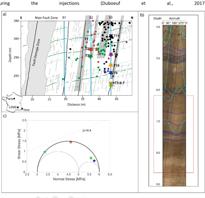
Figure 1 (a) Location of the injection tests and seismicity in a North-South cross-section, adapted from Duboeuf et al. 2017.The colored stars and dots indicate the fluid injection and seismic locations, respectively, colored by test number (Tests 1 in cyan, 2 in red, 3 in green, 5 in grey, 6 in white, 7 in dark grey, 8 in pink, 9 in dark blue, 10 in orange and 11 in black). The 5 vertical boreholes are represented by the blue lines. The inset on the left shows the location of the LSBB facility. (b) is a core sample, showing the BP (dark blue) and F1 (cyan) structures where Test 2 was performed between 6.2 m and 8.6 m depth. The red rectangle shows the position of the injection chamber. (c) Stress-state of the known geological structures (colored stars) in a 3-D Mohr-Coulomb diagram. The grey line represents the rupture for a friction coefficient of 0.4 within the geological stress-state (Guglielmi et al. 2015) and the 3 half-circles the stress tensor.
Here, we present a brief summary of the data processing and interpretation, detailed in Duboeuf and al. (2017). Out of the eleven tests, seven tests (tests 1, 4, 5, 6, 7, 8 and 10) did not induce significant seismicity. We focus on the four tests (tests 2, 3, 9, 11) in which 215 seismic events were identified. 137 events, with moment magnitude lying between -4 and -3.1, were absolutely and relatively located within 1.5 m accuracy. They were found at 1 to 12 m from the injections, suggesting a lack of events at the injection point. Moreover, irreversible deformation was measured for all tests at the injection point. A comparison between the seismic energy and the aseismic deformation shows that more than 96% of the induced deformation occurs aseismically. Both the number and the magnitude of seismic events strongly vary among the tests. Such discrepancy was related to the injected volume when corrected by the amount of aseismic deformations (De Barros et al., 2019). Moreover, the seismic
event distance-to-the-injection variation with injection time does not follow a conventional fluid diffusion law, suggesting the presence of additional effects from other mechanisms related to the observed strain or stress perturbations. From these observations, Duboeuf et al. (2017) proposed that fluid injections drive an aseismic motion that triggers the seismicity.
b. Geology of the stimulated fracture zone
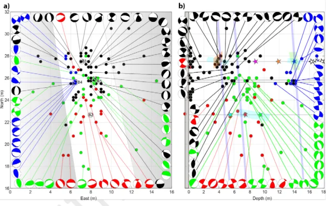
Figure 2 Fault planes and rake distribution, colored by the main geological families: BP (blue), F1 (cyan), F2 (green), and F3 (orange). (a) shows the poles of the main geological structures crossing the injection intervals. (b) shows the poles of the nodal planes of the seismic mechanisms. The colored dots and squares show the interpreted fault and the secondary nodal planes, respectively. Mechanisms without clear geological interpretation are left in grey. (c) is identical to (b) but gathered by fracture families. (d) presents the rake histogram colored by geological structure families. Note that stereographic projections are presented from the lower-hemisphere view, with equal angles.
The experiments took place within the damaged zone of a kilometric normal fault, oriented N030°-85°, that cuts 1-to-5 m thick carbonate layers (Jeanne et al., 2013). This 20 m thick fractured zone contains secondary faults and 1-to-10 m long fractures (Jeanne et al., 2012). The core samples and the boreholes optical logs (Figure 1b) allowed identifying four main families of geological structures intersecting the injection intervals (Figure 2.a) : (1) bedding planes oriented N110° to 135° with a dip angle between 20° and 35°SW (BP), (2) fractures oriented N10° to 30° and dipping 70° E or W (F1), (3) fractures oriented N90° with a dip from 20° to 50°S (F2) and (4) fractures oriented N0° and dipping 45°E (F3). Without considering the structure extensions, these families represent (BP) 26.8 %, (F1) 41.4 %, (F2)
22 %, and (F3) 9.8 % of the identified geological structures (Figure 2.a). All the tests are crossed by F1 structures (Table 1). BP family is not observed in test 3. Finally, Tests 9 and 11 contained few F2 and F3 structures, respectively.
Table 1: Summary of injection depth, identified geological structures, maximum injection fluid pressure and percentage of aseismicity per seismic injection test (Duboeuf et al. 2017).
Test injection
Test Location (depth – borehole)
Geological structures Maximum
injection pressure (MPa)
Aseismic percentage (%)
Test 2 7.5 m depth – B2 BP, and F1 structures. 4.86 97-99.9
Test 3 9.5 m depth – B2 F1 structures 5.3 80-99.9
Test 9 14 m depth – B3 BP, F1 and F2
structures
5.93 98-99.9
Test 11 3.5 m – B3 BP, F1 and F3
structures
5.89 94-99.9
III. Stress state estimation from hydromechanical measurements
The stress state using aseismic fracture displacements and water pressure was computed following the protocols on dislocation analysis during fluid injection and its application to stress inversion developed by Kakurina et al. (2020a, 2020b). The protocol is based on picking the main slip vectors on the test interval fractures, from the continuous SIMFIP borehole displacements recorded during a stimulation test. The main slip vectors correspond to the highest measured slip rates. They may or may not correspond to a seismic event. The rake and plunge of these vectors on the reactivated fracture planes is the starting point for estimating the stress state from a single injection test. The continuous pressure and flowrate records of the SIMFIP probe allow to estimate the normal stress of the activated fracture. It is assumed that the slip vector and the normal opening corresponds to the same activated fracture. The vertical stress exerted on the activated fracture is determined independently by calculating the overburden stress at the depth of the fracture using known density of the carbonate formation (Cochard, 2018). The protocol then searches for the reduced stress tensors, i.e. principal stress orientation and relative magnitude, that are compatible with the slip direction on the reactivated fracture. These reduced stress tensors define the shape of the stress ellipsoids. To determine the magnitude, i.e. sizes of the stress ellipsoids, the protocol searches for the stress ellipsoids that fit the ratio of the normal and vertical stresses on the fracture. The final stress tensors that match all the measurements are resampled by the Monte Carlo method to estimate uncertainties (Walker et al., 1990).
Slip vectors, for the Tests 2, 3, 9 and 11, are oriented 319°/49°, 299°/55°, 105°/69° and 299°/56°, respectively, and are aligned with the structures F1 (Figure 3). Except for Test 3, these slip events occurred before the seismicity. The normal stress from the flowrate-vs-pressure curve was estimated as 1.7, 4.5, 3.2 and 1.7 MPa for Tests 2, 3, 9 and 11, respectively. The vertical stress of 5.7-5.8 MPa was calculated considering the limestone average density of 2.4 g/cm3 and 280 m depth for Tests 2, 3, 9
and 11 (Figure 3). The principal stress orientation and the magnitude between all the tests and with the background stress previously estimated by Guglielmi et al. (2015) give the following full stress tensor : the maximum principal stress 𝜎𝜎1= 6 ± 0.4 MPa is sub-vertical and dips 80°S ± 5; 𝜎𝜎2= 5 ±
0.5 MPa is sub-horizontal and oriented N20° ± 20°; and 𝜎𝜎3 = 3 ± 1 MPa is sub-horizontal and
oriented N110° ± 20° (Guglielmi et al. 2015).
Figure 3 Stress inversion from the hydromechanical data of tests 2, 3, 9 and 11. Upper line shows orientation of the mean principal stress directions (stars) and principal stress uncertainties (small points) determined using the Monte Carlo method. The displacement vector picked in the measurements and projected on the test activated plane. Lower line shows the magnitudes of the principal stresses with the 95 % confidence interval (line) and the mean principal stress magnitude (stars). Blue color corresponds to 𝜎𝜎1, green to 𝜎𝜎2, and red to 𝜎𝜎3.
IV. Stress state estimation from focal mechanisms
a. Method
The focal mechanisms were determined by inverting the first motion polarities of the P-waves. The signal-to-noise ratio allows an unambiguous picking of this polarity on at least 8 stations for 58 events. The inversion was performed using HASH software (Hardebeck & Shearer, 2002, 2003) which integrates errors on the observed polarities, on the event locations (azimuth and take-off angles), and on the velocity model. A set of several possible focal mechanisms is generated using a grid-search on the focal sphere. The preferred focal mechanism is the average of all the possible azimuths, dips and rakes. Uncertainties on the nodal planes are estimated from the root mean square deviation between the preferred focal mechanism and the possible set of solutions.
Even though earthquakes induced by fluid injections may have a non-double-couple component in their focal mechanisms (Julian et al., 1998; Rutledge et al., 2004), we neglected it and assumed a double-couple (DC) mechanism as the non-DC component is usually observed to be only a very small percentage of the rupture (Godano, 2009) and the DC component inversion has shown to be stable even if a small volumetric component is neglected (Šílený & Vavryčuk, 2000).
The earthquake focal mechanisms indicate the fault plane orientation and the slip direction. Assuming the stress field is homogeneous within the considered rock volume and the seismic events slip in the direction of the shear stress on the fault plane, focal mechanisms are used to determine the principal stress field directions by minimizing the difference between the shear stress direction and the seismic event slip directions (Hardebeck & Michael, 2006).
Here, we used a MATLAB package called MSATSI for MATLAB Spatial And Temporal Stress Inversion (Hardebeck & Michael, 2006; Lund & Townend, 2007; Martínez-Garzón, Kwiatek, Sone, et al., 2014). It is based on the Formal Stress Inversion (FSI) method, which is solved by a linearized least-square inversion (Martínez-Garzón, Kwiatek, Ickrath, et al., 2014). A damped inversion is applied on the focal
mechanism dataset, which can be spatially and temporally gathered into smaller subsets. The inversion provides the principal stress orientations and the uncertainties, estimated using a bootstrap resampling method.
b. Focal mechanisms and geological structures
The focal mechanism of 58 events (i.e. 42% of the located events), with magnitude ranging between -3.1 and -4.0, were computed (Figures 2.b.c.d and 4). The mean uncertainty on the nodal plane orientation reaches ~35°. Focal mechanisms show a wide variety of solutions, particularly between the injection tests. They are dominated by reverse motions (Figures 2.d and 4) but they also show normal and strike-slip motions (Figure 4).
Figure 4 Focal mechanisms solution colored by test number (with Tests 2 in red, 3 in green, 9 in dark blue and 11 in black) in (a) a map view, and within the (b) depth-north direction. The figure (a) shows the focal mechanisms with a beach ball representation. Colored dots indicate the event locations. The white and grey areas show the gallery floor and walls. The grey circles show the borehole locations. The figure (b) presents the focal mechanisms into the Depth-North direction. The colored stars indicate the injection test locations. The grey plane shows the gallery floor. Finally, the main identified geological structures that intersect the injection intervals are shown as colored planes (blue for the BP, cyan for the F1, green for F2, and orange for F3).
In order to identify the fault planes from the secondary nodal planes, we compare the focal mechanisms (Figure 2.b) with the geological structures identified in the area (Figure 2.a). Assuming a reduced uncertainty of 20° on the azimuths and 15° on the dip, 31 of the focal mechanisms have one nodal plane that can be linked to one of the main geological families (Figure 2.b). These nodal planes, interpreted as fault planes are related to geological structures as following:
• 7 events (i.e. 22.6 % of the events with identified fault planes) occurred on BP, • 10 events (i.e. 32.2 %) on F1,
• 6 events (i.e. 19.4 %) on F2, • 8 events (i.e. 25.8 %) on F3.
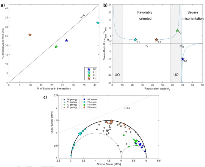
Therefore, focal mechanisms highlight that all known geological structures have been re-activated during the experiment, whatever their orientations toward the stress state. The comparison between the percentage of reactivated fractures with the percentage of identified fractures (Figure 5.a) shows that the reactivation percentage of structures F1, F2 and BP is roughly proportional to their percentage of existence in the medium. Nevertheless, F3, which is less present in the medium shows a larger percentage of reactivation, as discussed later when comparing fracture orientation and stress state. The large heterogeneity in the distribution of the second nodal plane for F1, F2 and F3 families suggests a heterogeneity in the slip motions which is confirmed by the rake distribution (Figure 2.d).
Figure 5 (a) Percentage of reactivated fractures in function of the percentage of fractures into the medium. (b) Stress ratio versus the reactivation angle 𝜃𝜃𝑅𝑅 between 𝜎𝜎𝑚𝑚𝑚𝑚𝑚𝑚 axis and the fault plane for the four main fracture families (stars) that are
reactivated. This figure is adapted from Sibson (1985), with 𝜃𝜃𝑅𝑅* the optimal reactivation angle and the grey area showing the
unfavorably fault orientation. In both panels, BP is dark blue, F1 is cyan, F2 is green and F3 is orange. (c) Stress state of the known geological structures (stars) and seismic events with a determined focal mechanism (dots) in a 3-D Mohr-Coulomb diagram. The grey line represents the rupture for a friction coefficient of 0.4 within the geomechanical stress state (Gugliemi et al. 2015) and the 3 half-circles the stress tensor.
c. Stress state
From the focal mechanisms, we then aim at determining the stress state (Table 2). First, all the focal mechanisms are inverted together assuming a homogeneous stress field (Figure 6.a). The large uncertainties on the principal stress underlines a poorly constrained solution. In order to test the solution stability, random perturbations are applied on the focal mechanisms by adding uncertainties up to 35° for the strike and up to 15° for the dip. Then, the stress state inversion is performed 100
times on catalogs with those random perturbations. The mean solution is almost (± 5°) identical to the first solution, which validates it. Thus, the inversion leads to the following stress orientation:
• the maximum stress 𝜎𝜎1 (blue dots, Figure 6.a) is subvertical and dips 80°E. However, it could
be more horizontal because of the poor azimuth constraint in the East-West direction. • The intermediate stress, 𝜎𝜎2 (green dots), is sub-horizontal and oriented N260° ± 45°.
• The minimum principal stress 𝜎𝜎3 (red dots) is also sub-horizontal and oriented North-South (N175° ± 45°).
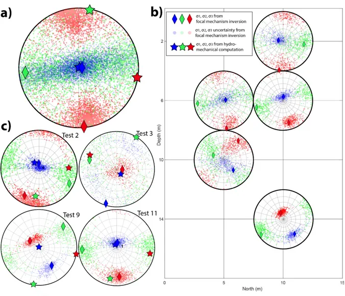
Figure 6 Stress states from the focal mechanism inversion. The stress fields are determined by inverting (a) all focal mechanisms; (b) focal mechanisms gathered by common locations, in a North-Depth cross-section; (c) focal mechanisms gathered by injection tests. The principal stress directions are indicated by the diamond symbol with the specific color: blue for 𝜎𝜎1, green for 𝜎𝜎2, and red for 𝜎𝜎3. The smallest points are the output of the bootstrap resampling used to determine the
uncertainty range, while the diamonds show the best solution. To compare with from the stress states obtained from hydromechanical computation, the principal stress directions are represented by the star symbol.
This stress state therefore shows an inversion of the two horizontal components, compared to the stress state determined by Guglielmi et al. (2015) and by the hydro-mechanical inversion (Figure 3). Such a 90° rotation could indicate a change between 𝜎𝜎2 and 𝜎𝜎3 – i.e. (𝜎𝜎2; 𝜎𝜎3) become(𝜎𝜎3; 𝜎𝜎2)-, which
will be likely if their magnitudes were closed. Here, the large difference between 𝜎𝜎2 and 𝜎𝜎3 magnitudes
amplitude or their orientation. Moreover, this solution is not well-constrained, as highlighted by the very large uncertainties. A possible explanation can be found into a non-homogeneous stress field in the experimental area. We therefore look for spatial variations of the stress field.
The state-of-stress is thus computed at 5 locations along the North-South main trend of events location (Figure 6.b, 1 and 4). Events are gathered on points located at 2, 6, 10, and 14 m depth and on B2 or B3 boreholes, according to their closest location. A variation of the stress tensor orientation with depth is observed:
• at 2 and 6 m depth, 𝜎𝜎1 is sub-vertical while 𝜎𝜎3 and 𝜎𝜎2 are sub-horizontal, approximately oriented N180° ± 45° and N90° ± 30°, respectively. These stress orientations are quite similar to the one obtained from the inversion of all focal mechanisms. This is consistent with the fact that 64 % of the seismicity occurred between the gallery floor and 8 m depth.
• at 10 m depth, 𝜎𝜎1 rotates from subvertical to N135° ± 20°, dipping ~55° ± 7° SE. 𝜎𝜎2 and 𝜎𝜎3 rotate to N290° ± 20°, dipping ~45° ± 7° NW and to N40° ± 30° sub-horizontal, respectively. • at 14 m depth, 𝜎𝜎1 is oriented N140° ± 20° dipping 40° ± 10°SW. 𝜎𝜎2 is sub-horizontal N240° ±
30° and 𝜎𝜎3 dips 85° ± 5°NW.
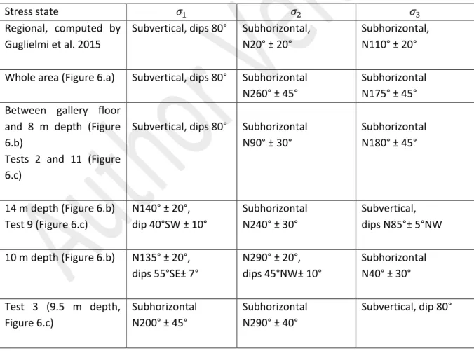
Table 2 Regional stress state and stress states determined using the full set of focal mechanisms, or subsets gathered by depth or test. Dipping angles are considered as subhorizontal when smaller than 10°.
Stress state 𝜎𝜎1 𝜎𝜎2 𝜎𝜎3
Regional, computed by Guglielmi et al. 2015
Subvertical, dips 80° Subhorizontal, N20° ± 20°
Subhorizontal, N110° ± 20° Whole area (Figure 6.a) Subvertical, dips 80° Subhorizontal
N260° ± 45°
Subhorizontal N175° ± 45° Between gallery floor
and 8 m depth (Figure 6.b)
Tests 2 and 11 (Figure 6.c)
Subvertical, dips 80° Subhorizontal N90° ± 30° Subhorizontal N180° ± 45° 14 m depth (Figure 6.b) Test 9 (Figure 6.c) N140° ± 20°, dip 40°SW ± 10° Subhorizontal N240° ± 30° Subvertical, dips N85°± 5°NW 10 m depth (Figure 6.b) N135° ± 20°, dips 55°SE± 7° N290° ± 20°, dips 45°NW± 10° Subhorizontal N40° ± 30° Test 3 (9.5 m depth, Figure 6.c) Subhorizontal N200° ± 45° Subhorizontal N290° ± 40° Subvertical, dip 80°
We then determine the stress state individually at Tests 2, 3, 9 and 11, using a minimum of 6 focal mechanisms to perform each inversion (Figure 6.c). Tests 2 (7.5 m depth), 9 (14 m depth) and 11 (3.5 m depth) display stress states identical to the stress states previously deduced et 6, 14 and 2 m depth (Figure 6.b), respectively. Stress determined for the Test 3 differs from the one determined at 10 m,
but it is badly constrained. We conclude that stress-state computed by event locations or by tests sequence are similar, probably because most of the events gather around their injection area (Figures 1 and 4).
The shallower stress states and Tests 2 and 11 show a 90° rotation of the horizontal stress compared to the stress field inferred from geomechanical data; and the deepest test (9) highlights a 𝜎𝜎1 and 𝜎𝜎3
inversion in addition of the 90° rotation of 𝜎𝜎2. The stress state appears to be heterogeneous within the
experimental site and characterized by changes with depth and/or tests.
V. Comparison between the focal mechanism and the hydromechanical approaches for the estimation of stress
Stress deduced from focal mechanisms inversion differs from stress deduced from displacement-pressure inversion (hereafter referred as geomechanical stress state). We observe a heterogeneity of the seismic-deduced principal stress orientations with depths and/or with the injection tests. In comparison, the principal stress orientations deduced from the hydromechanical approach are very consistent between tests.
a. Reactivation fractures and geomechanical stress field
We first consider the “geomechanical” stress state to calculate the potential for slipping on preexisting geological structures using equation 1 (Sibson, 1985):
𝑅𝑅 = 1+ 𝜇𝜇𝑠𝑠𝑐𝑐𝑐𝑐𝑐𝑐𝑚𝑚𝑐𝑐(𝜃𝜃𝑅𝑅) 1− 𝜇𝜇𝑠𝑠𝑐𝑐𝑚𝑚𝑐𝑐(𝜃𝜃𝑅𝑅) = 𝜎𝜎1′ 𝜎𝜎3′= 𝜎𝜎1−𝑃𝑃𝑓𝑓 𝜎𝜎3−𝑃𝑃𝑓𝑓 , (1)
where 𝑃𝑃𝑓𝑓 is the pore pressure, 𝜇𝜇𝑠𝑠 the friction coefficient (here, 0.4 as determined by Jeanne et al.
(2012) and 𝜃𝜃𝑅𝑅 the angle between the fault plane and 𝜎𝜎1 axis. 𝜃𝜃𝑅𝑅 is computed for all structure families,
and equation (1) solutions are plotted in Figure 5.b, which indicates whether structures are well, unfavorably or extremely mis-oriented to slip in the regional state-of-stress.
Within this stress field, the intermediate stress (𝜎𝜎2) direction belongs to F1 and F3 fault planes (with
angles of 0° and 13°, respectively). Thus, with 𝜃𝜃𝑅𝑅 angles of about 23° and 44° and a ratio R of ~2
(equation 1), F1 and F3 structures are well oriented to slip and a low pore pressure of ~0.7 MPa is required to induce slips. It may explain why they are the most reactivated structures (~32 % and ~26 %, respectively, Figure 5.a). However, although these structures should slip in a normal motion, only half of the observed mechanisms are normal (Figures 2.d and 4).
Figure 5.b indicates that the other geological structures are either unfavorably oriented to slip, like F2, or extremely misoriented, like BP. The angles 𝜃𝜃𝑅𝑅 of about 70° and 65° lead to R ratio of -10 and 8.3 for
BP and F2 respectively. Moreover, 𝜎𝜎3 is within BP and F2 fault planes, as the angle between the fault
planes and 𝜎𝜎3 direction is of 5.7° and 11°, respectively. Rupture should be therefore driven by 𝜎𝜎1 and
𝜎𝜎2. In this case, applying equation 1 leads to a pore pressure of 5.1 MPa and 4.9 MPa, respectively for
BP and F2, in order to reach failure, which is in the range of the maximum injected pressure during Tests 9 and 11 (5.9 MPa). Considering the fluid pressure decays with the distance to the injection point, it is not likely to be above 5.1 MPa where events occurred (1.5 to 12 m to the injection). Finally, BP and F2 structures are also reactivated during Test 2 during which the maximum injection pressure is 4.8 MPa. Consequently, fluid pressure during the injections was not high enough to induce failures on those structures under the assumption of a constant and homogeneous stress state, suggesting that perturbation of stress is required to allow misoriented fractures to slip.
The stress state that applies on all fractures are represented in a shear stress versus normal stress plot, together with the Mohr-Coulomb criterion (Figure 1c and Figure 5c). The normal and shear stress are computed using the Cauchy equation (Jaeger et al., 2009) within the regional stress-state of Guglielmi et al. (2015). It confirms our analysis, showing that while F1 and F3 are relatively well-oriented to slip into the geomechanical stress state, BP and F2 present a strong misorientation for reactivation. Therefore, a fluid pressure of ~5 MPa is required to reach the rupture on these structures.
b. Tunnel and Spatial heterogeneity of the stress field
As the experiments were performed close to a gallery, the tunnel might have influenced local perturbations of the stress state in the so-called Excavation Damage Zone (EDZ, Shen & Barton 1997, Eberhardt 2001, Kaiser et al. 2001). In the EDZ, the vertical stress can be reduced, yielding to a sub-vertical 𝜎𝜎3 and a sub-horizontal 𝜎𝜎1. However, the computed stress state highlights sub-horizontal 𝜎𝜎3
and sub-vertical 𝜎𝜎1. This ~0.5m thin damage zone observed on cores might not be enough to
perturbate stress in these hard carbonate rocks even relatively close to the gallery. Consequently, the cavity presence cannot explain the stress state changes with depth.
In addition, fluid injections are realized in the damaged zone of a normal fault, which presents a high geological heterogeneity. Faulkner et al. (2006) showed that fault structures could drive to a rotation of the stress field, because of the heterogeneities of mechanical properties across the fault zone. However, in our experiments, the injections were all at a similar, relatively large distance (~20 m) from the fault core. So the same stress fault perturbation should influence all the tests. At a smaller scale, similar geological structures are identified at the different injection points. It not likely that they may induce different stress state at a few meters distance. Therefore, the stress heterogeneity may be associated to the different tests, and not to the seismicity locations. As most of the events gather around the injection points, the differences due to the different tests are also visible with depths.
c. Scales effect between the seismic and geomechanical approaches?
The seismic mechanisms correspond to small, decimeter-scale ruptures (De Barros et al., 2019; Duboeuf et al., 2017). The seismic method relates the stress to dislocations on these very localized activated structures, most of them being meters away from the injection source. The geomechanical approach associates the local direct measurement of the slip on a fracture at the injection source with the injection pressure. It appears that whatever the orientation of the activated structure is, there is a consistent estimation of the stress tensor’s orientation and magnitude compared to the seismic approach which highlights a high variability. Main difference is that the geomechanical approach uses slow rupture which correspond to relatively large displacement magnitudes representative of pluri-meter fracture pressurized patches. The seismic approach relies on micrometric displacement on small decimeter scale rupture patches given the low magnitude of the events (Huang et al., 2019). This might explain why there is much more variability of the stresses deduced from seismicity since they may be more sensitive to local heterogeneities such as discontinuities roughness, friction and critical slip distances. Besides our previous work (Guglielmi et al. 2015, Duboeuf et al. 2017, De Barros et al. 2018) showed that aseismic displacements were preceding seismicity, and that events were triggered at and beyond the fluid pressure front. This was related to the shear stress perturbation at the front (Wynants-Morel et al., 2020), which might be the one deduced from the current focal mechanisms approach.
In addition – as neither the fluid pressure nor the presence of the geological heterogeneities directly explain the reactivation of misoriented structures – the large aseismic deformation which continuously varies during the test sequence is an obvious link between stress deduced from seismicity and stress deduced from pressure and displacement. Tests 2, 9 and 11, which contain the misoriented BP and F2 structures, are characterized by more than 96 % of aseismic motion. This aseismic deformation induces stress perturbations at least tens of meters around the pressurized zone and through mixed mode rupture mechanisms (Guglielmi et al. 2015, Wei et al. 2015, De Barros et al. 2018, 2019, Cappa et al. 2019).
At the scale of our experiments, induced seismicity may thus be representative of the stress perturbation induced by aseismic movements on preexisting fractures. Oppositely, the stress state determined from pressure-displacement data might figure a stress state representative of the scale of the stimulated pressurized volume. For the different tests, the amplitude and the direction of the aseismic deformation differ, as the structures in which the fluid is injected differs. It is likely to explain why the reconstructed stress field varies among tests. As the stress field is perturbated in response to the aseismic motion, structures that were misoriented in the regional stress field may, then, be well oriented to slip, with a limited fluid pressure. This has been suggested in Soultz-Sous-Forêts geothermal field, when fluid injections were performed in GPK2 borehole. Schoenball et al. (2014) proposed that the stress state change deduced from induced earthquakes was due to the strong aseismic motion mentioned by Calò et al. (2011). Similarly, in the Brawley geothermal field (California, USA), a strong aseismic motion was recorded on geodetic instruments preceding the seismicity occurrence and specially two large earthquakes with magnitude greater than 5 (Wei et al. 2015). We here propose that fluid injections trigger the aseismic motion which then induces stress perturbation. These stress perturbations allow reactivating fractures with different orientations. Consequently, a significant part of the measured induced seismicity may reveal local stress perturbations more or less distant from the fluid injections. Therefore, for small event magnitudes, the stress state inferred from the focal mechanisms may not be representative of the regional initial stress state, but its heterogeneity may highlight the presence of strong aseismic deformation. At a reservoir scale, heterogeneities in the stress field may also suggest that aseismic deformations trigger seismicity, as suggested by Schoenball et al. 2014 during an injection in Soultz-Sous-Forêts. However, while small events may show heterogeneous mechanisms due to stress perturbations, large earthquakes, with size comparable or larger than the size of the pressurized zone, are likely to be compatible with the regional stress state. Therefore, stress heterogeneities may be visible at very local scales for small magnitude events and they may be masked when averaged at the full reservoir scale. Such statement should be however validated and tested on different reservoir injections by comparing stress-state determined from hydro-mechanical measures in deep boreholes with stress state from seismic mechanisms at different scales.
VI. Conclusion
Here, we studied the seismicity and stress perturbations during a series of fluid-injections performed at 280 m depth in selected geological structures of a carbonate fractured reservoir zone. Comparing the seismic mechanisms with the main geological structures observed in the area, we observed that all fractures families were reactivated, including those that are badly oriented toward the regional stress state. The stress states reconstructed from the inversion of focal mechanisms always differ from the one determined through hydro-mechanical measurements at the locations of the injection. When
using event subsets, we observed that the reconstructed stress states vary with depth and/or tests. The fluid pressure or the geological heterogeneities cannot explain the heterogeneity of the stress field and the reactivation of misoriented structures deduced from the induced earthquakes focal mechanisms. Therefore, we propose that the strong aseismic deformation, precisely measured at the injection, temporarily modifies the stress state, which allows seismic events to be triggered on a large variety of structures, initially misoriented, inside and around the stimulated volume. The perturbed stress fields deduced from seismic mechanisms might then be a qualitative probe of aseismic deformation.
Acknowledgments
We would like to thank the Agence Nationale de la Recherche (ANR) and Total SA company who funded this research through projects HYDROSEIS (ANR
-13-JS06-0004-01) and HPMS-Ca (Albion PI. G.
Massonat
), respectively. We also thank NORSAR (Kjeller Norway) for the use of Mstudio, a NORSAR in-house software package, to generate the Figure 4.b.VII. References
Altmann, J. B., Müller, B. I. R., Müller, T. M., Heidbach, O., Tingay, M. R. P., & Weißhardt, A. (2014). Pore pressure stress coupling in 3D and consequences for reservoir stress states and fault reactivation. Geothermics, 52(Supplement C), 195–205.
https://doi.org/https://doi.org/10.1016/j.geothermics.2014.01.004
Avouac, J. P. (2015). From geodetic imaging of seismic and aseismic fault slip to dynamic modeling of the seismic cycle. Annual Review of Earth and Planetary Sciences, 43, 233–271.
Bhattacharya, P., & Viesca, R. C. (2019). Fluid-induced aseismic fault slip outpaces pore-fluid migration. Science, 364(6439), 464 LP – 468. https://doi.org/10.1126/science.aaw7354 Calò, M., Dorbath, C., Cornet, F. H., & Cuenot, N. (2011). Large-scale aseismic motion identified
through 4-D P-wave tomography. Geophysical Journal International, 186(3), 1295. https://doi.org/10.1111/j.1365-246X.2011.05108.x
Cappa, F., Scuderi, M. M., Collettini, C., Guglielmi, Y., & Avouac, J. P. (2019). Stabilization of fault slip by fluid injection in the laboratory and in situ. Science Advances, 5(3), eaau4065.
https://doi.org/10.1126/sciadv.aau4065
Cochard, J. (2018). Analyse des propriétés réservoirs d’une série carbonatée microporeuse fracturée:
approches multi-échelle sédimentologiques, diagénétiques et mécaniques intégrées.
Aix-Marseille.
Cornet, F. H. (2016). Seismic and aseismic motions generated by fluid injections. Geomechanics for
Energy and the Environment, 5, 42–54.
https://doi.org/http://dx.doi.org/10.1016/j.gete.2015.12.003
Cornet, F. H., Helm, J., Poitrenaud, H., & Etchecopar, A. (1997). Seismic and Aseismic Slips Induced by Large-scale Fluid Injections. In S. Talebi (Ed.), Seismicity Associated with Mines, Reservoirs and
Fluid Injections (pp. 563–583). Basel: Birkhäuser Basel.
https://doi.org/10.1007/978-3-0348-8814-1_12
Cuenot, N., Dorbath, C., & Dorbath, L. (2008). Analysis of the Microseismicity Induced by Fluid Injections at the EGS Site of Soultz-sous-Forêts (Alsace, France): Implications for the
Characterization of the Geothermal Reservoir Properties. Pure and Applied Geophysics, 165(5), 797–828. https://doi.org/10.1007/s00024-008-0335-7
De Barros, L., Daniel, G., Guglielmi, Y., Rivet, D., Caron, H., Payre, X., et al. (2016). Fault structure, stress, or pressure control of the seismicity in shale? Insights from a controlled experiment of fluid-induced fault reactivation. Journal of Geophysical Research: Solid Earth, 121(6), 4506– 4522. https://doi.org/10.1002/2015JB012633
De Barros, L., Guglielmi, Y., Rivet, D., Cappa, F., & Duboeuf, L. (2018). Seismicity and fault aseismic deformation caused by fluid injection in decametric in-situ experiments. Comptes Rendus -
Geoscience, 350(8), 464–475. https://doi.org/10.1016/j.crte.2018.08.002
De Barros, L., Cappa, F., Guglielmi, Y., Duboeuf, L., & Grasso, J.-R. (2019). Energy of injection-induced seismicity predicted from in-situ experiments. Scientific Reports, 9(1), 4999.
Deichmann, N., & Giardini, D. (2009). Earthquakes Induced by the Stimulation of an Enhanced Geothermal System below Basel (Switzerland). Seismological Research Letters, 80(5), 784–798. https://doi.org/10.1785/gssrl.80.5.784
Dorbath, L., Evans, K. F., Cuenot, N., Valley, B., Charléty, J., & Frogneux, M. (2010). The stress field at Soultz-sous-Forêts from focal mechanisms of induced seismic events: Cases of the wells GPK2 and GPK3. Comptes Rendus - Geoscience, 342(7–8), 600–606.
https://doi.org/10.1016/j.crte.2009.12.003
Duboeuf, L., De Barros, L., Cappa, F., Guglielmi, Y., & Seguy, S. (2017). Aseismic motions drive a sparse seismicity during fluid injections into a fractured zone in a carbonate reservoir. Journal of
Geophysical Research: Solid Earth. https://doi.org/10.1002/2017JB014535
Eberhardt, E. (2001). Numerical modelling of three-dimension stress rotation ahead of an advancing tunnel face. International Journal of Rock Mechanics and Mining Sciences, 38(4), 499–518. https://doi.org/https://doi.org/10.1016/S1365-1609(01)00017-X
Ellsworth, W. (2013). Injection-Induced Earthquakes. Science, 341(6142). https://doi.org/10.1126/science.1225942
Ellsworth, W., Llenos, A. L., McGarr, A., Michael, A. J., Rubinstein, J. L., Mueller, C. S., et al. (2015). Increasing seismicity in the U. S. midcontinent: Implications for earthquake hazard. The Leading
Edge, 34(6), 618–626. https://doi.org/10.1190/tle34060618.1
Elsworth, D., Spiers, C. J., & Niemeijer, A. R. (2016). Understanding induced seismicity. Science,
354(6318), 1380–1381. https://doi.org/10.1126/science.aal2584
Evans, K. F., Genter, A., & Sausse, J. (2005). Permeability creation and damage due to massive fluid injections into granite at 3.5 km at Soultz: 1. Borehole observations. Journal of Geophysical
Research: Solid Earth, 110(B4). https://doi.org/10.1029/2004JB003168
Eyre, T. S., Eaton, D., Garagash, D. I., Zecevic, M., Venieri, M., Weir, R., & Lawton, D. C. (2019). The role of aseismic slip in hydraulic fracturing–induced seismicity. Science Advances, 5(8), 1–11. https://doi.org/10.1126/sciadv.aav7172
Faulkner, D. R., Mitchell, T. M., Healy, D., & Heap, M. J. (2006). Slip on’weak’faults by the rotation of regional stress in the fracture damage zone. Nature, 444(7121), 922–926.
Galis, M., Ampuero, J. P., Mai, P. M., & Cappa, F. (2017). Induced seismicity provides insight into why earthquake ruptures stop. Science Advances, 3(12). https://doi.org/10.1126/sciadv.aap7528 Godano, M. (2009). Etude théorique sur le calcul des mécanismes au foyer dans un réservoir et
application à la sismicité de la saline de Vauvert (Gard). Universit{é} de Nice-Sophia Antipolis.
Grigoli, F., Cesca, S., Rinaldi, A. P., Manconi, A., Clinton, J. F., Westaway, R., et al. (2018). The November 2017 Mw 5.5 Pohang earthquake: A possible case of induced seismicity in South Korea. Sciences, 360(June), 1003–1006.
Gudhnason, E. Á. (2014). Analysis of seismic activity on the western part of the Reykjanes Peninsula,
SW Iceland, December 2008-May 2009.
ISRM Suggested Method for Step-Rate Injection Method for Fracture In-Situ Properties (SIMFIP): Using a 3-Components Borehole Deformation Sensor,. Rock Mechanics and Rock
Engineering, 47, 303–311. https://doi.org/10.1007/s00603-013-0517-1
Guglielmi, Y., Elsworth, D., Cappa, F., Henry, P., Gout, C., Dick, P., & Durand, J. (2015). In situ observations on the coupling between hydraulic diffusivity and displacements during fault reactivation in shales. Journal of Geophysical Research: Solid Earth, 120(11), 7729–7748. https://doi.org/10.1002/2015JB012158
Guglielmi, Y., Cappa, F., Avouac, J. P., Henry, P., & Elsworth, D. (2015). Seismicity triggered by fluid injections induced aseismic slip. Science, 348(6240), 1224–1226.
https://doi.org/10.1126/science.aab0476
Haimson, B. C., & Cornet, F. H. (2003). ISRM suggested methods for rock stress estimation—part 3: hydraulic fracturing (HF) and/or hydraulic testing of pre-existing fractures (HTPF). International
Journal of Rock Mechanics and Mining Sciences, 40(7), 1011–1020.
Hardebeck, J. L., & Michael, A. J. (2006). Damped regional-scale stress inversions: Methodology and examples for southern California and the Coalinga aftershock sequence. Journal of Geophysical
Research: Solid Earth, 111(B11). https://doi.org/10.1029/2005JB004144
Hardebeck, J. L., & Shearer, P. M. (2002). A New Method for Determining First-Motion Focal Mechanisms. Bulletin of the Seismological Society of America, 92(6), 2264–2276. https://doi.org/10.1785/0120010200
Hardebeck, J. L., & Shearer, P. M. (2003). Using S/P Amplitude Ratios to Constrain the Focal Mechanisms of Small Earthquakes. Bulletin of the Seismological Society of America, 93(6), 2434–2444. https://doi.org/10.1785/0120020236
Healy, J. H., Rubey, W. W., Griggs, D. T., & Raleigh, C. B. (1968). The Denver EarthquakeS. Science,
161(3848), 1301–1310. https://doi.org/10.1126/science.161.3848.1301
Hickman, S., & Zoback, M. D. (2004). Stress orientations and magnitudes in the SAFOD pilot hole.
Geophysical Research Letters, 31(15), 13–16. https://doi.org/10.1029/2004GL020043
Huang, Y., De Barros, L., & Cappa, F. (2019). Illuminating the Rupturing of Microseismic Sources in an Injection-Induced Earthquake Experiment. Geophysical Research Letters, 46(16), 9563–9572. https://doi.org/10.1029/2019GL083856
Jaeger, J. C., Cook, N. G., & Zimmerman, R. (2009). Fundamentals of rock mechanics. John Wiley & Sons.
Jeanne, P., Guglielmi, Y., Lamarche, J., Cappa, F., & Marié, L. (2012). Architectural characteristics and petrophysical properties evolution of a strike-slip fault zone in a fractured porous carbonate reservoir. Journal of Structural Geology, 44, 93–109.
https://doi.org/http://dx.doi.org/10.1016/j.jsg.2012.08.016
Jeanne, P., Guglielmi, Y., & Cappa, F. (2012). Multiscale seismic signature of a small fault zone in a carbonate reservoir: Relationships between Vp imaging, fault zone architecture and cohesion.
Tectonophysics, 554–557, 185–201.
Jeanne, P., Guglielmi, Y., & Cappa, F. (2013). Dissimilar properties within a carbonate-reservoir’s small fault zone, and their impact on the pressurization and leakage associated with {CO2} injection. Journal of Structural Geology, 47, 25–35.
https://doi.org/http://dx.doi.org/10.1016/j.jsg.2012.10.010
Jeanne, P., Rutqvist, J., Dobson, P. F., Garcia, J., Walters, M., Hartline, C., & Borgia, A. (2015). Geomechanical simulation of the stress tensor rotation caused by injection of cold water in a deep geothermal reservoir. Journal of Geophysical Research: Solid Earth, 120(12), 8422–8438. https://doi.org/10.1002/2015JB012414
Julian, B., Miller, A. D., & Foulger, G. R. (1998). Non-double-couple earthquakes 1. Theory. Reviews of
Geophysics, 36(4), 525–549. https://doi.org/10.1029/98RG00716
Kaiser, P. K., Yazici, S., & Maloney, S. (2001). Mining-induced stress change and consequences of stress path on excavation stability — a case study. International Journal of Rock Mechanics and
Mining Sciences, 38(2), 167–180.
https://doi.org/https://doi.org/10.1016/S1365-1609(00)00038-1
Kakurina, M. (2020). Mechanics of fault reactivation and its application to stress measurement. Centre for Hydrogeology and Geothermics (CHYN), Neuchâtel, Switzerland.
Kakurina, M., Guglielmi, Y., Nussbaum, C., & Valley, B. (2020). In Situ Direct Displacement Information on Fault Reactivation During Fluid Injection. Rock Mechanics and Rock Engineering, 1–16. Kim, S., & Hosseini, S. A. (2017). Study on the ratio of pore-pressure/stress changes during fluid
injection and its implications for {CO2} geologic storage. Journal of Petroleum Science and
Engineering, 149, 138–150. https://doi.org/https://doi.org/10.1016/j.petrol.2016.10.037
Leclère, H., Fabbri, O., Daniel, G., & Cappa, F. (2012). Reactivation of a strike-slip fault by fluid overpressuring in the southwestern French-Italian Alps. Geophysical Journal International,
189(1), 29. https://doi.org/10.1111/j.1365-246X.2011.05345.x
Lund, B., & Townend, J. (2007). Calculating horizontal stress orientations with full or partial
knowledge of the tectonic stress tensor. Geophysical Journal International, 170(3), 1328–1335. https://doi.org/10.1111/j.1365-246X.2007.03468.x
Martínez-Garzón, P., Bohnhoff, M., Kwiatek, G., & Dresen, G. (2013). Stress tensor changes related to fluid injection at The Geysers geothermal field, California. Geophysical Research Letters, 40(11), 2596–2601. https://doi.org/10.1002/grl.50438
Martínez-Garzón, P., Kwiatek, G., Ickrath, M., & Bohnhoff, M. (2014). MSATSI: A MATLAB Package for Stress Inversion Combining Solid Classic Methodology, a New Simplified User-Handling, and a Visualization Tool. Seismological Research Letters, 85(4), 896–904.
https://doi.org/10.1785/0220130189
Martínez-Garzón, P., Kwiatek, G., Sone, H., Bohnhoff, M., Dresen, G., & Hartline, C. (2014).
Spatiotemporal changes, faulting regimes, and source parameters of induced seismicity: A case study from The Geysers geothermal field. Journal of Geophysical Research: Solid Earth, 119(11), 8378–8396. https://doi.org/10.1002/2014JB011385
of focal mechanisms to pore pressure changes. Geophysical Research Letters, 43(16), 8441– 8450. https://doi.org/10.1002/2016GL070145
Rutledge, J. T., Phillips, W. S., & Mayerhofer, M. J. (2004). Faulting Induced by Forced Fluid Injection and Fluid Flow Forced by Faulting: An Interpretation of Hydraulic-Fracture Microseismicity, Carthage Cotton Valley Gas Field, Texas. Bulletin of the Seismological Society of America, 94(5), 1817–1830. https://doi.org/10.1785/012003257
Rutqvist, J. (2012). The geomechanics of CO 2 storage in deep sedimentary formations. Geotechnical
and Geological Engineering, 30(3), 525–551. https://doi.org/10.1007/s10706-011-9491-0
Schoenball, M., Dorbath, L., Gaucher, E., Wellmann, J. F., & Kohl, T. (2014). Change of stress regime during geothermal reservoir stimulation. Geophysical Research Letters, 41(4), 1163–1170. https://doi.org/10.1002/2013GL058514
Shamir, G., & Zoback, M. D. (1992). Stress orientation profile to 3.5 km depth near the San Andreas Fault at Cajon Pass, California. Journal of Geophysical Research, 97(B4), 5059.
https://doi.org/10.1029/91JB02959
Shen, B., & Barton, N. (1997). The disturbed zone around tunnels in jointed rock Masses.
International Journal of Rock Mechanics and Mining Sciences, 34(1), 117–125.
https://doi.org/https://doi.org/10.1016/S1365-1609(97)80037-8
Sibson, R. H. (1985). A note on fault reactivation. Journal of Structural Geology, 7(6), 751–754. https://doi.org/https://doi.org/10.1016/0191-8141(85)90150-6
Šílený, J., & Vavryčuk, V. (2000). Approximate retrieval of the point source in anisotropic media: numerical modelling by indirect parametrization of the source. Geophysical Journal
International, 143(3), 700–708. https://doi.org/10.1046/j.1365-246X.2000.00256.x
Snee, J. E. L., & Zoback, M. D. (2016). State of stress in Texas: Implications for induced seismicity.
Geophysical Research Letters, 43(19), 10,208-210,214. https://doi.org/10.1002/2016GL070974
Valley, B., & Evans, K. F. (2010). Stress Heterogeneity in the Granite of the Soultz EGS Reservoir Inferred from Analysis of Wellbore Failure. World Geothermal Congress 2010.
Walker, J. R., Martin, C. D., & Dzik, E. J. (1990). Confidence intervals for In Situ stress measurements.
International Journal of Rock Mechanics and Mining Sciences & Geomechanics Abstracts, 27(2),
139–141. https://doi.org/10.1016/0148-9062(90)94864-P
Wei, S., Avouac, J. P., Hudnut, K. W., Donnellan, A., Parker, J. W., Graves, R. W., et al. (2015). The 2012 Brawley swarm triggered by injection-induced aseismic slip. Earth and Planetary Science
Letters, 422, 115–125. https://doi.org/http://dx.doi.org/10.1016/j.epsl.2015.03.054
Wynants-Morel, N., Cappa, F., De Barros, L., & Ampuero, J. P. (2020). Stress Perturbation From Aseismic Slip Drives The Seismic Front During Fluid Injection In A Permeable Fault. Journal of
Geophysical Research: Solid Earth, n/a(n/a). https://doi.org/10.1029/2019JB019179
Zang, A., & Stephansson, O. (2010). Stress Field of the Earth’s Crust. Dordrecht: Springer Netherlands. https://doi.org/10.1007/978-1-4020-8444-7
Journal of Geophysical Research: Solid Earth, 90(B7), 5523–5530.