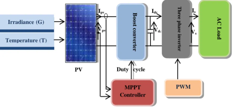
An Optimized Steepest Gradient Based Maximum Power Point Tracking for PV Control Systems.
Texte intégral
Figure


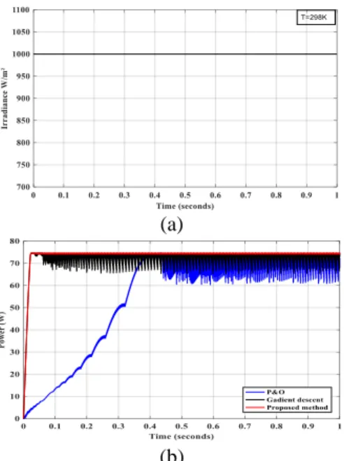

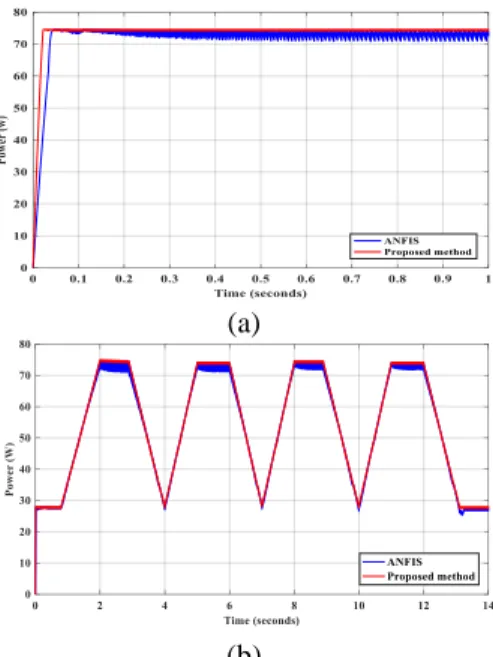
![Figure 18. the PV power supplying according to [31] conditions of G and T.](https://thumb-eu.123doks.com/thumbv2/123doknet/13891256.447419/17.774.281.527.83.251/figure-pv-power-supplying-according-conditions-g-t.webp)
Documents relatifs
In our approach, agents are able to perform collision avoidance during goal directed navigation tasks. We believe that our control scheme can relatively easily be extended to
From equation (1) we notice that the output current of the PV module depends on the photocurrent itself, which itself depends on the solar insolation and the junction temperature of
Abstract - This paper proposes an intelligent control method for the maximum power point tracking (MPPT) of a photovoltaic system under variable temperature and insolation
Maximum Power Point Tracking Control for Photovoltaic System Using Adaptive Neuro-
The purpose of this paper is to study and compare three maximum power point tracking (MPPT) methods in a photovoltaic simulation system using perturb and
In addition, in this method the measurement of the SCC (I SC ) is frequently required which means shorting the module on each occasion. However, by using several loads this issue
Mohamed Aymen SAHNOUN, Hector ROMERO UGALDE, Jean-Claude CARMONA, Julien GOMAND - Maximum power point tracking using P&O control optimized by a neural network approach: a
On graph of time, we can see that, for example, for n = 15 time in ms of conjugate gradient method equals 286 and time in ti of steepst descent method equals 271.. After that, we
