Discrimination levels and perceived duration of intra-
and intermodal short time intervals
Thèse
Leila Azari Pishkenari
Doctorat en psychologie
Philosophiæ doctor (Ph. D.)
Résumé
Cette étude porte sur l’effet de l’intermodalité sur la discrimination de courts intervalles temporels. Chaque intervalle à discriminer est délimité par deux brefs stimuli sensoriels qui sont issus d’une même modalité sensorielle (intervalle intramodal) ou de modalités
sensorielles différentes (intervalle intermodal).
Une série de six expériences, chacune comprenant huit sessions expérimentales, a été réalisée. Une tâche de bissection temporelle a été utilisée dans chacune des expériences de l'étude, sur la base de laquelle on pouvait estimer, pour chaque participant dans chaque condition expérimentale, la sensibilité ou niveau de discrimination (la fraction de Weber) et la durée perçue (l'erreur constante). Selon la loi de Weber, la différence minimale
nécessaire pour distinguer deux stimuli (sensibilité ou seuil différentiel obtenu sur la base de fonctions psychométriques découlant de la tâche de bissection) dépend de leur
magnitude. Le ratio du seuil différentiel à la magnitude devrait être constant. Aussi, plus élevée est la fraction de Weber, moins bon est le niveau de discrimination. Les magnitudes (durées standards) à l’étude étaient de 300 et 900 ms. La durée perçue est évaluée à l’aide de l'erreur constante qui, elle, est mesurée en soustrayant le point d'égalité subjective (PSE, sur chaque fonction psychométrique) de la valeur d’un des intervalles standards (300 ms ou 900 ms). Une valeur inférieure de l’erreur constante signifie que la durée est perçue plus souvent comme "courte".
Il y avait deux séries de trois expériences. Dans la première série, pour une
expérience donnée, la modalité sensorielle du premier marqueur délimitant l’intervalle était la même (condition fixe) et la modalité du second marqueur était variable. Dans la
deuxième série, c'était le deuxième marqueur qui, dans une expérience donnée, restait de la même modalité sensorielle et le premier marqueur était variable. Les marqueurs peuvent être auditifs, visuels ou tactiles. Dans les huit sessions de chaque expérience, il y avait quatre sessions pour chacune des deux conditions de durée standard. Dans chaque expérience, il y avait des conditions de « certitude » et « d’incertitude » relativement à l’origine modale des marqueurs à chaque essai. Les modalités sensorielles utilisées dans chaque étude étaient auditive (A), visuelle (V) et tactile (T).
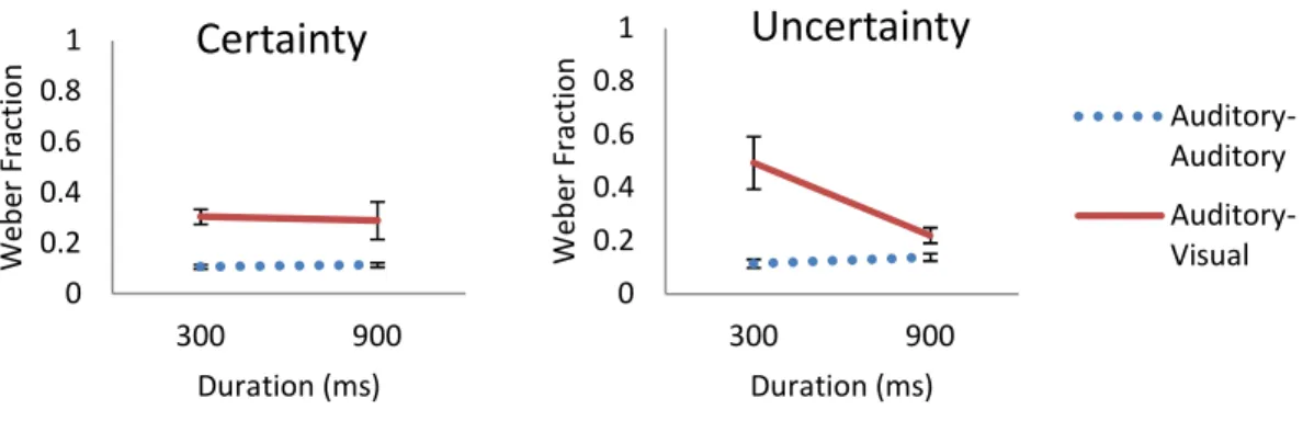
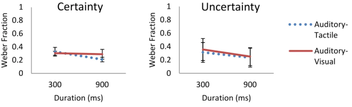
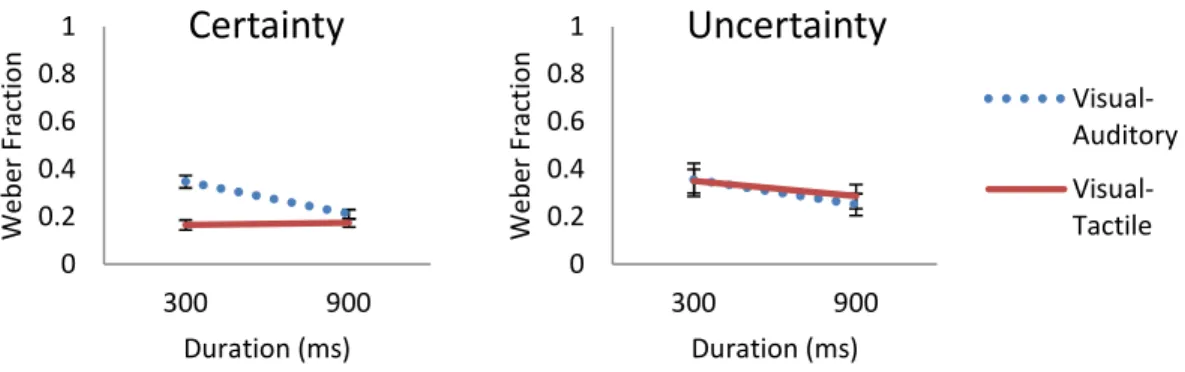
Les résultats montrent que les intervalles intramodaux sont généralement mieux discriminés que les intervalles intermodaux. Aussi, les intervalles de 900 ms sont mieux
discriminés (fraction de Weber plus basse) que ceux de 300 ms dans toutes les conditions de marquage intermodal, mais pas dans les conditions de marquage intramodal où les fractions de Weber demeurent généralement constantes. Le fait que les fractions de Weber soient plus élevées à 300 qu’à 900 ms est compatible avec la forme généralisée de la loi de Weber qui prend en considération le fait que la variance d’origine non temporelle dans le processus de discrimination a plus de poids avec les intervalles courts qu’avec les
intervalles longs. Que les participants connaissent la modalité des marqueurs (certitude) ou non, a peu ou pas d’effet sur le niveau de discrimination.
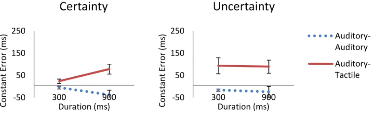
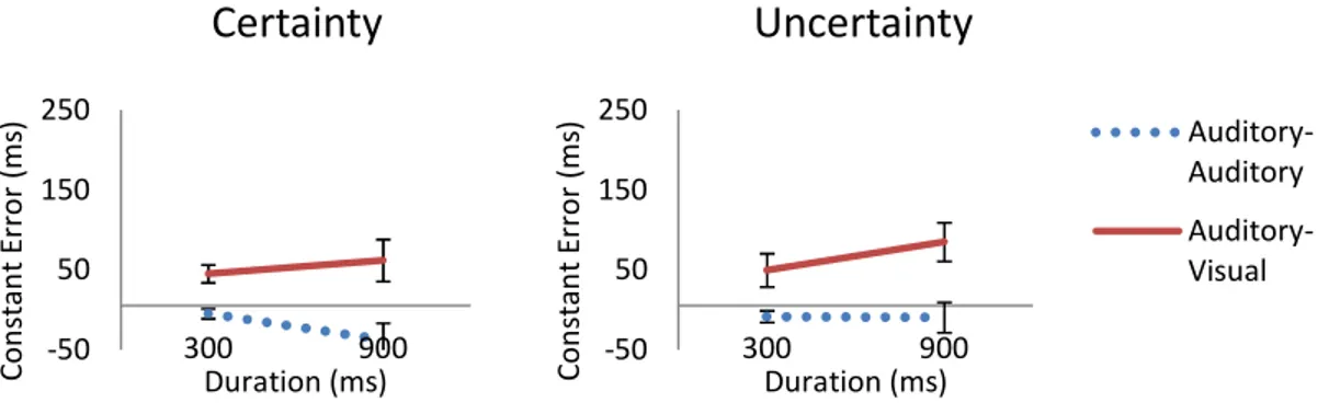
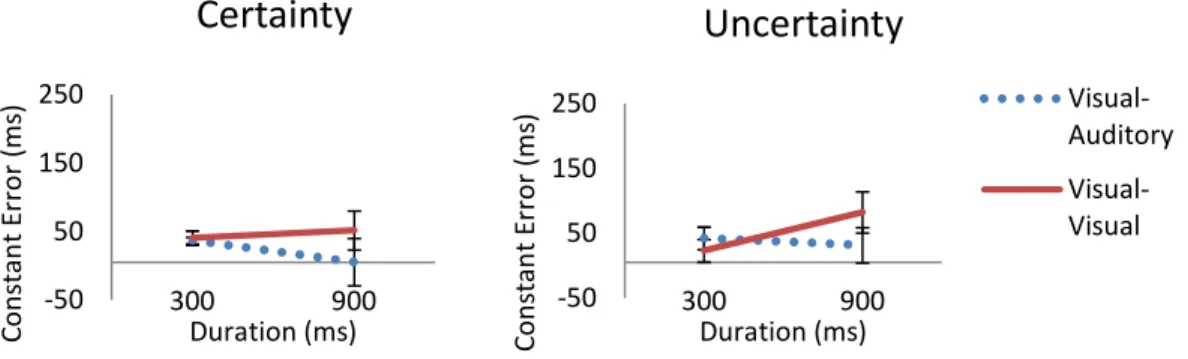
Pour la durée perçue, les résultats révèlent essentiellement ce qui suit. Hormis quelques exceptions, les intervalles intramodaux sont jugés plus courts que les intervalles intermodaux. Dans la comparaison des conditions intermodales, lorsque l’incertitude est placée sur le premier marqueur, il n’y a pas de différences significatives entre les
conditions TA et VA intervalles ou entre les conditions AV et TV, mais les intervalles AT sont perçus comme étant plus longs que les intervalles VT. L’ensemble de ces résultats ne permet pas d’expliquer les différentes durées perçues avec les différents intervalles
intermodaux sur la base de la vitesse nécessaire pour détecter le signal délimitant un intervalle donné.
Pour rendre compte partiellement des différents résultats, on peut s’appuyer sur le modèle de la barrière attentionnelle (Attentional Gate Model - AGM). L’AGM est un modèle d’horloge interne de type pacemaker-accumulateur, le premier module émettant des impulsions dont le cumul détermine la durée perçue (Zakay & Block, 1997). L'AGM contient une barrière et un interrupteur, tous deux sous le contrôle de l’attention. L’efficacité plus grande (plus grande sensibilité) en conditions intramodales qu’en
conditions intermodales proviendrait de l’efficacité du processus de l’interrupteur puisque dans les conditions intramodales, il n’y a pas de déplacement attentionnel d’une modalité à l’autre. Le fait que les intervalles intramodaux, en condition d’incertitude, soient souvent perçus comme étant plus courts que les intervalles intermodaux s’expliquerait par le fait que sans déplacement attentionnel, le deuxième marqueur d’un intervalle intramodal serait détecté plus rapidement que le deuxième marqueur d’un intervalle intermodal. Cependant,
que l’incertitude soit placée sur le premier ou le deuxième marqueur, le niveau de discrimination est peu affecté par celle-ci.
Abstract
This study examines the effect of intermodality on the discrimination of short time
intervals. Every interval in the study is marked by two short sensory stimuli, each of which comes from either the same sensory modality (intramodal interval) or different sensory modalities (intermodal interval).
A series of six experiments, each comprising eight experimental sessions, was carried out. A time bisection task was used in each of the experiments, based on which one could estimate for each participant in each experimental condition, the sensitivity or level of discrimination (the Weber fraction), and the perceived duration (the constant error). According to Weber’s law, the minimum difference necessary to distinguish two stimuli (sensitivity or differential threshold obtained based on psychometric functions arising from the bisection task) depends on their magnitude. The ratio of the threshold difference to magnitude, based on Weber’s law, should remain constant. Also, a higher Weber fraction means a worse level of discrimination. The magnitudes (standard durations) under study were 300 and 900 ms. The perceived duration is evaluated using the constant error, which is measured by subtracting the Point of Subjective Equality (PSE, on each psychometric function) from the value of one of the standard intervals (300 ms or 900 ms). A lower value of the constant error means that the duration is more often perceived as “short”.
There were two sets of three experiments in the study. In the first series, for a given experiment, the sensory modality of the first marker delimiting the interval was the same (fixed condition), and the modality of the second marker was variable. In the second series, it was the second marker which, in a given experiment, remained of the same sensory modality whereas the first marker was variable. Markers could be auditory, visual, or tactile. In the eight sessions of each experiment, there were four sessions for each of the two standard duration conditions. In each experiment, there were also “certainty” and “uncertainty” conditions relative to the modal origin of the markers on each trial. The sensory modalities used in each study were again auditory (A), visual (V), and tactile (T).
The results show that intramodal intervals are generally better discriminated (have a lower Weber fraction) than intermodal intervals. Also, the 900 ms intervals are better
The fact that the Weber fractions are higher at 300 than 900 ms is compatible with the generalized form of Weber’s law, which takes into account the fact that the variance of non-temporal origin in the discrimination process has more weight with short intervals than with long intervals. Whether or not participants know the marker's modality (certainty) has little or no effect on the level of discrimination.
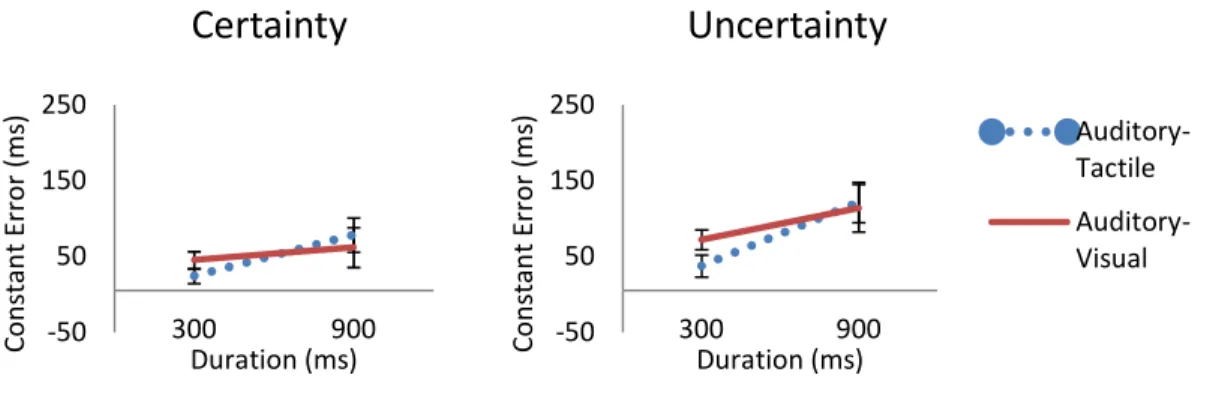
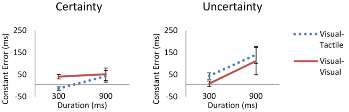
For the perceived duration, the results essentially revealed the following. Except for a few exceptions, intramodal intervals were considered to be shorter than intermodal intervals. In the comparison of the intermodal conditions, when the uncertainty was placed on the first marker, there were no significant differences between the conditions TA and VA intervals or between the conditions AV and TV, but the intervals AT were perceived as being longer than the VT intervals.
To account for the different results in perceived durations, we can rely on the Attentional Gate Model (AGM). The AGM is an internal clock model of the pacemaker-accumulator type, the first module emitting pulses whose accumulation determines the perceived duration (Zakay & Block, 1997). The AGM contains a barrier and a switch, both under attention control. Therefore, according to this model, the greater efficiency (higher sensitivity) in intramodal conditions than in intermodal conditions could come from the efficiency of the switch process. Because in intramodal conditions, there is no attentional displacement from one modality to the other. The fact that intramodal intervals, under conditions of uncertainty, are often perceived as shorter than intermodal intervals could be explained by the fact that without attentional displacement, the second marker of an intramodal interval is detected more quickly than the second intermodal interval marker. However, this explanation encounters certain limits if we consider that, in most cases, whether uncertainty is placed on the first or second marker, the level of discrimination is little affected by it.
Table of Contents
Résumé ... III Abstract ... VI Table of Contents ... VIII List of Figures ... XIII List of Abbreviations ... XVI Acknowledgements ... XVII
Introduction ... 1
Psychophysical Perspective ... 2
The Models ... 4
The interval types ... 8
Attention to time ... 13
Cerebral bases of timing ... 15
CHAPTER 1 ... 18
Objectives and hypotheses... 18
Levels of discrimination ... 20
Perceived duration ... 21
CHAPTER 2 ... 22
General Method ... 22
Apparatus and stimuli ... 23
Procedure ... 23
CHAPTER 3 ... 27
Empirical investigations with ... 27
Marker 1 Fixed and Marker 2 Variable ... 27
Experiment 1: First Marker is Auditory ... 28
Method ... 28
Conditions AA vs. AV ... 29 Conditions AT vs. AV ... 31 Constant Error ... 32 Conditions AA vs. AT ... 32 Conditions AA vs. AV ... 33 Conditions AT vs. AV ... 34 Discussion of Experiment 1 ... 35 Weber fraction ... 35 Constant Error ... 36
Experiment 2: First Marker is Visual ... 37
Method ... 37 Results ... 37 Weber fraction ... 37 Conditions VA vs. VV ... 37 Conditions VT vs. VV ... 38 Constant Error ... 41 Conditions VA vs. VV ... 41 Conditions VT vs. VV ... 42 Conditions VA vs. VT ... 43 Discussion of Experiment 2 ... 44 Weber fraction ... 44 Constant Error ... 45
Experiment 3: First Marker is Tactile... 46
Method ... 46 Results ... 46 Weber fraction ... 46 Conditions TA vs. TT ... 46 Conditions TA vs. TV ... 48 Constant Error ... 50 Conditions TA vs. TT ... 50
Conditions TT vs. TV ... 50
Conditions TA vs. TV ... 51
Discussion of Experiment 3 ... 52
Weber fraction ... 52
Constant Error ... 53
General Discussion of Experiments 1-3 ... 53
CHAPTER 4 ... 56
Empirical investigations with ... 56
Marker 1 Variable and Marker 2 Fixed ... 56
Experiment 4: Second Marker is Auditory ... 57
Method ... 57 Results ... 57 Weber fraction ... 58 Conditions AA vs. TA ... 58 Conditions AA vs. VA ... 59 Conditions TA vs. VA ... 60 Constant Error ... 60 Conditions AA vs. TA ... 60 Conditions AA vs. VA ... 61 Conditions TA vs. VA ... 62 Discussion of Experiment 4 ... 63 Weber fraction ... 63 Constant Error ... 64
Experiment 5: Second Marker is Visual ... 64
Method ... 64
Results ... 65
Weber fraction ... 65
Constant Error ... 68 Conditions AV vs. TV ... 68 Conditions AV vs. VV ... 69 Conditions TV vs. VV ... 70 Discussion of Experiment 5 ... 71 Weber fraction ... 71 Constant Error ... 71
Experiment 6: Second Marker is Tactile ... 72
Method ... 72 Results ... 72 Weber fraction ... 73 Conditions AT vs.TT ... 73 Conditions AT vs. VT ... 74 Conditions TT vs. VT ... 75 Constant Error ... 76 Conditions AT vs. TT ... 76 Conditions AT vs. VT ... 77 Conditions TT vs. VT ... 78 Discussion of Experiment 6 ... 79 Weber fraction ... 79 Constant Error ... 79
General Discussion of Experiments 4-6 ... 80
Weber fraction ... 80
Constant Error ... 81
CHAPTER 5 ... 82
Sensitivity (Weber fraction) ... 84
Perceived duration (Constant Error) ... 87
Applications ... 89
References ... 94
APPENDIX A: ... 101
ANOVA Tables for Experiments 1 to 6 ... 101
APPENDIX B: ... 138
Summary of the goodness-of-fit of the psychometric functions in each portion of each experiment ... 138 Experiment 1: ... 139 Experiment 2: ... 139 Experiment 3: ... 140 Experiment 4: ... 140 Experiment 5: ... 141 Experiment 6: ... 142 APPENDIX C: ... 143
List of Figures
FIGURE 1. ILLUSTRATION OF THE SCALAR EXPECTANCY THEORY OF TIMING. ... 7 FIGURE 2. THE ATTENTIONAL-GATE MODEL OF PROSPECTIVE TIMING ... 8 FIGURE 3. DIFFERENT NEURAL STRUCTURES FOR TIMING. ... 16 FIGURE 4. WEBER FRACTION IN THE A-A AND A-T CONDITIONS UNDER CERTAINTY AND UNCERTAINTY
CONDITIONS... 29 FIGURE 5. WEBER FRACTION IN THE A-A AND A-V CONDITIONS UNDER CERTAINTY AND UNCERTAINTY
CONDITIONS... 31 FIGURE 6. WEBER FRACTION IN THE AT AND AV CONDITIONS UNDER CERTAINTY AND UNCERTAINTY
CONDITIONS... 32 FIGURE 7. CONSTANT ERROR IN THE AA AND AT CONDITIONS UNDER CERTAINTY AND UNCERTAINTY
CONDITIONS... 33 FIGURE 8. CONSTANT ERROR IN THE AA AND AV CONDITIONS UNDER CERTAINTY AND UNCERTAINTY
CONDITIONS... 34 FIGURE 9. CONSTANT ERROR IN THE AT AND AV CONDITIONS UNDER CERTAINTY AND UNCERTAIN
CONDITION. ... 35 FIGURE 10. WEBER FRACTION IN THE V-A AND V-V CONDITIONS UNDER CERTAINTY AND UNCERTAINTY
CONDITIONS... 38 FIGURE 11. WEBER FRACTION IN THE V-T AND V-V CONDITIONS UNDER CERTAINTY AND UNCERTAINTY
CONDITIONS... 39 FIGURE 12. CONSTANT ERROR IN THE VA AND VT CONDITIONS UNDER CERTAINTY AND UNCERTAINTY
CONDITIONS... 41 FIGURE 13. CONSTANT ERROR IN THE VA AND VV CONDITIONS UNDER CERTAINTY AND UNCERTAINTY
CONDITIONS... 42 FIGURE 14. CONSTANT ERROR IN THE VT AND VV CONDITIONS UNDER CERTAINTY AND UNCERTAINTY
CONDITIONS... 43 FIGURE 15. CONSTANT ERROR IN THE VA AND VT CONDITIONS UNDER CERTAINTY AND UNCERTAINTY
CONDITIONS... 44 FIGURE 16. WEBER FRACTION IN THE TA AND TT CONDITIONS UNDER CERTAINTY AND UNCERTAINTY
CONDITIONS... 47 FIGURE 17. WEBER FRACTION IN THE T-T AND T-V CONDITIONS UNDER CERTAINTY AND UNCERTAINTY
CONDITIONS... 48 FIGURE 18. WEBER FRACTION IN THE TA AND TV CONDITIONS UNDER CERTAINTY AND UNCERTAINTY
FIGURE 19. CONSTANT ERROR IN THE TA AND TT CONDITIONS UNDER CERTAINTY AND UNCERTAINTY CONDITIONS... 50 FIGURE 20. CONSTANT ERROR IN THE TT AND TV CONDITIONS UNDER CERTAINTY AND UNCERTAINTY
CONDITIONS... 51 FIGURE 21. CONSTANT ERROR IN THE TA AND TV CONDITIONS UNDER CERTAINTY AND UNCERTAINTY
CONDITIONS. ... 52 FIGURE 22. WEBER FRACTION IN THE AA AND TA CONDITIONS UNDER CERTAINTY AND UNCERTAINTY
CONDITIONS... 58 FIGURE 23. WEBER FRACTION IN THE AA AND VA CONDITIONS UNDER CERTAINTY AND UNCERTAINTY
CONDITIONS... 59 FIGURE 24. WEBER FRACTION IN THE TA AND VA CONDITIONS UNDER CERTAINTY AND UNCERTAINTY
CONDITIONS... 60 FIGURE 25. CONSTANT ERROR IN THE AA AND TA CONDITIONS UNDER CERTAINTY AND UNCERTAINTY
CONDITIONS... 61 FIGURE 26. CONSTANT ERROR IN THE AA AND VA CONDITIONS UNDER CERTAINTY AND UNCERTAINTY
CONDITIONS... 62 FIGURE 27. CONSTANT ERROR IN THE TA AND VA CONDITIONS UNDER CERTAINTY AND UNCERTAINTY
CONDITIONS... 63 FIGURE 28. WEBER FRACTION IN THE AV AND TV CONDITIONS UNDER CERTAINTY AND UNCERTAINTY
CONDITIONS... 66 FIGURE 29. WEBER FRACTION IN THE AV AND VV CONDITIONS UNDER CERTAINTY AND UNCERTAINTY
CONDITIONS... 67 FIGURE 30. WEBER FRACTION IN THE TV AND VV CONDITIONS UNDER CERTAINTY AND UNCERTAINTY
CONDITIONS... 68 FIGURE 31. CONSTANT ERROR IN THE AV AND TV CONDITIONS UNDER CERTAINTY AND UNCERTAINTY
CONDITIONS... 69 FIGURE 32. CONSTANT ERROR IN THE AV AND VV CONDITIONS UNDER CERTAINTY AND UNCERTAINTY
CONDITIONS... 70 FIGURE 33. CONSTANT ERROR IN THE TV AND VV CONDITIONS UNDER CERTAINTY AND UNCERTAINTY
CONDITIONS... 71 FIGURE 34. WEBER FRACTION IN THE AT AND TT CONDITIONS UNDER CERTAINTY AND UNCERTAINTY
CONDITIONS... 74 FIGURE 35. WEBER FRACTION IN THE AT AND VT CONDITIONS UNDER CERTAINTY AND UNCERTAINTY
FIGURE 36. WEBER FRACTION IN THE TT AND VT CONDITIONS UNDER CERTAINTY AND UNCERTAINTY CONDITIONS... 76 FIGURE 37. CONSTANT ERROR IN THE AT AND TT CONDITIONS UNDER CERTAINTY AND UNCERTAINTY
CONDITIONS... 77 FIGURE 38. CONSTANT ERROR IN THE AT AND VT CONDITIONS UNDER CERTAINTY AND UNCERTAINTY
CONDITIONS... 78 FIGURE 39. CONSTANT ERROR IN THE TT AND VT CONDITIONS UNDER CERTAINTY AND UNCERTAINTY
CONDITIONS... 79 FIGURE 40. THE ATTENTIONAL-GATE MODEL OF PROSPECTIVE TIMING ... 87
List of Abbreviations
AA Auditory-Auditory AT Auditory-Tactile AV Auditory-Visual VV Visual-Visual VA Visual-Auditory VT Visual-Tactile TT Tactile-Tactile TA Tactile-Auditory TV Tactile-VisualAcknowledgements
Accomplishing this thesis would not have been possible without the support and collaboration of many people whom I would like to sincerely thank.
First, I would like to express my sincere gratitude to my advisor Prof. Simon Grondin. I thank him today for sharing with me his passion and vast knowledge in the world of research. He gave me the opportunity to discover and participate in this extended world. He also showed me that no matter what language you speak with, no matter which side of the world you live in, and how far from your real home you are, there are always kind people that can make you feel at home--people who remind you of the beauty of the human soul. Thank you Prof. Grondin for not only your advice, your encouragement, your immense availability, but also your unconditional support and kindness. These last years have not always been easy for me, but I always knew that you were there to help me and that I could invariably count on your support. I could not have imagined having a better advisor and mentor.
The substantial support of the members of my advisory committee, Prof. Bastien and Prof. Rousseau, had a formative role in the completion of this dissertation. They
accompanied me throughout my Ph.D. and shared their respective expertise with me. I want to thank them for their interest in my work. Their comments and questions allowed me to further my thoughts and motivated me to continue and helped me to widen my research from various perspectives. I also would like to extend my sincere appreciation to my other committee members: Prof. Yves Lacouture and Prof. Massimo Grassi who generously offered their time, support and guidance in reviewing my dissertation. Their insightful suggestions helped me to improve various aspects of my study.
These years of studies would not have been the same without the support of my very kind lab mates. I have been fortunate to have them beside me in all the complicated and sometimes confusing situations. My friends Giovanna, Pauline, Félix, Guillaume, Joanie, Vincent, Emi, Émie, Daniel. I am very grateful for your 'being there'.
My sincerest thanks are extended to my friends on both sides of the ocean; Alireza, Nafiseh, Farid, Sahar, Parnian, Parnaz, Farid, our petit Nikan whose birth brought a lot of love, joy, and smile to our life in this side of the world. My dear Ziba who, in spite of all
the mountains and seas between us, has always been in my mind and heart, and her presence, no matter what situation I was in, always shed beautiful colors on my life. And finally, Maryam that her friendship and kindness was worth way more than I could ever express on paper. I cannot thank you enough Maryam, you have been here for me literally through sickness and health! And there is no way for me to present you the depth of my gratitude. I only can say that I am sincerely grateful for having you in my life.
An exceptional word of gratitude should go to my family, to my father Abolhassan and my brother Farshid, who supported me wholeheartedly. They have been with me all the time that I was far, far away from home.
I know you went through a lot of difficulties the years I have been in such a long distance from you, I know that the world has not been so kind all these years, that I could not be there for you, but I want you to know that you have been in my heart every single moment of my long long voyage.
Last but not least comes Amin. I know that no step of this long journey could have happened without him--my best friend. Thank you, my dearest Amin, for your precious supports during all these years. Tons of things happened during recent years that could have led – and indeed sometimes did- to a deep state of discouragement in me. I am most
grateful that you have been there for me through it all, and always gave me the strength and motivation along this long sometimes bumpy path. I could not have imagined crossing all the bridges I passed in this period of my life without your unmitigated presence. Thank you for your endless patience, encouragement, and friendship.
Introduction
Time is one of the mysterious concepts in the world. Poets, philosophers, and scientists have all had their struggle with this puzzling notion. Its ubiquity in our conscious life makes us wonder about it even more. Most activities in our daily life such as waiting for a green light, crossing a street, meeting a friend, and participating in sports are
completely dependent on our temporal perception. Time is also crucial to our perception of events, rhythm, and music, and despite people’s arguments for the unreality of time
(McTaggart’s is the most famous among them), we still need to assume its subjective existence in order to account for such phenomena in our everyday life. In fact, subjective experience of time enables us to coordinate our actions and thoughts as well as anticipating forthcoming events (Bechara et al., 1996; Kotz et al., 2009; Nussbaum et al., 2006). This entanglement of the subjective time with our actions, thought and behavior is the main reason explaining why we focus on psychological time rather than on time per se. William James was among the pioneers in the studies of psychological time because he was among the few who changed the course of the studies from mere philosophical speculations to empirical research. In other words, he was the one who shifted the attention from time to psychological time (Roeckelein, 2008).
Empirical studies on psychological time have been conducted in various fields of psychology and neuroscience (Grondin, 2017, 2018). The objectives of each field differ; therefore, the questions that the researchers try to answer vary from one field of study to another. Different questions ask for different methods, yet, there are certain methods that have been firmly established in the psychology of time and some of them are presented in the section about methods. Along with different methods, some of the key concepts, like different intervals, are also introduced, and their applications are explained. Since the study at hand is from a psychophysical perspective, the focus is mostly on the studies of this field. The appropriate models for explaining time experiences are then introduced and, given the nature of this study, the models that are based on central-clock mechanism receive more attention. Furthermore, the issue of attentiveness to time will be discussed
after introducing the models. The section on the purpose of the current study and the relevant information about the experiments will conclude the introduction.
Psychophysical Perspective
There are three main avenues of research in the psychology of time: 1)
psychophysical perspective, 2) animal-behavior perspective, and 3) cognitive perspective. There are, indeed, number of studies which combine these perspectives in order to address their specific questions. The prevalent theme of the time perception studies is to evaluate the subject’s response: 1) when s/he is asked to estimate/scale the duration of the stimulus, and 2) when s/he is asked to discriminate the stimulus lengthwise (discrimination tasks are mainly conducted by using very short intervals which are susceptible to be confused in perception) (Allan, 1979).
The distinctive feature of the studies in psychophysics is the efforts that are made in order to come up with a relation between stimuli, on the one hand, and the subjects’
sensation, on the other. In the case of psychological time, this relation is between estimated/psychological time (sensation) and physical/chronometric time (stimulus). There are various methods to find the relation between the estimated time and the physical time of the stimuli (Stevens, 1975). For instance, in one method, subjects are first presented with a modulus (a standard interval of certain duration) and then are asked to ascribe certain magnitude to the stimuli which follow the modulus. The experimenter ascribes a magnitude to the modulus, hence the subjects’ perception of the duration of stimuli are based on his judgment of the duration of the stimulus. The result of finding the relation between estimated time and chronometric time are normally presented on the two axes of a graph wherein y-axis is the estimated time and x-axis the duration of the stimuli (Grondin, 2008).
Traditionally, there are four main methods in the field of time perception for
assessing the capability of subjects to keep track of time: 1) Verbal estimation—they might be asked to verbally express their perception in time units (seconds, or minutes), 2)
reproduction—in which they are asked to reproduce the interval’s duration by some apparatus, 3) production—in which they are asked to produce a specific target interval
duration of different stimuli. Such a method makes it possible to estimate difference threshold (sometimes called Just Noticeable Difference, JND), which is the minimum time difference required for a subject for discriminating two time intervals (Grondin, 2001, 2010a).
In psychophysics, Weber's law is used in order to describe human perception as a function of stimuli. According to Weber law, the difference threshold is proportional to the magnitude of the stimuli. As we mentioned before, the stimuli in time perception tasks are time intervals, which can be marked with stimuli delivered from different modalities. In discrimination tasks, Weber fraction is the standard measure of acuity of discrimination. Weber fraction may be calculated as the standard deviation of the estimates of the stimulus divided by the magnitude of the stimulus (Luce & Galanter, 1963). Weber function and determining Weber coefficients, as we shall see, are one of the main concerns of this study. One way to determine JND is to use two-alternative forced choice procedure (2AFC), which is to show two consecutive intervals to the subject and ask him/her to compare the second interval’s duration with the first. 2AFC is conducted in two ways: reminder, and roving. In a reminder method, the standard interval is always presented first, while in the roving method, the places of standard and comparison intervals interchange (Macmillan & Creelman, 1991). Reminder method is preferred in discrimination tasks and the subjects’ responses are more accurate in this method. Further to these two methods, in 2AFC, there are two main categories of methods for measuring the difference threshold: 1) constant stimuli, and 2) adaptive stimuli (Grondin, 2008). In the constant method, several
comparison intervals are being presented and the subject is to judge whether the intervals are shorter or longer than the standard interval. The comparison intervals are determined in advance and are not to be changed during the task.
With adaptive stimuli, on the other hand, the comparison intervals are not
predetermined. They are being adjusted according to the subject’s responses. For example, if the subjects make accurate estimations of whether the comparison intervals are longer or shorter than the standard, they are subsequently presented with the comparison intervals which are closer to the standard. One advantage that constant method has over adaptive method is that, since the comparison intervals are predetermined, it would be easier to draw a psychometric function from the subjects’ responses (Grondin, 2008).
Another comparison method is called bisection, and has been prevalent in recent time studies. Bisection is a subcategory of the single-stimulus method, wherein instead of comparing two consecutive intervals, the subjects are asked to put an already presented interval under the categories of either short or long. In bisection method, the shortest and longest intervals (anchors, or standards) or a series of intervals are first presented several times and are then followed by intervals that have to be categorized as being closer to one of the two anchored standards (Grondin, 2010a). The bisection method is normally applied in animal studies, but since animals appear to share basic similarities in their ability to discriminate the durations of events in the seconds-to-minutes range, this method, or the result of animal studies, can also be fruitful in studies on humans (Penney, Gibbon, & Meck, 2008).
The Models
Models in the psychology of time have to account for our experiences of temporality in real-world events, such as speech, music, or movement. Furthermore, in the experimental setting, they are to explain different phenomena that we observe in scaling, and in
discrimination tasks. The tasks, as we have seen, are designed by using various modalities, and different arrangement of markers. Thus, each model has to account for the phenomena that come with inter- or intra- modalities. In addition to this, there are, on the part of subjects, errors in time perception which models need to explain.
There are generally two kinds of models of timing behavior: one assumes the existence of a central clock and the other claims that this assumption is not needed (Zeiler, 1998). Let us start with the latter: The no-central-clock models, sometimes called cognitive models, are prevalent in the studies whose main interest is in human motor timing, animal learning, or human cognition. These models argue that some other mechanisms, for example, a general learning model (Hopson, 2003), is sufficient for explaining our timing behavior. A recent class of no-central-clock models is called intrinsic models. One salient example of such models is referred to as state-dependent network (Buonomano, 2005). In this model, timing is not based on a central clock, but on temporal changes in the state of
duration of a stimulus depend on the operation of dedicated neural mechanisms specialized for representing the temporal relationships between events. Alternatively, the representation of duration could be ubiquitous, arising from the intrinsic dynamics of non-dedicated neural mechanisms. In such models, duration might be encoded directly through the amount of activation of sensory processes or as spatial patterns of activity in a network of neurons (Ivry & Schlerf, 2008).
Some modality-specific models have been developed in the field of visual
perception. In such models, when a flickering stimulus is presented in a specific region of visual space and leads to local adaptation, there is a reduction of the perceived duration of stimuli if they are presented in the same specific region, but not if they are presented in other regions of visual space (Johnston, Arnold, & Nishida, 2006). This links the perception of time to local stimuli and not necessarily to a central clock. Some of the no-central-clock models implement attentional and memory mechanisms in order to account for time behavior. These models normally explain the time phenomena that occur in long intervals (Ornstein, 1969).
Most pieces of the literature on time studies, particularly the ones with a
psychophysical perspective, assume a central mechanism for time processing. This central mechanism can be modeled in three ways: 1) the oscillator process, and 2) the pacemaker-counter process, 3) central mechanisms that are neither oscillators nor pacemaker-pacemaker-counters (Grondin, 2010a).
In the oscillator process, the task of the timing system is to synchronize attention with the pulses that come from the stimuli. In doing so, an oscillatory process is assumed which is made of two components: a nonlinear oscillator, and attentional energy pulse rhythm. The theory behind it is called Dynamic Attending Theory (DAT), which is proposed and aimed at explaining how listeners respond to systematic change in everyday events while retaining the general rhythmic structure of the stimuli (Large & Jones, 1999). The gist of the theory is based on the fact that: first, there are temporal regularities in the environments (in music, in speech, or etc.); second, these regularities mark the coherent beginnings and ends for several succeeding time spans. This temporal regularity makes forthcoming events predictable and sets (within and observer) an attending attitude (Jones & Boltz, 1989). DAT describes attending as the behavior of internal oscillations, called
attending rhythms, that are capable of entraining to the flow of external events and targeting attentional energy to excepted points in time (Large & Jones, 1999). In this model, the internal oscillator changes gradually and adapts to allow the attentional rhythm to get closer to the stimuli onset which eventually leads to synchronization of attentional pulses and stimuli onset. The oscillator in nonlinear and can adapt according to the temporal structure of environmental stimuli (Large, 2008). The oscillator, in this model, continues to adapt until the attentional peaks are well aligned with the expected stimulus onsets. As one might have noticed, DAT and its entrainment strategy are mostly well suited to the phenomena that have regularities built into them. It is unknown how the mechanism would work with the stimuli, such as two marker intervals, which do not necessarily have embedded regularities (Grondin, 2010a).
Another central clock model is the so-called pacemaker-counter device. According to this model, the internal clock is comprised of a pacemaker, which emits pulses, and a counter, which accumulates those pulses. In this model, the pacemaker generates pulses that are accumulated in the counter (Allan, 1979). Any judgment about time duration is based on the number of pulses that are accumulated in the counter. It is obvious that in this model the properties of these pulses, i.e. their rate and fluctuation, is a crucial factor in representing the duration estimation (Grondin, 2010a).
The pacemaker-counter model is not only straightforward but also surprisingly powerful in explaining timing behavior. The elaborated theory based on this model, which is also the most cited one, is called Scalar Expectancy Theory (SET) or Scalar-Timing Model (STM). The theory emphasizes on three levels of information processing: 1) perceptual (clock), 2) memory and 3) decision making. The general idea of SET in comparing two intervals is that clock, which is at the level of perception, causes the accumulation (Figure 1).
Figure 1. Illustration of the Scalar Expectancy Theory of timing (from Allman et al., 2014).
There are several stages in SET at which timing errors might emerge. The reliability of the pacemaker is one of the sources of errors. Different models assume different rates of pulse generation for the pacemaker based on their assumption of whether the pulse
generation follows a linear or a stochastic pattern. The counting system can be a source of errors as well (Killeen & Taylor, 2000). Switch and marking errors is another source of timing errors. The switch is the part of the clock process that is directly associated with the mechanisms of attention. When the switch is closed, the pulses that are emitted by the pacemaker are accumulated in the counter. Indeed, it is the amount of attention paid to time that determines the accumulation of pulses in the counter (Grondin, 2010a).
Despite the success of SET models in explaining the empirical results, some have argued that it does not have a detailed explanation of how attention works in timing. More specifically, SET models are unable to account for the division of attention in the subject, that is, the subject might divide attentional resources to external events as well as to time (Zakay & Block, 1995). Zakay and Block (1995) have suggested the Attentional-Gate Model (AGM) which accounts for the division of attention in the subject. According to AGM (Figure 2), attending to time is necessary for pacemaker to emit pulses but there is a gate between the pacemaker and the switch that controls the number of transmitted pulses. This number depends on two factors: 1) the pulse rate which depends on general arousal like circadian rhythm and specific arousal from the stimulus; and 2) the proportion of time
the gate is open which itself depends on the amount of attention allocated to time (Figure 2).
Figure 2. The attentional-gate model of prospective timing (from Block, Grondin, & Zakay, 2018).
“If more attention is allocated,” according to Zakay and Block (1995), “the gate opens wider and more fully, and more pulses emitted by the pacemaker can pass through and be transferred to the counter.” The behavior of the gate depends on the nature of the task. In prospective conditions where time is important the gates allows for more pulses to pass. In retrospective condition, however, the attentional resources are allocated to non-temporal tasks. Thus, the gate is closed during the non-non-temporal tasks and the pulses do not pass through. When the marker signals the beginning of an interval the switch in the AGM the switch is opened and the counter is set to zero.
The interval types
studies is of utmost importance. The reason is that using different kinds of intervals might evoke different responses in the subjects. Therefore, the structure of intervals is another element that needs to be considered in explaining temporal experiences. Intervals may have various characteristics, which in turn may have salient effects on time perception. It is important to delineate the characteristics that have any effect on time perception from those which do not have any known effect. For example, properties such as frequency or the bandwidth of signals that are used for creating the intervals do not affect time perception (Allan & Kristofferson, 1974). Yet, on the other hand, some features of the signals, for example, their modality (being visual or auditory, or the spatial coordination of each source), or our expectation to see auditory or visual markers, have visible effects in time perception tasks (Grondin & Rousseau, 1991).
We shall focus on the three essential features of the intervals that are effective and are normally manipulated in time studies: 1) The structure of intervals, 2) the modality of intervals, and 3) the method of presenting intervals. The structure of intervals concerns their continuity or discontinuity. It is common in the time literature to call such interval filled and empty respectively. Filled intervals are the ones in which one continuous audio signal (in the case of an auditory interval) is being presented to the subject and s/he has to respond about the duration from the onset to the offset of that signal. While, in a task with empty signals, the subject is only presented with two or more brief signals, called markers, which mark the beginning and the end of an interval. Some studies show that the subjects’ perception of interval duration is more accurate in the case of filled intervals than in empty ones; and this accuracy is due to perceptual factors rather than cognitive procedures
(Rammsayer & Lima, 1991). It is also shown that filled intervals are perceived as longer than the empty intervals with the same duration (Furukawa, 1979). Meanwhile, in the case of empty signals, the longer intervals are less accurately discriminated.
The second important feature of the intervals is the modality within which they are delivered. The sensory sources that are used for generating intervals determine the modality of the intervals which can be: auditory, visual, and tactile. Some studies show that auditory-visual differences may depend on 1) the range of duration, and 2) the intensity of signals (Grondin, 2003). The phenomena called auditory dominance and visual dominance are a testament to these two factors. In the former, the subjects’ perception of 1s, and 1.5s
auditory signals is reported to be longer than their visual counterparts, while in the latter, the visual signals at .5s are perceived as longer only if the auditory signal is weak (Walker & Scott, 1981). Finally, several studies show that auditory intervals are, in general, more accurately discriminated than visual or tactile intervals (Grondin, 2003).
There is an important issue regarding the dependent variables in the studies of time perception: Mean Estimates vs. Variability. It is important to bear in mind, when examining the literature on time perception, that studies often emphasize the analysis of one or two critical dependent variables. One such variable is associated with the capacity to remain as close as possible to the target duration to be estimated. In other words, one quality of a timing system is to ensure that a perceived duration approximates the real duration of a stimulus. This dependent variable is emphasized when the purpose is to understand what causes distortions of perceived duration. Even if a timing system provides a mean perceived duration that is close to target over a series of trials, the system may be poor. It might provide a correct mean response, but the variability of information is high, with estimates being sometimes much briefer or much longer than those in real time. In other words, in many studies, it is not the mean estimates of the system that are of interest, but its capacity to minimize variability over trials. In psychophysical studies, variability is
commonly associated with the notion of thresholds. For instance, in duration estimation tasks, degrees of variability (performance-sensitivity) are expressed as a percentage of correct responses, or as threshold estimates. (Grondin 2003)
Intermodal intervals are the empty intervals with two different sensory modalities as their markers (For example: visual/auditory or tactile/visual). Intramodal intervals are the ones whose onset and offset markers are of the same sensory modality (For example: visual/visual, or auditory/auditory). These two conditions are used in multimodality studies of time. While in the intramodal condition the effects of visual or auditory intervals are compared to each other, intermodal intervals mix the two modality sources, and hence open a new form of stimuli for the subjects. The properties of the markers in an empty interval may affect the subjects’ experience. For example, the markers’ duration affects the
than those marked by an auditory-visual sequence (AV) (Grondin, Ivry, Franz, Perreault, & Metthé, 1996). Another example of the markers’ effect is the comparison that has been made between intermodal and intramodal intervals. The result shows that intervals marked by a visual-auditory sequence were systematically perceived as being shorter than
intramodal intervals (Grondin & Rousseau, 1991). As will be explained later in more detail, in discrimination tasks, when the markers of empty intervals are from different sensory modalities, sensitivity to time is much lower than it is when the markers are delivered from the same modality (Grondin & Rousseau, 1991: Rousseau, Poirier & Lemyre, 1983; see Grondin, 2014b). The intermodal and intramodal intervals would help us to test whether the models of time perception can explain the intricacies of the experience of the subjects when they face various stimuli.
Finally, the method of presenting the intervals is another feature which requires attention. By the method of presenting the intervals we mean the sequence in which the filled and empty intervals are presented (Grondin, 2003). With multiple interval
presentations, the subjects show better discrimination capabilities. In general, increasing the number of comparison intervals, regardless of whether they are presented first or second, is a key factor in discrimination tasks (Grondin & McAuley, 2009).
Another important issue regarding intervals is their duration. The appropriate duration of intervals is highly related to the field of study and, more particularly, to the questions that are to be addressed. The intervals that are used in time perception studies are between 100msec to a few seconds. The intervals of less than one second are important because they are related to fundamental adaptive behavior, such as speech processing, motor coordination, and music perception in humans. Longer intervals (more than 2s) are generally used in studies that involve more cognitive and emotional resources. The assumption here is that processing of smaller intervals is sensory based (sensory mechanism), while processing of longer intervals employs more cognitive resources (cognitively controlled mechanism). The assumption has been corroborated by many studies (Brunner, 1992; Hore, 1991; Lewis & Miall, 2003); yet, Rammsayer and Ulrich (2005) have shown that there is no evidence for qualitative differences in the processing of short and long temporal intervals. They, however, maintain that attention-based cognitive models of human timing can consistently account for different tasks involving different
durations without necessarily assuming different mechanisms for longer or shorter durations.
As we have already mentioned, characteristics of the markers of an interval may cause subjects to show different levels of performance in duration discrimination tasks. But it is not only the markers that affect the performance. Rousseau and Grondin have
conducted three experiments in which they have investigated various elements that may affect duration discrimination. One element is the fact of knowing or not (certainty vs. uncertainty), before each trial, the modality of each signal marking the interval. Given that anticipating a certain modality might affect the level of attention, certainty condition might be helpful in explaining different levels of performance in duration discrimination tasks. One of the results of their experiments was that certainty and uncertainty conditions have different effects based on whether the interval is intermodal, or intramodal. While the discrimination levels remained constant, perceived duration (probability of responding long) is changed by uncertainty in intermodal but not in intramodal interval conditions (Grondin & Rousseau, 1991).
Given the different performance levels in intra- and intermodal conditions, it cannot be excluded that there are two different mechanisms underlying duration discrimination. According to Grondin and Rousseau’s information processing model, there are two routes, or processors, for completing a duration discrimination task: (1) Processor A (aspecific), compatible with a pacemaker-counter perspective, in which pulses are counted after the first internal signal is received and until the detection of the second marker; and (2)
Processor S (specific), used when the signals are from the same modality. While Processor A requires the active contribution of working memory, Processor S is linked to a criterion in reference memory, on which is based the decision that has to be made. According to this information-processing model, Processor S is acting on the basis of an automatic process while Processor A requires the support of controlled attention. Processor A has the dual role of calculating pulses at a given moment and of maintaining in an active state a criterion nonspecifically adapted to a given modality. Assuming two different timekeeping
Studying responses to multimodal intervals poses new challenges for central clock models and asks for more adequate models. According to the central clock model, there is a single clock process for all intervals, no matter what the modality marking such intervals is; in other words, the clock is amodal, could be used for intervals of different lengths. We have already mentioned that different arrangements of markers affect the perceived duration of the intervals. For example, intervals marked by an audio-visual sequence are perceived as longer than an interval marked by a visuo-auditory sequence (Grondin, et al., 1996; Grondin & Rousseau, 1991). More generally, by using three kinds of stimuli as markers (A, V, and T), it is shown that when an audio signal marks the beginning of an interval (AV or AT), duration is perceived as longer than in conditions where a sound serves as the second marker (VA or TA); and no ordering effect is reported when tactile and visual signals were used together (TV vs. VT).
There have been some efforts to address the variance observed in intra- and
intermodal intervals by way of adding nontemporal noise like sensory latencies, or attention switching, or by explaining it in terms of different clock processes. These explanations are not inclusive of all variances that are reported for inter- and intramodal interval. Instead of accepting the dependence between the clock process and modality, we may construct hierarchical models with two levels of processing: one temporal and another modality independent. By putting the central clock at the amodal level, we may still be able to account for the variances while keeping the central clock model (Stauffer, Haldemann, & Rammsayer, 2012).
Attention to time
Attention has an observable effect on our everyday time-related experiences. There are two familiar adages that we hear in two contradictory situations. First, “time flies when you’re having fun” which expresses temporal experience in some conditions that time appears to flow more quickly; the conditions in which an individual’s temporal awareness is
minimized. In such cases, the important point is that attention is distracted from time. On the contrary, “time drags” and subjective time slows down when attention is focused on time. These familiar concepts in our daily experiences, viz. time's flying, and dragging have
been studied from different aspects and, have provided the background for scientific research on the relation between attention and time (Brown, 2008).
Attention to time increases consciousness of temporal cues. It improves perceiver’s awareness of changes in stimulus, the ordering or succession of events, and organization of these events. There are some timekeeping strategies that a person may apply. Among them are chronometric counting, executing a series of repetitive movements (e.g. rhythmical tapping), or visualizing the sweep of a second hand on a clock face. All these strategies significantly influence a person’s experience of time (Brown, 2008).
Temporal information from neural pulses, perceived changes, and the organization of events improve the subjective sense of time in people. Attention affects both processing, and encoding of these temporal cues. Conditions such as instructions or task requirements, which conduct attention to the flow of time, prolong the perceived time. These findings display that focusing on time is an important attentional process in temporal perception. In contrast, temporal processing gets disrupted when one’s attention is distracted away from the time (Brown, 2008).
Research with concurrent distracter tasks, variations in distracter task difficulty, and attentional sharing demonstrate that when attention is diverted away from timekeeping, subjects judge time as shorter, more variable, or more accurate. All these results, attentional allocation model suggests, can emphasize the existence of a limited pool of attentional capacity (Zakay, 1993).
Many studies show that attention to time, or temporal information processing, plays a major role in prospective duration experience. One influential model by Weaver, suggests that the amount of information encoded by a temporal and non-temporal information processor affects our experience of temporal duration. In their experiments, the participants were assigned the tasks whose function was to allocate more attention to temporal
information when less nontemporal information processing was required, and vice versa (Thomas & Weaver, 1975). Regarding this idea, in an experiment, subjects were instructed on how to divide attention between nontemporal and temporal information (for example 25% to words and 75% to duration). Different instructions for the different division of
attentional resource (Casini, Macar & Grondin, 1992; Grondin & Macar, 1992; Macar, Grondin, & Casini, 1994).
Block suggested that attention to time has minor or even no influence on the retrospective judgment. Instead, retrospective judgment is highly affected by the retrieval of contextual information associated with the encoding of information during the time period of an event. A contextual-change hypothesis suggests that remembered duration of the time period is a function of the number of contextual changes. These changes are stored in memory and are available for retrieval at the time of duration judgment (Block, 1990). Contextual changes of this sort comprised of environmental context, mood, and type of processing. An individual usually remembers complex stimuli or sequences, compared to simple stimuli, as being longer comparing those of simple, presumably because more varied kinds of processing are required. A segmented time period is remembered as being longer comparing unsegmented period, maybe because each segmenting event is a source of contextual changes. In a word, prospective and retrospective duration judgments (or experienced and remembered duration) differ in such a way that the former depends on the encoding of temporal information, and the latter depends on the encoding of nontemporal information (Zakay & Block, 1997).
Executive Processing and Interference, offered by Brown (1997, 2006), is a coordination hypothesis according to which a distracter task interferes with concurrent timing performance. In view of this approach, the dual-task situation evokes the executive functions of coordination and scheduling. These coordination processes delimit the availability of executive resources allocated to timing. The diversion of resources to coordination functions disrupts timing performance because timing is very sensitive to attentional allocation (Brown, 2006).
Cerebral bases of timing
It is not within the scope of this study to evaluate the details of the neuroscientific bases of timing. Yet, knowing the neural structures that are involved in timing will help to get a better grasp of the participants’ timing behavior and the fitness of timing models.
network, in which interaction between the different neural structures; and 3) local timing, in which temporal information is computed within the neural structures required for a
particular task, however, it is not the same as dedicated timing. That is, there is no specific neural structure is dedicated to timing.
Figure 3. Different neural structures for timing (from Ivry and Spencer, 2004).
Unlike vision and audition, there is no sensor for perceiving time. Numerous studies, however, suggest that our time perception involves cerebral cortex, the basal ganglia, and cerebellum with basal ganglia being in charge of the gating mechanism
Buonomano & Laje, 2010; Harrington et al., 2010; Ivry & Spencer, 2004; Meck & Benson, 2002. In an fMRI study of duration perception with visual intervals of 700ms, Ferrandez et al. (2003) have indicated the activation of a complex network that included the basal
discrimination of between 1000-1200ms auditory intervals. These results along with recent neuroimaging literature corroborate the hypothesis that the cerebellum is activated during tasks requiring the precise representation of temporal information. This includes motor sequence learning (Sakai et al., 2002), rhythmic tapping (Dhamala et al., 2003), duration discrimination (Smith et al., 2003), phoneme perception (Mathiak et al., 2002), and attentional anticipation (Dreher & Grafman, 2002).
An important neural structure that is relevant to the models that we are going to focus on in this study, is the one that is possibly associated with the internal clock. The focus on possible neurobiological instantiation of the internal clock might also help us in deciding about other parameters that are involved in the internal clock models. Allman et al. (2014), based on various neurological studies (both normal and lesion studies), have suggested a two-tier model for the internal clock. According to that model, there are two principles that are involved in subjective timing: first-order principles as changes in clock speed and how temporal memories are stored; and second-order principles, including timescale invariance, multisensory integration, rhythmical structure, and attentional time-sharing. (Allman et al., 2014). The first-order principles involve the number of clock ticks or oscillation per unit. Some studies have tried to calculate the absolute speed of the internal clock (Treisman et al., 1990). But combinations of the lesion, genomic, and pharmaceutical studies lay the foundation for a better of understanding how the oscillatory properties of corticostriatal circuits serve as the underpinnings for clock ticks and the memory processes used in duration discrimination (Allman et al., 2014).
Allman et al. (2014) further suggest that the first-order principles do in fact provide the ground for secondary-principles and allow factors such as modality, arousal, and affect to influence subjective timing. The two-tier model seems promising in providing the pacemaker-accumulator models like the AGM with neurological correlates.
CHAPTER 1
In the perspective that there is an internal clock made of a pacemaker-accumulator device, this central device should be used for processing time, whatever the sensory nature or the signals used to mark an interval to be judged or estimated. Such a device should obey Weber’s law (the scalar property), but as it is known in psychophysics, it is rather the generalized form of Weber’s law that is more likely to hold, the Weber fraction being higher when small quantities (brief intervals here) are tested. The stability of the Weber fraction in several marker-type conditions will be tested here with two standard durations, 300 and 900 ms.
There are however reasons to believe that there is more than one device for estimating time (Grondin & Rousseau, 1991), or that the auditory cortex is central in temporal processing. Such hypotheses will not be discarded and will be used for
interpreting some data in the experiments presented below. Because it is not possible to make a final decision about the mechanism(s) responsible for processing time, the idea of a unique, central clock (pacemaker-accumulator device) will also be used for interpreting data. In this perspective, the magnitude of the nontemporal variability becomes of interest here: what makes Weber’s fraction more or less high when brief intervals are processed? Assuming that the temporal variability (same timing device) will be the same in all sensory conditions, the nontemporal variability would be interpreted as an index of the modality efficiency (compatibility between modalities) for processing time. A general objective of the series of experiments described below is to measure this efficiency and compatibility. This will provide information about the properties of the sensory systems.
In the series of experiments proposed below, it is the processing of empty temporal intervals marked by two successive brief sensory signals delivered from the auditory (A), visual (V) or tactile (T) signals that will be tested. In addition to covering the processing around two standard intervals, 300 and 900 ms, this investigation will be conducted in conditions where both signals marking each interval will be known before each trial (certainty) and where only one of the two signals will be known before each trial
(uncertainty). This uncertainty was introduced mainly for comparing directly the perceived duration of the different multi-modal intervals. It may also generate more attentional fluctuations than a certainty condition. The series of direct comparisons between two marker-type conditions will make it possible to determine whether or not a simple sensory
explanation, like the speed for detecting a signal, can account for the various perceived durations in these marking conditions. For instance, if the first marker of an interval is tactile and the second marker is either visual or auditory, a TA interval should be perceived as briefer than a TV interval if the detection of the second marker is critical in the
determination of perceived duration: an A signal being detected faster than a V signal, the timekeeping activity (accumulation of pulses) should stop earlier, resulting in briefer perceived duration.
There will be two dependent variables of interest. One is sensitivity, or
discrimination level, and the other one is perceived duration, or point of subjective equality.
Levels of discrimination
Based on previous interval discrimination results where different sensory modality conditions were compared (Grondin, 1993, 2005; Grondin, Ouellet, & Roussel, 2004; Grondin, Roussel, Gamache, Roy, & Ouellet, 2005; Grondin & Rousseau, 1991; Kanai et al., 2013; Rousseau & Kristofferson, 1973; Rousseau, Poirier & Lemyre, 1983), a series of more specific objectives and hypotheses are proposed.
1. The first objective of this study is to compare the Weber fraction for the two standard intervals (300 ms and 900 ms). It is expected that the Weber fraction will be the same for the two standard intervals in the AA condition, but will be higher, in the other marking conditions, at 300 than at 900 ms.
2. The second objective is to compare the level of discrimination in inter- vs. intramodal conditions. It is expected that the discrimination levels will be better in intramodal than in intermodal conditions, at least at 300 ms.
3. The third objective is to compare the levels of discrimination of intramodal conditions, and to compare the discrimination levels of the different intermodal conditions. It is expected that intervals will be better discriminated in AA than in VV or TT. Not much differences are expected amongst the six intermodal conditions (Grondin & Rousseau, 1991), but discrimination should be better in the VA than in the VT condition (Kanai et al., 2013).
4. The fourth objective is to test whether the introduction of the uncertainty on one of the marker will reduce the overall level of discrimination. It is expected that this uncertainty will not affect the discrimination level (Grondin & Rousseau, 1991).
Perceived duration
Two objectives were formulated regarding the perceived duration of the different marker-type intervals.
1. The first objective is to test whether the participants perceive duration as being shorter or longer (will respond more often "short" or "long") in the intermodal conditions than in the intramodal conditions. Because the detection of the second marker could benefit of a prior entry effect (faster detection) in intramodal condition, it is expected that participants will perceive duration as shorter in the intramodality conditions than in intermodality conditions, but this should occur in the uncertainty condition where the different marker-type conditions are directly compared, not in the certainty condition (Grondin & Rousseau, 1991).
2. The second objective is to compare the perceived duration of the six different intermodal conditions. In the uncertainty conditions, whether the uncertainty is placed on the first or the second marker, it is expected, based on Grondin and Rousseau (1991, Experiment 2), that the AV intervals will be perceived as longer than the AT intervals, but as shorter than the TV intervals; the VA intervals will be perceived as longer than the VT intervals, but as shorter than the TA intervals; the TA intervals will be perceived as longer than the TV intervals; and the AT intervals will be perceived as longer than the VT intervals. Underlined indicates cases where the difference between conditions was important in the experiment of Grondin and Rousseau (1991). These underline cases are observed when the first marker is variable and the second marker is fixed, which correspond to Experiments 4-6 below.
CHAPTER 2
General Method
Apparatus and stimuli
All experimental tasks were computerized. The tasks included visual, auditory and tactile stimuli and required motor responses. All tasks were programmed and controlled by E-Prime 2.0, installed on a Lenovo computer, model 7360PC7. The screen size of the Lenovo ThinkVision monitor was 34.3 cm high by 36 cm wide, and its resolution was 1055 × 980. Participants, who were seated in a dimly lit room, responded either “short” or “long” by pressing either “1” or “3”, respectively, on a Lenovo wired SK-8825 keyboard.
The visual stimuli were produced using a circular red-light-emitting diode (LED: Radio-Shack #276-088) that was placed about 1m in front of the participant, with a visual angle of about 0.57 deg. The auditory stimuli were 1-kHz tones with an intensity recorded at about 70 dB SPL. T These signals were presented by the speakers that were located at 1 meter form the participants. The tactile signals were provided through electrocutaneous stimulation. Electrodes were installed on both the left and right hands of the subjects. The electric stimulus was generated by a source emitting constant pulses with a frequency between 70 and 110 Hz. Since the calibration of the stimulation was adjusted according to the subjective perception of the participant, its power (intensity) could be different for each participant. A gel was used to improve the electrical conductivity between the electrodes and participants’ hands.
These visual (V), auditory (A), and tactile (T) stimuli were all easily detectable and lasted 20 ms. Two successive stimuli were used in each trial in order to mark the empty duration to be judged. There were three types of intramodal interval conditions, AA, VV and TT, and six types of intermodal conditions, AV, AT, VA, VT, TA, and TV. Within each experiment, there were three types of intervals, one intramodal and two intermodal. In the procedure below used to describe the content of each experiment, markers’ modalities will be described with X, Y and Z.
Procedure
The bisection task was used in each of the six experiments of the study, and there were two sets of three experiments. In the first set of three experiments (Chapter 4), the first marker was fixed, say X, and the second marker was either X and Y or Z, or Y and Z. The three experiments correspond to three different fixed-marker 1 conditions, X, Y, or Z. In the
second set of three experiments (Chapter 5), it is the second marker that remained fixed for an entire experiment. The first marker varied as Marker 2 varied in Chapter 4.
There were 8 sessions in each experiment, including four sessions for each of two standard duration conditions: 300 ms and 900 ms. The comparison interval values for the 300-ms condition were 200, 240, 280, 320, 360, and 400 ms. The comparison interval values for the 900-ms condition were three times longer: 600, 720, 840, 960, 1080, and 1200 ms.
In each experiment, there were “certainty” and “uncertainty” conditions. In the certainty condition (Sessions 1 and 5 of each experiment), participants were informed of the sensory mode used for both markers for the complete block of trials. In the uncertainty condition, participants knew the sensory mode of only one of the markers in advance—the first or the second one—depending on the experimental set; the other marker could be delivered from one of the sensory modes, the two potential modes always remaining the same for a complete session.
For the certainty condition, there were 5 presentations at the beginning of each block of the shortest and the longest intervals of the distribution (200 ms and 400 ms for the 300-ms standard condition, or 600 ms and 1200 ms for the 900-ms standard condition). There were 6 blocks, with two consecutive blocks having the same marker-type condition. Within each block, there were 12 presentations of each of the comparison intervals in a random order (72 trials per block). Overall, there were 24 repetitions of 6 intervals for each marker-type interval (XX – XY – XZ), for a total 432 trials. If Session 1 was dedicated to the 300-ms condition, Session 5 was dedicated to the 900-ms condition (and vice-versa).
Sessions 2-4 and 6-8 were dedicated to the uncertainty condition. Each uncertainty session started with the 5 presentations of the shortest and the longest comparison intervals in each of two marker-type intervals used in the block. The experiment included 4 identical blocks; each block consisted of 6 presentations of each of the two marker-type intervals involved in the session. In this case, there were 72 trials per block (total = 288 trials). If Sessions 2-4 were dedicated to the 300-ms condition, Sessions 5-8 were dedicated to the 900-ms condition (and vice-versa).