Active Learning in Persistent Surveillance UAV Missions

(1)

Active Learning in Persistent Surveillance UAV Missions

The MIT Faculty has made this article openly available.

Please share

how this access benefits you. Your story matters.

Citation

Redding, Joshua, Brett Bethke, Luca Bertuccelli, and Jonathan How.

“Active Learning in Persistent Surveillance UAV Missions.” In AIAA

Infotech@Aerospace Conference and AIAA Unmanned...Unlimited

Conference. American Institute of Aeronautics and Astronautics,

2009.

As Published

http://dx.doi.org/10.2514/6.2009-1981

Publisher

American Institute of Aeronautics and Astronautics

Version

Author's final manuscript

Citable link

http://hdl.handle.net/1721.1/81479

Terms of Use

Creative Commons Attribution-Noncommercial-Share Alike 3.0

(2)

Active Learning in

Persistent Surveillance UAV Missions

Joshua Redding∗, Brett Bethke∗, Luca F. Bertuccelli†, Jonathan P. How‡ Aerospace Controls Laboratory

Massachusetts Institute of Technology, Cambridge, MA

{jredding,bbethke,lucab,jhow}@mit.edu

The performance of many complex UAV decision-making problems can be ex-tremely sensitive to small errors in the model parameters. One way of mitigating this sensitivity is by designing algorithms that more effectively learn the model

throughout the course of a mission. This paper addresses this important

prob-lem by considering model uncertainty in a multi-agent Markov Decision Process (MDP) and using an active learning approach to quickly learn transition model parameters. We build on previous research that allowed UAVs to passively update model parameter estimates by incorporating new state transition observations. In this work, however, the UAVs choose to actively reduce the uncertainty in their model parameters by taking exploratory and informative actions. These actions result in a faster adaptation and, by explicitly accounting for UAV fuel dynamics, also mitigates the risk of the exploration. This paper compares the nominal, pas-sive learning approach against two methods for incorporating active learning into the MDP framework: (1) All state transitions are rewarded equally, and (2) State transition rewards are weighted according to the expected resulting reduction in the variance of the model parameter. In both cases, agent behaviors emerge that enable faster convergence of the uncertain model parameters to their true values.

I. Introduction

Markov decision processes (MDPs) are a natural framework for solving multi-agent planning problems as their versatility allows modeling of stochastic system dynamics as well as interde-pendencies between agents.1–5 _{Under the MDP framework however, accurate system models are} important as it has been shown that small errors in model parameters may lead to severely de-graded performance.6–8 The focus of this research is to actively learn these uncertain MDP model parameters in real-time so as to mitigate the associated degradations.

One method for handling model uncertainty in the MDP framework is by updating the pa-rameters of the model in real-time, and evaluating a new policy online.9 The uncertain, and/or time-varying nature of the model motivates the use of traditional indirect adaptive techniques10, 11

∗

Ph.D. Candidate, Dept of Aeronautics and Astronautics, Member AIAA †

Postdoctoral Associate, Dept of Aeronautics and Astronautics, Member AIAA ‡

(3)

where the system model is continuously estimated and an updated control law, i.e. policy, is com-puted at every time step. Unlike traditional adaptive control however, the system in this case is modeled by a general, stochastic MDP which can specifically account for the known modes of uncertainty.

Active learning in the context of such MDPs has been extensively developed under reinforcement learning12–14 and, in particular, in model free contexts such as Q-learning15 and TD-λ.11 The policies resulting from methods such as these explicitly contain exploratory actions that help the agent learn more about the environment: for example, actions that are specifically taken to learn more about the rewards or system dynamics. Learning in groups of agents has also been investigated for MDPs, both in the context of multi-agent systems16, 17 and Markov Games.18

Persistent surveillance is a practical scenario including multi-agent elements and can show well the benefits of agent cooperation. The uncertain model in our persistent surveillance mission is a fuel consumption model based on the probability of a vehicle burning fuel at the nominal rate, pnom. That is, with probability pnom, vehicle i will burn fuel at the known nominal rate during time step j, ∀(i, j) When pnom is known exactly, a policy can be constructed to optimally hedge against crashing while maximizing surveillance time and minimizing fuel consumption. Otherwise, policies constructed under overly conservative (pnom too high) or naive (pnom too low) estimates of pnom will respectively result in more frequent vehicle crashes (due to running out of fuel) or a higher frequency of vehicle phasing (which translates to unnecessarily high fuel consumption).

This paper addresses the cases when the model is uncertain and also time-varying. We extend our previous work on the passive estimation of time-varying models to the case when a system can perform actions to actively reduce the model uncertainty. The key distinction of this work is that the objective function is modified to include an exploration term, and the resulting policy generates control actions that lead to the reduction of uncertainty in the model estimate.

The paper proceeds as follows: SectionIIformulates the underlying MDP in detail. SectionIII

explains how the active learning methods are integrated into the MDP framework and Section IV

gives simulation results addressing a few interesting scenarios.

II. Persistent Surveillance Problem Formulation

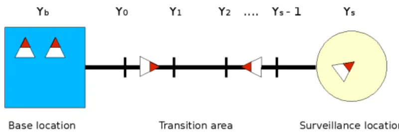
This section provides an overview of the persistent surveillance problem formulation first pro-posed by Bethke et al.19 In the persistent surveillance problem, there is a group of n UAVs equipped with cameras or other types of sensors. The UAVs are initially located at a base location, which is separated by some (possibly large) distance from the surveillance location. The objective of the problem is to maintain a specified number r of requested UAVs over the surveillance location at all times. Figure 1 shows the layout of the mission, where the base location is denoted by Yb, the surveillance location is denoted by Ys, and a discretized set of intermediate locations are denoted by {Y0, . . . , Ys− 1}. Vehicles, shown as triangles, can move between adjacent locations at a rate of one unit per time step.

The UAV vehicle dynamics provide a number of interesting health management aspects to the problem. In particular, management of fuel is an important concern in extended-duration missions such as the persistent surveillance problem. The UAVs have a specified maximum fuel capacity Fmax, and we assume that the rate ˙Fburn at which they burn fuel may vary randomly during the mission due to aggressive maneuvering that may be required for short time periods, engine wear and tear, adverse environmental conditions, damage sustained during flight, etc. Thus, the total

(4)

Figure 1: Persistent surveillance problem

flight time each vehicle achieves on a given flight is a random variable, and this uncertainty must be accounted for in the problem. If a vehicle runs out of fuel while in flight, it crashes and is lost. The vehicles can refuel (at a rate ˙Fref uel) by returning to the base location.

II.A. MDP Formulation

Given the qualitative description of the persistent surveillance problem, an MDP can now be formulated. The MDP is specified by (S, A, P, g), where S is the state space, A is the action space, Pxy(u) gives the transition probability from state x to state y under action u, and g(x, u) gives the cost of taking action u in state x. Future costs are discounted by a factor 0 < α < 1. A policy of the MDP is denoted by µ : S → A. Given the MDP specification, the problem is to minimize the so-called cost-to-go function Jµ over the set of admissible policies Π:

min µ∈ΠJµ(x0) = minµ∈ΠE "_∞ X k=0 αkg(xk, µ(xk)) # .

II.A.1. State Space S

The state of each UAV is given by two scalar variables describing the vehicle’s flight status and fuel remaining. The flight status yi describes the UAV location,

yi∈ {Yb, Y0, Y1, . . . , Ys, Yc}

where Yb is the base location, Ysis the surveillance location, {Y0, Y1, . . . , Ys−1} are transition states between the base and surveillance locations (capturing the fact that it takes finite time to fly between the two locations), and Yc is a special state denoting that the vehicle has crashed.

Similarly, the fuel state fi is described by a discrete set of possible fuel quantities, fi∈ {0, ∆f, 2∆f, . . . , Fmax− ∆f, Fmax}

where ∆f is an appropriate discrete fuel quantity. The total system state vector x is thus given by the states yi and fi for each UAV, along with r, the number of requested vehicles:

x = (y1, y2, . . . , yn; f1, f2, . . . , fn; r)T II.A.2. Control Space A

(5)

• If y_i ∈ {Y₀, . . . , Ys− 1}, then the vehicle is in the transition area and may either move away from base or toward base: ui∈ {“ + ”, “ − ”}

• If y_i = Yc, then the vehicle has crashed and no action for that vehicle can be taken: ui= ∅ • If yi = Yb, then the vehicle is at base and may either take off or remain at base: ui ∈ {“take

off”,“remain at base”}

• If y_i = Ys, then the vehicle is at the surveillance location and may loiter there or move toward base: ui ∈ {“loiter”,“ − ”}

The full control vector u is thus given by the controls for each UAV:

u = (u1, . . . , un)T (1)

II.A.3. State Transition Model P

The state transition model P captures the qualitative description of the dynamics given at the start of this section. The model can be partitioned into dynamics for each individual UAV.

The dynamics for the flight status yi are described by the following rules:

• If yi ∈ {Y0, . . . , Ys− 1}, then the UAV moves one unit away from or toward base as specified by the action ui ∈ {“ + ”, “ − ”}.

• If yi = Yc, then the vehicle has crashed and remains in the crashed state forever afterward. • If y_i = Yb, then the UAV remains at the base location if the action “remain at base” is

selected. If the action “take off” is selected, it moves to state Y0.

• If y_i = Ys, then if the action “loiter” is selected, the UAV remains at the surveillance location. Otherwise, if the action “−” is selected, it moves one unit toward base.

• If at any time the UAV’s fuel level fi reaches zero, the UAV transitions to the crashed state (yi = Yc).

The dynamics for the fuel state fi are described by the following rules: • If y_i = Yb, then fi increases at the rate ˙Fref uel (the vehicle refuels). • If y_i = Yc, then the fuel state remains the same (the vehicle is crashed).

• Otherwise, the vehicle is in a flying state and burns fuel at a stochastically modeled rate: fi decreases by ˙Fburnwith probability pnomand decreases by 2 ˙Fburnwith probability (1 − pnom). II.A.4. Cost Function g

The cost function g(x, u) penalizes three undesirable outcomes in the persistent surveillance mission. First, any gaps in surveillance coverage (i.e. times when fewer vehicles are on station in the surveillance area than were requested) are penalized with a high cost. Second, a small cost is associated with each unit of fuel used. This cost is meant to prevent the system from simply launching every UAV on hand; this approach would certainly result in good surveillance coverage

(6)

but is undesirable from an efficiency standpoint. Finally, a high cost is associated with any vehicle crashes. The cost function can be expressed as

g(x, u) = Clocmax{0, (r − ns(x))} + Ccrashncrashed(x) + Cfnf(x) where:

• ns(x): number of UAVs in surveillance area in state x, • ncrashed(x): number of crashed UAVs in state x, • n_f(x): total number of fuel units burned in state x,

and Cloc, Ccrash, and Cf are the relative costs of loss of coverage events, crashes, and fuel usage, respectively.

Previous work9, 20 presented an adaptation architecture developed for the MDP framework that allowed the system policy to be continually updated online using information from a model estimator. This architecture was shown to reduce the time to successfully estimate the underlying model and compute the updated policy, allowing the system to respond to both initially poor estimates of the model, as well as dynamic changes to the model as the system is running and resulted in improved system performance over non-adaptive approaches.

Figure 2: Representative mission with an embedded adaptation mechanism. The vehicle policy is initialized for an pessimistic set of parameters, but throughout the course of the mission, the model estimator concludes that a more optimistic model is running the system, and the policy is updated with a more appropriate decision to remain at the surveillance location for increased time.

A representative mission with this adaptation embedded is given in Figure 2, with physical vehicle states shown on the left axis and fuel state shown on the right. Vehicle 1 (red) is initialized with a conservative policy (i.e. initial estimate of ˆpnom = 0, while the true value is pnom = 1) and travels from the base location through the intermediate transition area to the surveillance location.

(7)

Due to its pessimistic policy, Vehicle 1 only spends one time step at the surveillance location. However, these initial steps have given Vehicle 1 enough fuel transition observations to update its estimate ˆpnom and form a new policy. These state transitions are made available to all vehicles, which results in Vehicle 2 (blue) remaining on surveillance for one additional time step (for a total of 2 time steps). After only a few “phases” of surveillance plus refueling/waiting, each vehicles’ estimate ˆpnom has converged and the consequent policy results in an increased surveillance time of 4 time steps.

Essentially, this adaptive architecture showed the sensitivity of the policy to changes in the estimated model paramter and provided a feedback mechanism for utilizing updated model esimates in on-line policy generation. These model estimates were updated using passive observations of state transitions and showed improved performance. The focus of this research is to actively seek state transition observations so as to learn the model parameters more quickly and thus leading to better system performance. We approach this focus with uniform and directed exploration strategies, as detailed in SectionIII

III. Integrated Learning with Persistent Surveillance

In this section, we begin by outlining the on-line parameter estimator that runs alongside each of the exploration strategies, providing a means for bilateral comparison between approaches. We then discuss each active learning method in depth and show how it is integrated into the formulation of the Markov decision process via the cost, or reward, function.

III.A. Parameter Estimation

In the context of the persistent surveillance mission described earlier, a reasonable prior for the probability of nominal fuel flow, pnom, is the Beta density (Dirichlet density if the fuel is discretized to 3 or more different burn rates) given by

fB(p | α) = K pα1−1(1 − p)α2−1 (2)

where K is a normalizing constant that ensures fB(p | α) is a proper density, and (α1, α2) are the prior observation counts that we have observed on fuel flow transitions. For example, if 3 nominal transitions and 2 off-nominal transition had been observed, then α1 = 3 and α2 = 2. The maximum likelihood (ML) estimate of the unknown parameter is given by

ˆ pnom=

α1 α1+ α2

(3) Conjugacy of the Beta distribution with a Bernoulli distribution implies that the updated Beta distribution on the fuel flow transition can be expressed in closed form. If the observation are distributed according to

fM(γ | p) ∝ pγ1−1(1 − p)γ2−1 (4)

where γ1 (and γ2) denote the number of nominal (and off-nominal, respectively) transitions, then the posterior density is given by

(8)

By exploiting the conjugacy properties of the Beta with the Bernoulli distribution, Bayes Rule can be used to update the prior information α1 and α2 by incrementing the counts with each observation, for example

α_i0 = αi+ γi ∀i (6)

Updating the estimate with N = γ1+γ2observations, results in the following Maximum A Posteriori (MAP) estimator MAP: pˆnom= α0₁ α0₁+ α0₂ = α1+ γ1 α1+ α2+ N (7) This MAP is asymptotically unbiased, and we refer to it as the undiscounted estimator in this paper. Recent work20 has shown that probability updates that exploit this conjugacy property for the generalization of the Beta, the Dirichlet distribution, can be slow to responding to changes in the transition probability, and a modified estimator has been proposed that is much more responsive to time-varying probabilities. One of the main results is that the Bayesian updates on the counts α can be expressed as

α0_i = λ αi+ γi ∀i (8)

where λ < 1 is a discounting parameter that effectively fades away older observations. The new, discounted estimator can be constructed as before

Discounted MAP: pˆnom=

λα1+ γ1 λ(α1+ α2) + N

(9) As seen from the formulation above, only those state transitions that offer a glimpse of the fuel dynamics can influence the parameter estimator. In other words, only those transitions where the vehicle actually consumes fuel can affect the counts for nominal and off-nominal fuel use (α1 and α2 respectively) and therefore affect the estimate of pnom. For example, transitions from any state to crashed, ∗ → Yc, or from base to base, Yb → Yb, are not modeled as consuming fuel and therefore do not affect the estimate. We therefore introduce the notion of influential state transitions as those that consume fuel and thereby offer a glimpse of the fuel dynamics. For this paper, this notion holds similarly for observations of state transitions and is used interchangeably.

III.B. No Exploration

For the case when no exploration is explicitly encouraged, the only state transitions to occur are those in support of minimizing the loss-of-coverage and/or the probability of crashing, since the objective function remains as originally posed in SectionII.A.4, namely

g(x, u) = Clocmax{0, (r − ns(x))} + Ccrashncrashed(x) + Cfnf(x) (10) where ns(x) is the number of UAVs in surveillance area in state x, ncrashed(x) represents the number of crashed UAVs in state x, nf(x) denotes the total number of fuel units burned in state x, and Cloc, Ccrash, and Cf are the relative costs of loss of coverage events, crashes, and fuel usage, respectively. We expect from this formulation a similar behavior as shown in Figure 2, where the vehicles exhibit a “phasing” behavior, meaning they switch between the surveillance location, Ys, and base, Yb. Additionally, we expect the idle vehicle, that is, the vehicle not tasked for surveillance,

(9)

to remain at Yb until needed and therefore provide no additional influential state transitions. This corresponds to a policy where choosing an action always exploits the current information to find the minimum cost rather than choosing an action to improve/extend the current information in the hope that by doing so, lower cost actions will arise (i.e. exploration).

III.C. Uniform Exploration

As implemented in our earlier work,8, 9 passive adaptation can be used to mitigate these effects of uncertainty, and as agents observe fuel transition throughout the mission, the estimate can be updated using Bayes Rule. Alternatively, active exploration11can be explicitly encoded as a new set of high-level decisions available to the agents to speed up the estimation process. In the persistent surveillance framework, this exploration actually has a very appealing feature: we have noted that vehicles that can refuel immediately are frequently left at the base location for longer times in an idle fashion, effectively waiting for the other surveillance vehicles to begin to return to base (see Figure2, for example). Our key idea for the exploration problem relies on taking advantage of this idle state of the refueled UAVs, and use their idle time more proactively, such as to perform small, exploratory actions that can help improve the model estimates by providing additional influential state transition observations that can be shared with the other agents.

To encourage this type of active exploration, one simple approach is to add a reward into the cost function for any action that results in an influential state transition. The new cost function can be written as

g(x, u) = Clocmax{0, (r − ns(x))} + Ccrashncrashed(x) + Cfnf(x) + Cstonsto(x) (11) where Csto represents the cost (in our case, reward) of observing an influential state transition and nsto(x) denotes the number observed at the current stage (nsto(x) ≤ n). The benefits of this approach include:

• Simplicity - simple cost function modification

• Non-augmented state space of size equal to “No Exploration” case • Well suited for time-varying model parameters

The limitations of Uniform Exploration include:

• Does not intelligently choose which transitions to perform when exploring - all are weighted equally

• Exploration is continuous - the benefit of exploration may decay with time, this formulation does not account for this

III.D. Directed Exploration

While vehicle safety is directly accounted for in the system dynamics, the cost function of Equa-tion (11) does not account for errors in the fuel flow probability. This cost function is solved using a Certainty Equivalence-like argument, in which the ML estimate of the model ˆpnom is used to find the optimal policy. However, the substitution of this ML estimate can lead to brittle policies that can result in increased vehicle crashes.

In addition, a drawback associated with uniform exploration is its inability to gauge the infor-mation content of the state transitions resulting from exploration. Since certainly all influential

(10)

state transitions do not affect the estimator equally, which ones influence the estimator in the “best” way? These are the transitions we want the policy to choose when actively exploring. To address this, we embed a ML estimator into the MDP formulation such that the resulting policy will bias exploration toward the influential state transitions that will result in the largest reduction in the expected variance of the ML estimate p_bnom. The resulting cost function is then formed as

g(x, u) = Clocmax{0, (r − ns(x))} + Ccrashncrashed(x) + Cfnf(x) + Cσ2σ2(

b

pnom)(x)

where C_σ2 represents a scalar gain that acts as a knob we can turn to weight exploration, and

σ2(p_bnom)(x) denotes the variance of the model estimate in state x. The variance of the Beta distribution is expressed as

σ2(p_bnom)(x) =

α1(x)α2(x)

(α1(x) + α2(x))2(α1(x) + α2(x) + 1)

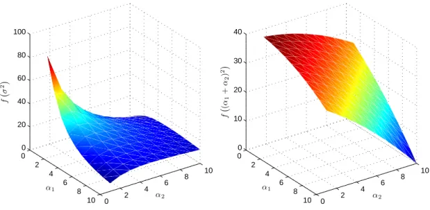
where α1(x) and α2(x) denote the counts of nominal and off-nominal fuel flow transitions in state x respectively, as described in Section III.A. However, in order to justify using a function of α1 and α2 inside the MDP cost function, α1 and α2 need to be part of the state space. Specifically, for each state in the current state space, a set of new states must be added which enumerate all possible combinations of α1 and α2. If we let αi ∈ {1 . . . 10}, this will increase the size of the state space by a factor of 102 . Like many before us, we too curse dimensionality.21 However, all is not lost as we can still produce a policy in a reasonable amount of time (on the order of a couple hours on a decent machine). 0 2 4 6 8 10 0 2 4 6 8 10 0 20 40 60 80 100 α2 α1 f ¡ σ 2 ¢ 0 2 4 6 8 10 0 2 4 6 8 10 0 10 20 30 40 α2 α1 f ¡ (α 1 + α2 ) 2 ¢

Figure 3: Options for the exploration term in the MDP cost function for a directed exploration strategy. (Left) A function of the variance of the Beta distribution parameters α1 and α2. (Right) A quadratic function of α1+ α2.

(11)

Referring now to Figure 3, we see on the left the shape of C_σ2σ2(

b

pnom) for bpnom = f (α1, α2), α1, α2 ∈ {1 . . . 10}. While the variance of the Beta distribution has a significant meaning, the portion of the cost function relating to the variance of the parameter overly favors exploration when αi is small, and too little when αi is large. To remedy this, one could shape a new reward function based also on α1 and α2 that still captures the desired effect of a greater reward (i.e. lower cost) for transitions that lead to a greater reduction in the variance, but perhaps one that does not encode such a drastic difference between these weights. One such possibility is shown on the right-side of Figure 3, where a quadratic function of (α1+ α2) is used.

IV. Simulation Results

In this section, we describe the simulation setup and give various results for each of the explo-ration strategies under the persistent surveillance mission scenario as described in Section I and formulated in Section II. For each approach to exploration, a multi-agent MDP was formulated with 2 agents (n = 2), a crash cost of 50 (Ccrash= 50), a loss-of-coverage cost of 25 (Cloc= 25), a fuel cost of 1 (Cf = 1) and an 80% probability of burning fuel at the nominal rate (pnom = 0.8). In forming the associated cost functions, the exploration term was weighted less than the loss-of-coverage cost, and much less than the cost of a crash. This essentially prioritizes the constraints. The flight status portion of the state is set as yi∈ {Yc, Yb, Y0, Ys}, with a single transition state Y0. The MDP was solved exactly via value iteration with a discount factor α = .9. When simulating the policy, each vehicle was placed initially at base, Yb, with fuel quantity at capacity Fmax.

We organize the results as follows: Section IV.A shows that a vehicle’s fuel capacity directly affects its ability to satisfy any of the objectives in the cost function. In other words, a vehicle with too little fuel will not be able to persistently survey a given location, much less expend additional fuel for the sake of exploration. In SectionIV.B, after getting a feel for the amount of fuel necessary to achieve persistent surveillance, we fix each vehicle’s fuel capacity well above this lower bound and vary the fuel cost to see how each exploration strategy handles a rising cost of fuel. In SectionIV.C, we fix both fuel capacity and cost to see how each exploration strategy affects our estimate of the probability of nominal fuel burn, pnom. Finally, we allow pnom to vary over time in Section IV.C.5 and examine howp_bnom reacts under each exploration strategy.

IV.A. Fuel Capacity

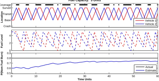
In this section, we search for the minimum fuel capacity needed to persistently observe the surveil-lance location. Since in all cases, exploration is weighted such that loss-of-coverage and crashing are both more important constraints to meet, this minimum provides a lower bound on the fuel capacity needed in order for an exploration strategy to influence on agent behavior. Figure4shows a mission setup where each vehicle can only hold 5 units of fuel. As seen, this is insufficient to maintain persistent coverage of the surveillance area. In addition, Figure 4 shows each vehicle’s location, fuel depletion/replenishment and the overall fuel flow estimate, p_bnom, throughout the mission.

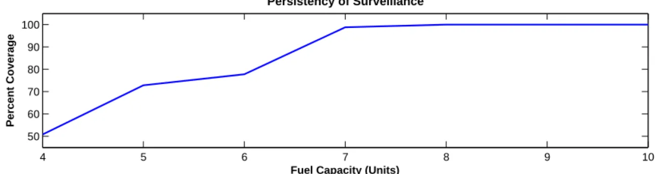
In Figure 5, we compare the persistency of coverage for a handful of vehicle fuel capacities and note that a fuel capacity of less than approximately 8 units is insufficient to achieve the persistent surveillance objective. Therefore, a fuel capacity greater than 8 will allow the vehicle some legroom for exploration. Moving forward, we will fix each vehicle’s fuel capacity at 10 units, giving ample fuel to meet both crash and coverage constraints with enough remaining to engage in exploration

(12)

Crash Base Transit Surveil Coverage Location

Fuel Capacity: 5 Units

Vehicle 1 Vehicle 2 0 2 4 Fuel Level 0 10 20 30 40 50 60 0.5 0.6 0.7 0.8 0.9 Time Units

P(Nom Fuel Burn)

Actual Estimate

Figure 4: Persistent surveillance mission with a fuel capacity of 5 units. As seen, this is insufficient to maintain persistent surveillance.

as each policy dictates.

IV.B. Fuel Cost

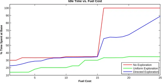
In this section, we increase the cost of fuel and observe how exploration decreases until the cost of using fuel is greater than the cost associated with loss-of-coverage and the vehicle remains at base, Yb for all time. As a metric for exploration, we can measure the amount of time the vehicles spend at base as a function of the cost of fuel for each of the exploration approaches and compare this against the no-exploration case. This curve, averaged over 1000 simulations, is given in Figure 6

and shows that under a no-exploration strategy (red), the time spent at base vs. fuel-cost curve is fairly flat until the threshold is reached where the cost of fuel outweighs the cost of loss-of-coverage. The vehicles then decide to simply remain at base. Under uniform exploration (green), the cost of fuel has a much smaller effect on the amount of time spent at base. This is due to the fact that exploration is set up as a reward, rather than a cost for not exploring, in this formulation. Directed exploration (blue) shows a similar shape as no-exploration, in that a knee appears at the threshold where the cost of coverage (due to fuel use) outweighs the cost of loss-of-coverage. However, the plot is shifted importantly toward less time spent at base and overall shows a balance between the other two approaches.

IV.C. Exploration for Model Learning

In this section, the cost per unit and capacity per vehicle of fuel is fixed at 1 and 10 respectively. We compare the rate at which the model parameter pnom is learned using the MAP model estimator

(13)

4 5 6 7 8 9 10 50 60 70 80 90 100 Persistency of Surveillance Percent Coverage

Fuel Capacity (Units)

Figure 5: Persistent surveillance mission with varying fuel capacity and no exploration strategy. A fuel capacity below 8 units is insufficient to ensure persistent coverage.

given in SectionIII.A. First, we give simulation results for each exploration approach, followed by a Monte-Carlo comparison of the three approaches.

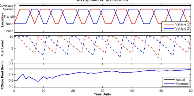
IV.C.1. No Exploration

Under a strategy that does not explicitly encourage exporation, we see the idle vehicle (i.e. the vehicle not tasked with surveillance) remains at the base location until needed, as evidenced in Figure7. This behavior provides influential state transitions due to the active vehicle only (i.e. the vehicle actively surveying) and leads to slow convergence of p_bnom, to pnom.

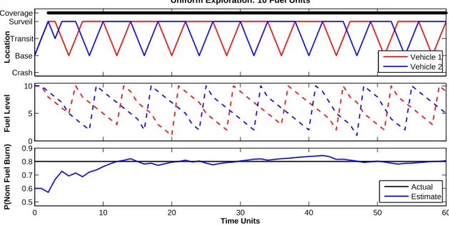
IV.C.2. Uniform Exploration

Essentially, under a uniform exploration strategy, the current stage cost of the MDP is discounted by a set amount when any state transition occurs that results in an observation of the fuel dynamics. This lowered cost effectively encourages an agent to engage in more state transitions when possible. For example, we now see the idle agent leave the base to make additional observations.

In Figure 8, we see that when an agent is given more than enough fuel to achieve persistent surveillance, the idle agent chooses to explore rather than stay at the base location until needed. A particular drawback to uniform exploration is the fact that there is no mechanism to favor specific transitions over others. It is easy to envision a situation where certain state transitions might be more valuable to observe than others, from a learning or estimation perspective. In such a case, transitions whose associated observations are information rich would lead to a reduction in the variance of our estimated, or learned, parameter and should be weighted accordingly.

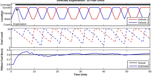
IV.C.3. Directed Exploration

In an effort to address the issues with uniform exploration, we implemented directed exploration strategy that aims to reduce the expected variance ofpbnom via exploration.

In Figure 9, we see that the idle agent immediately leaves base for the sake of exploration, engaging in those transitions that lead to the greatest reduction in the expected variance ofp_bnom. Due to the limited count range for α1 and α2inside the MDP formulation, so that the time required for policy construction is reasonable, the agent only “explores” until the embedded α’s saturate at their upper limits, which for all directed exploration simulations is 10.

(14)

5 10 15 20 25 10 20 30 40 50 60 70 80 90 100

Idle Time vs. Fuel Cost

Fuel Cost

% Time Spent at Base

No Exploration Uniform Exploration Directed Exploration

Figure 6: Persistent surveillance mission where the cost per unit of fuel varies. Under a no-exploration strategy (red), the time-at-base vs. fuel-cost curve is flat until the threshold is reached where fuel cost of persistent coverage outweighs the cost of loss-of-coverage. Under uniform ex-ploration (green), the cost of fuel has relatively little effect as exex-ploration is rewarded in this formulation. Directed exploration (blue) shows a balance between the two extremes.

IV.C.4. Comparison of Exploration Strategies wrt Model Learning

When comparing the exploration strategies with no-exploration and with each other, we calculate several metrics, averaged over 1000 simulation runs. These metrics include: The total number of influential state transitions, total fuel consumed and the total number of vehicles crashed. Table1

summarizes these metrics for each exploration approach.

Table 1: Comparison of averaged results over 1000 simulations

# of Vehicles Crashed 0 0 0

Units of Fuel Consumed 101 115 105

# of Observations 84 96 87

It is interesting to see, in Table 1, that no vehicles crashed under any of the exploration ap-proaches, despite the additional state transition observations provided by the uniform and directed strategies. As this paper is not currently focused on robustness issues, in each case the policy was both constructed and simulated with pnom = 0.8. Thus, the policy accurately dictated vehicle actions to account for this known probability and therefore mitigate vehicle crashes. In addition, all external estimators, as well as the internal estimator in the case of directed exploration, were

(15)

No Exploration: 10 Fuel Units

Actual Estimate

Figure 7: Persistent surveillance mission with 10 units of fuel and no exploration strategy. Fuel is sufficient to achieve persistent coverage of the surveillance location, but fewer state transition observations lead to slower convergence ofp_bnom to pnom.

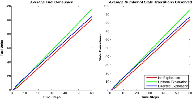
conservatively initialized at pnom= 0.6. This is seen in Figures 7, 8, 9and 11. As for the number of state transitions observed and the amount of fuel consumed, the results confirm the intuition that directed exploration observes fewer transitions and burns less fuel than uniform exploration, but more than no-exploration. The time-history of these numbers are shown in Figure 10 where we see that under a uniform exploration strategy the number of state transitions observed (as well as the closely-related number of fuel units consumed) rises faster than the other strategies and continues at this rate throughout the simulation.

Figure 11 shows the time-history of bpnom under the different exploration strategies and is con-sistent with intuition in that p_bnom converges slowest under no-exploration and both uniform and directed exploration techniques converge slightly faster. The small difference in convergence rate is due to the small number of additional state transitions the uniform and directed strategies gain over no-exploration. Note that under no-exploration, each idle vehicle currently remains at base for only a few time steps before switching roles with the active vehicle. However, as the fuel capacity is increased per vehicle, the idle vehicle will remain at base for longer periods and we therefore expect the difference in the convergence rate of p_bnom between exploration and no-exploration approaches to become greater. This is due to the fact that, under an exploration approach, what was once idle time becomes exploration time to observe influential state transitions and cause the estimator to converge faster.

To verify that as the vehicles are given more fuel the difference in convergence rates of p_bnom between exploration and no-exploration approaches widens, we ran 1000 simulations where each vehicle is given double the amount of fuel as previous (20 units). The results are given in Figure12

(16)

Uniform Exploration: 10 Fuel Units

Actual Estimate

Figure 8: Persistent surveillance mission where each vehicle has 10 units of fuel and implements a uniform exploration strategy with a state transition observation reward of 10. The fundamental change in agent behavior here is that they choose not to stay at base when idle. Rather, the agent’s choose to explore and observe additional state transitions for the sole purpose of learning pnommore quickly.

IV.C.5. Time-Varying Model

We now allow the model parameter pnom to vary with time and compare the results of pbnom for each of the exploration approaches. The results are given in Figure13 and show that none of the approaches as formulated are particularly good at following pnom as it varies over time. We note here that the estimates for each exploration type are generated using the undiscounted estimator presented in SectionIII.A. When the model estimate begins to change, the undiscounted estimator has already seen a handful of state transitions, enough to bring α1 and α2 away from the peaked region of the variance shown in Figure3. Hence, additional observations, regardless of the direction they push the mean, do not influence the mean (likewise the variance) as heavily as the initial observations. Therefore, the estimator is slow to respond to changes over time.

To address this, we implemented a discounted estimator where λ = 0.95, and ran another batch of simulations. The results are given in Figure 14 and show much improvement in the parameter estimate.

V. Conclusions

This paper has extended previous work on persistent multi-UAV missions operating with un-certainty in the model parameters. We have shown that UAV exploratory actions to reduce the parameter uncertainty arise naturally from a modification of the underlying MDP cost function, and

(17)

Directed Exploration: 10 Fuel Units

Actual Estimate Exploration

Figure 9: Persistent surveillance mission where each vehicle has 10 units of fuel and implements a directed exploration strategy with a variance-based cost function and a Beta distribution parameter range of αi ∈ {1 . . . 10}. Exploration is immediate (annotated) as is shortly thereafter not beneficial as the counts internal to the MDP state have reached their threshold of 10.

have shown the value of active learning in improving the convergence speed to the true parameter. We are currently implementing the proposed methodology in our hardware testbed. Our ongoing work is addressing the role of hedging and robustness in the uncertain model. While adaptation is a key component of any dynamic UAV mission, there is a potential risk in simply replacing the uncertain model with the most likely model, even while actively learning. By explicitly accounting for both model robustness and adaptation (both passive and active), safer UAV missions can be performed, mitigating the potential for catastrophic behavior such as vehicle crashes. Another aspect of our research is addressing the role of model consensus across a distributed fleet of UAVs. This problem is of particular relevance to the case when a large fleet of UAVs may lack sufficient connectivity to communicate all their local information to the members of the team. Model con-flict can results in a concon-flicted policy for each agent, and we are investigating methods for reaching agreement across potentially disparate models.

References

1_{Howard, R. A., “Dynamic Programming and Markov Processes,” 1960.} 2

Puterman, M. L., “Markov Decision Processes,” 1994. 3

Littman, M. L., Dean, T. L., and Kaelbling, L. P., “On the complexity of solving Markov decision problems,” In Proc. of the Eleventh International Conference on Uncertainty in Artificial Intelligence, 1995, pp. 394–402.

4

Kaelbling, L. P., Littman, M. L., and Cassandra, A. R., “Planning and acting in partially observable stochastic domains,” Artificial Intelligence, Vol. 101, 1998, pp. 99–134.

5

(18)

0 10 20 30 40 50 60 0 20 40 60 80 100 120

Average Fuel Consumed

Time Steps Fuel Units 0 10 20 30 40 50 60 0 10 20 30 40 50 60 70 80 90 100

Average Number of State Transitions Observed

Time Steps

State Transitions

Figure 10: Comparison of total fuel consumption and total number of influential state transition observations for differing exploration strategies averaging 1000 simulation runs. An influential state transition is one that provides an observation of the vehicle’s fuel dynamics. Note that the two plots are very similar, as fuel consumption and exploration are explicitly connected.

intelligence, Prentice Hall, Upper Saddle River, 2nd ed., 2003.

6_{Iyengar, G., “Robust Dynamic Programming,” Math. Oper. Res., Vol. 30, No. 2, 2005, pp. 257–280.} 7

Nilim, A. and Ghaoui, L. E., “Robust solutions to Markov decision problems with uncertain transition matri-ces,” Operations Research, Vol. 53, No. 5, 2005.

8_{Bertuccelli, L. F., Robust Decision-Making with Model Uncertainty in Aerospace Systems., Ph.D. thesis, MIT,} 2008.

9_{Bertuccelli, B. B. L. F. and How, J. P., “Experimental Demonstration of Adaptive MDP-Based Planning with} Model Uncertainty.” AIAA Guidance Navigation and Control , Honolulu, Hawaii, 2008.

10_{Astrom, K. J. and Wittenmark, B., Adaptive Control , Addison-Wesley Longman Publishing Co., Inc., Boston,} MA, USA, 1994.

11_{Barto, A., Bradtke, S., and Singh., S., “Learning to Act using Real-Time Dynamic Programming.” Artificial} Intelligence, Vol. 72, 2001, pp. 81–138.

12

Kaelbling, L. P., Littman, M. L., and Moore, A. W., “Reinforcement learning: a survey,” Journal of Artificial Intelligence Research, Vol. 4, 1996, pp. 237–285.

13

Gullapalli, V. and Barto., A., “Convergence of Indirect Adaptive Asynchronous Value Iteration Algorithms,” Advances in NIPS , 1994.

14

Moore, A. W. and Atkeson, C. G., “Prioritized sweeping: Reinforcement learning with less data and less time,” Machine Learning , 1993, pp. 103–130.

15

Watkins, C. and Dayan, P., “Q-Learning,” Machine Learning , Vol. 8, 1992, pp. 279–292. 16

Claus, C. and Boutilier, C., “The Dynamics of Reinforcement Learning in Cooperative Multiagent Systems,” AAAI , 1998.

17

Tan, M., “Multi-Agent Reinforcement Learning: Independent vs. Cooperative Learning,” Readings in Agents, edited by M. N. Huhns and M. P. Singh, Morgan Kaufmann, San Francisco, CA, USA, 1997, pp. 487–494.

(19)

18_{Littman, M. L., “Markov games as a framework for multi-agent reinforcement learning,” In Proceedings of the} Eleventh International Conference on Machine Learning , Morgan Kaufmann, 1994, pp. 157–163.

19_{Bethke, B., How, J. P., and Vian, J., “Group Health Management of UAV Teams With Applications to} Persistent Surveillance,” American Control Conference, June 2008, pp. 3145–3150.

20_{Bertuccelli, L. F. and How, J. P., “Estimation of Non-stationary Markov Chain Transition Models.” Conference} on Decision and Control , Cancun, Mexico, 2008.

(20)

0 10 20 30 40 50 60 0.6 0.65 0.7 0.75 0.8

Probability of Nominal Fuel Burn Rate

Time Steps

Actual P(Nom Fuel Burn) No Exploration Uniform Exploration Directed Exploration

Figure 11: Comparison of averaged p_bnom for the differing exploration strategies. Under both exploration types, estimates approach pnom slightly faster than no-exploration due to the idle time steps under the latter being used to provide a few additional observations of vehicle fuel dynamics.

0 10 20 30 40 50 60 0.6 0.65 0.7 0.75 0.8

Time Steps

Figure 12: Comparison of averaged p_bnom when each vehicle is given 20 units of fuel. The no-exploration case has more idle time than for the case of 10 fuel units which again, under both exploration types is used for gaining more glimpses of the vehicle fuel dynamics and causes a slightly faster convergence of p_bnom.

(21)

0 10 20 30 40 50 60 0.6 0.65 0.7 0.75 0.8

Time Steps

Figure 13: Average of 1000 persistent surveillance missions with time-varying model parameter pnom using an undiscounted estimator where additional observations, regardless of the direction they push the mean, do not influence the mean (or variance) as heavily as the initial observations. Therefore, the estimator is slow to respond to changes over time.

0 10 20 30 40 50 60 0.6 0.65 0.7 0.75 0.8

Probability of Nominal Fuel Burn Rate − Discounted Estimator (λ = 0.95)

Time Steps

Figure 14: Average of 1000 persistent surveillance missions with time-varying model parameter pnom and using a discounted estimator, as formulated in SectionIII.A. This results in faster reaction to changes in the model parameter over time.