Control of the space shuttle angle-of-attack during reentry

(1)

Control of the Space Shuttle Angle-of-Attack during Reentry by

Farid Ganji

M.S. Mechanical Engineering, 1994 Sharif University of Technology, Iran

B.S. Mechanical Engineering, 1990 Ferdowsi University of Mashhad, Iran

Submitted to the Department of Mechanical Engineering in Partial Fulfillment of the Requirements for the Degree of

Master of Science in Mechanical Engineering at the

Massachusetts Institute of Technology February 2002

BARKER

ASSACHUSETTS INS IITUTE OF TECHNOLOGY

MAR 2 5

2002

LIBRARIES The author hereby grants to MIT permission to reproduce and to distribute publicly paper and

electronic copies of this thesis document in whole or in part.

:7

Signature of Author...

PEep ment of Ml;hanical Engineering September 10, 2001 Certified by... Rudrapatna V. Ramnath Senior Lecturer Department of Aeronautics and Astronautics Thesis Supervisor A ccepted b y ... ... ...

Ain A. Sonin Chairman, Department Committee on Graduate Students Department of Mechanical Engineering

(2)

Control of the Space Shuttle Angle-of-Attack during Reentry by

Farid Ganji

Submitted to the Department of Mechanical Engineering on September 10, 2001

in Partial Fulfillment of the Requirements for the Degree of Master of Science in Mechanical Engineering

ABSTRACT

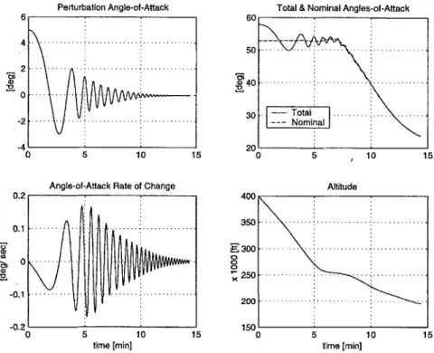
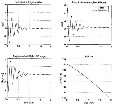
In this study, different approaches to the control of the space shuttle angle-of-attack unwanted oscillations during reentry are presented. The space shuttle glides over a prescribed trajectory that is optimal in that it minimizes the weight of the thermal protection system. The angle-of-attack oscillations are governed by a unified equation that results from the transformation of the equations of motion by means of a change of variable from time to a non-dimensional distance parameter along the trajectory. The original unified equation is modified to be applicable for control purposes and using a generic hypersonic simulation model. The dynamic response obtained by using the generic model shows good agreement with that of the actual space shuttle model. In traversing the earth's atmosphere during reentry, the coefficients of the unified equation vary due to changes in the air density, velocity of the vehicle, flight path angle, nominal angle-of-attack, and aerodynamic characteristics of the space shuttle. The transient response is stable but highly-oscillatory and long-lasting with increasing frequency where it is shown that the die-out time is much longer in the upper atmosphere than that of the lower altitudes. As such, the need for providing the space shuttle orbiter with an angle-of-attack controller is readily justified.

Three different controllers using nonlinear, optimal, and adaptive control methods are developed and simulated. The performance of each controller is analyzed along the upper and lower portions of the trajectory. In both altitude ranges, the controllers eliminate the oscillations and considerably reduce the die-out time. In reducing the time required to achieve the control tasks, the maximum available deflection of the elevator is a major constraint.

The feedback-linearization nonlinear approach proves to be a useful and simple control strategy. Because of its simplicity, the nonlinear controller is employed to characterize the controlled response and calibrate the optimal and adaptive controllers.

In the optimal control approach, a numerical exact solution as well as an analytical approximate solution is developed. The analytical approximate solution is developed through linearizing the Riccati matrix equation and applying the asymptotic multiple time-scales method. The resulting solution for the linearized Riccati matrix is a combination of the elementary harmonic and hyperbolic functions. It is shown that the application of the analytical approximate solution

(3)

considerably reduces the optimal controller computation time. The coefficients and the forcing term in the unified equation vary slowly compared to the highly-oscillatory response of the shuttle to the atmospheric disturbances, regardless of the altitude. It is shown that for the controlled response however, the assumption of slow variations is valid as long as the distance traversed during the control period is small compared to the total distance along the trajectory. Accordingly, it is shown that while the optimal controller using the asymptotic solution performs excellently for lower altitudes, the asymptotic approximation is not applicable in the high-altitude portion of the trajectory.

The parameters appearing in the unified equation are complicated functions of the prescribed trajectory variables and the aerodynamic characteristics of the space shuttle during reentry. As opposed to the nonlinear and optimal controllers, the adaptive controller achieves the control task through a parameter estimation process without using any a priori knowledge of the system parameters. The adaptive controller, as formulated in this study, performs excellently in both upper and lower portions of the trajectory regardless of the level of variations of the aerodynamic and trajectory parameters during the course of control action. It is seen that at lower altitudes, the parameter estimates and the true parameters have the same orders of magnitude which is quite noticeable.

Thesis Supervisor: Rudrapatna V. Ramnath

(4)

ACKNOWLEDGMENTS

I am very grateful that Prof. Ramnath agreed to be my thesis supervisor and provided me with direction and advice during the course of our relationship. I also thank him for choosing a challenging and fascinating thesis topic. I am very appreciative of his supportive efforts and proud of the work that we have done together, and I offer my sincerest thanks to him.

I do not know how to begin to express my gratitude to Prof. Mary Boyce, because it is difficult to quantify the many ways in which she contributed to my development as a graduate student at MIT. She provided me with continual funding, and especially the opportunity to work on a TA project, which allowed me to make a lasting contribution to MIT through the creation of learning-aid desktop experiments that have been and will be used by the institute undergraduates. More importantly, she provided continuous support, guidance, and most significantly, friendship. Her advice and sincere concern was very important during my research and studies. She is an

outstanding mentor and friend who I will not soon forget. I thank her wholeheartedly.

I would like to deeply thank Prof. Sanjay Sarma for believing in me and for his strong and unconditional support, and sincere advice throughout my studies at MIT. I am eternally grateful for his friendship, guidance, and confidence in my abilities.

I am also appreciative to Prof. Lallit Anand that admitted me to the institute and provided me with a wonderful opportunity to contribute to and become enriched by the MIT environment. I would also like to express my sincerest thanks and appreciation to Ms. Leslie Regan for her endless patience, courtesy and assistance throughout my studies at MIT and even before coming to the institute. She always answered my questions and responded to my requests in a professional and thoughtful manner. Although that she is responsible for responding to a large number of students, she always made me feel that she was giving me full consideration, respect and attention.

(8)

NOMENCLATURE

A B CU Cii Cijk CD CL Cm CDO , CL , C,,, CD,, I CL," C, C ,a C M C C D D k e E

f

F g G h H i I J k K L m m, c,k, d,n M1,k, ^ n, c, k, d, ii M = coefficient matrix = coefficient vector

= mean aerodynamic chord of the generic model = coefficients of characteristic Eqs. (4.79) = complex characteristic coefficients

= drag coefficient = lift coefficient

= pitching moment coefficient = nominal aerodynamic coefficients

= aerodynamic stability derivatives = aerodynamic stability derivatives

= elevator effectiveness = drag force

= substitute characteristic coefficients

= base of the natural logarithm = Lyapunov function

= non-dimensional induced disturbance = linear dependence factor

= acceleration due to gravity

= acceleration due to gravity at sea level

= universal gravitational constant = altitude

= constant scaling altitude, Eq. (1.5). Hamiltonian, Eq. (4.12)

= identity matrix

= principal moments of inertia = performance measure

= components of the Riccati matrix

= Riccati matrix

= lift force, Eq. (1.9). Reference length of the space shuttle, Eq. (1.26)

= mass of the space shuttle = true parameters

= estimated parameters = parameter estimation errors

= transformation matrix

= elevator control torque

(9)

N = transformation matrix

PiP2 = components of the co-state vector

P _{= co-state vector, Eq. (4.10). Vector of true parameter, Eq. (5.8)} P' = optimal co-state vector

P = vector of parameter estimates

P = vector of parameter estimation errors

q _{= angular velocity in pitch about the space shuttle center of mass}

= dynamic pressure

Q

= state penalty gain matrix

r _{= radial distance from the Earth center to the space shuttle center of mass}

R = control penalty gain

Re = Earth radius

Rair = gas constant of air

s _{= root of characteristic Eqs. (4.80). Sliding variable, Eq. (5.15)}

Sk = complex characteristic roots

S = reference area

t = time

Tiso = absolute temperature of the isothermal atmosphere

u = control variable

U' = optimal control variable

V = Nominal Velocity

X = state vector

X' = optimal state vector

YM = linear parameterization row vector

z = root of characteristic Eqs. (4.81)

a = perturbation angle-of-attack a- = total angle-of-attack

ao = nominal angle-of-attack

= ratio of the generic model mean chord to the shuttle reference length

= flight path angle

IF = transformation vector, Eq. (4.102). Adaptation gain matrix, Eq. (5.20).

5 = non-dimensional atmospheric mass density

6e = elevator angle

(5e = elevator disturbance control deflection

E = measure of slowness of variations

r/ = slow non-dimensional distance variable

A = characteristic value

A = characteristic functions

A = linearized Riccati matrix p = elevator control coefficient

(10)

60 = nominal pitch angle

V = ratio of moments of inertia

= non-dimensional distance variable

40 = initial non-dimensional distance

4f = final non-dimensional distance

p = atmospheric mass density

PS = atmospheric mass density at sea level

o = inverse non-dimensional pitching moment of inertia

o = time scales

= angular range

0 i= components of the transition matrix

= transition matrix

o , w1 = stiffness and damping coefficients in the unified Eq. (1.38)

920, Qi = coefficient matrices, Eq. (4.46)

Subscripts 0 = nominal value r = radial component = tangential component Re = real part Im = imaginary part x, y, z = stability axes

(11)

INTRODUCTION

This thesis is concerned with the development of different solutions to the control of the space shuttle angle-of-attack oscillations caused mainly by the atmospheric disturbances during reentry. The motivation for doing this investigation stems from the fact that as opposed to the dynamics and stability analysis of the space shuttle during reentry that has been investigated a great deal in the literature such as those done by Vinh and Laitone in [12] and by Ramnath and Sinha in [9], the control aspect of the problem has not been particularly worked on. More specifically, developing an approximate but closed-form solution to the optimal control of the space shuttle angle-of-attack during reentry (Chap. 4) is a novel approach being presented in this thesis. Also, the adaptive controller developed and designed in this thesis (Chap. 5) has its own peculiarities as an application of the adaptive control theory to the reentry problem.

In this investigation., it is assumed that the Earth is spherical, the atmosphere is isothermal, and the shuttle vehicle does not roll. The space shuttle orbiter glides over a prescribed reentry trajectory that is optimal in that it minimizes the weight of the thermal protection system. A realistic generic hypersonic aerodynamic model taken from [3] is used for the computer simulations. The model is a geometrically-simplified hypersonic delta-wing aircraft that has similar aerodynamic characteristics to that of the space shuttle.

Subject to certain conditions, the nonlinear equations of motion and the corresponding kinematic relations are transformed by a change-of-variable, corresponding to the number of scale lengths traversed by the vehicle along the trajectory of the center of mass, to get a unified equation of motion describing the variations of the space shuttle angle-of-attack during reentry [12]. The so called unified equation is a linear second-order inhomogeneous ordinary differential equation with time-varying coefficients.

The coefficients and the forcing term in the unified equation are functions of the prescribed trajectory variables and the aerodynamic characteristics of the space shuttle during reentry. As has been discussed by Ramnath and Sinha in [9], these functions vary slowly along the trajectory as compared to the highly-oscillatory transient response of the space shuttle to angle-of-attack perturbations regardless of the duration of the response. However, it will be shown that for the case of the controlled response, the assumption of slow variation of these parameters is valid as long as the distance traversed during the control period is small compared to the total distance along the reentry trajectory. This is due to the fact that the controlled response is an over-damped non-oscillatory response where its fastness is inversely proportional to the duration of the control action. In fact, the time constant of the controlled response is nearly equal to the duration of control action. It is shown that for the high-altitude portion of the reentry trajectory, the assumption of slow variations is not valid since the space shuttle travels about a quarter of the entire trajectory during the optimal control period.

In this study, three different control approaches are investigated and applied to the unified angle-of-attack equation. In the case of the optimal controller, the control law and the corresponding controlled response of the space shuttle are obtained using both numerical and analytical solutions.

(12)

Practically, the space shuttle orbiter is classified as a long-range hypervelocity vehicle designed for atmospheric as well as extra-atmospheric flights [11]. A typical long-range trajectory with atmospheric and extra-atmospheric portions is illustrated in Fig. 1. The flight is assumed to take place in the plane containing the great circle arc, between the launch point and the landing point. The entire flight is thought of in two phases as described below.

(a) The powered phase in which sufficient kinetic energy provided by the propulsion system is imparted to the vehicle to bring it, under proper guidance, to a prescribed position and velocity in space. The trajectory followed is the arc AB in Fig. 1. The point B is referred to as the burnout position. The powered phase is generally short in terms of both duration and length compared to those of the entire trajectory.

(b) The unpowered phase in which the vehicle travels to its destination under the influence of the gravity and aerodynamic forces. The trajectory followed is the arc BC. For long-range flights like that of the space shuttle orbiter, the total energy imparted to the vehicle at the burnout position B is sufficiently high, with a proper orientation of the burnout velocity, the trajectory followed will have a long portion entirely outside the dense layer of the atmosphere. This portion of the trajectory which is a Keplerian conic is represented by the arc BE in Fig. 1. This is one of the most interesting features in hypersonic flight. For long-range operation, hypervelocity vehicles reduce the cost in fuel consumption since the range XB -XE can be made infinite with

finite energy input. This basic idea led to the concept of present-day shuttle vehicles where, after the powered phase, the subsequent trajectory is entirely flown outside the atmosphere for several days and the required mission is accomplished without additional energy input. When it comes time to return to the Earth, a rocket may be fired to deflect the trajectory such that it intersects the atmosphere of the Earth at a certain point E called the entry position (Fig. 1). This point E is assumed to be at the top of the sensible atmosphere. The subsequent trajectory is called the reentry trajectory. This portion of the trajectory is illustrated by the arc EC in Fig. 1. In this

study, we shall be concerned with the reentry portion of the space shuttle flight.

B

ATMOSPHERE

:-A XB _XE _C

Fig. 1 Typical complete trajectory of long-range hypervelocity vehicles, taken from [11]

In Chapter 1, the longitudinal dynamic equations of motion of the space shuttle orbiter during atmospheric reentry glide are derived, following by the derivation of the unified perturbation

(13)

angle-of-attack equation describing the angle-of-attack oscillations about its prescribed trajectory values. It is assumed that the planet is spherical, the atmosphere is isothermal, and the shuttle vehicle experiences lift and does not roll.

The oscillations of the space shuttle angle-of-attack during reentry have been shown by Vinh and Laitone in [12] to be governed by a second-order inhomogeneous linear differential equation with variable coefficients. This so called unified equation results from the transformation of the nonlinear equations of motion by using a change of independent variable from time to a non-dimensional distance parameter along the trajectory. In this study, the original unified equation is modified to be applicable for control purposes and using the abovementioned generic hypersonic model. In traversing the earth's atmosphere during reentry, variations in the coefficients of the unified equation are due to changes in air density, velocity of the vehicle, flight path angle, nominal angle-of-attack, and the aerodynamic characteristics of the space shuttle vehicle. However, the aerodynamic stability and control derivatives of the shuttle as a hypersonic vehicle vary only due to variations of the nominal angle-of-attack and velocity along the prescribed trajectory. Of these two variable parameters, the nominal angle-of-attack is the dominant one. In Chapter 2, the dynamic response of the space shuttle to the angle-of-attack perturbations, while traveling along the prescribed optimal reentry trajectory, is discussed. In order to simulate the space shuttle aerodynamic characteristics, a realistic generic hypersonic-aircraft computer-simulation aerodynamic model was used for all the computer-simulations in this thesis. The model is a geometrically-simplified hypersonic delta-wing aircraft that has similar aerodynamic characteristics to those of the space shuttle. The trajectory model that was used in the simulations is an optimal reentry trajectory, designed to minimize the weight of the thermal-protection system (TPS) of the space shuttle SSV 049 [4]. The simulation results in this chapter, for the dynamic response of the shuttle vehicle using the generic aerodynamic model, show good agreement with those of the actual space shuttle model reported in [9].

In Chapter 3, in order to suppress the undesired angle-of-attack oscillations, the nonlinear control method of feedback linearization is implemented [10]. Because of its simplicity, the feedback linearization is used to characterize the controlled response of the shuttle to the angle-of-attack perturbations. The feedback-linearization nonlinear controller, subject to the maximum available elevator-angle constraint, offers realistic estimations for the duration and the corresponding rate of decay of the controlled response that will be helpful to design the controllers discussed in the subsequent chapters. The feedback linearization is easy to implement since as will be seen, we only needed to specify the desired time for control action and check if the maximum demanded elevator angle is available.

In Chapter 4, in order to control the perturbations of the space shuttle angle-of-attack during reentry, an optimal control approach is applied to the state space representation of the unified equation. The underlying scheme is the linear quadratic regulator (LQR) formulation that forms a boundary value problem with the specified initial and final conditions for the state vector [6]. Due to the zero final conditions for the state vector as a special case, the formulation and the corresponding Riccati equation are different from those of the conventional linear regulator methodology. The Riccati equation for this special case is called the Riccati equation of the Lyapunov type [5]. Subsequently, a fully numerical solution is discussed followed by

(14)

development of a completely-analytical solution for the control of the space shuttle angle-of-attack perturbations during reentry.

The numerical solution, that is considered to be exact, is obtained by numerically integrating the Riccati equation backwards, and subsequently, solving the co-state differential equation using forward numerical integration. The analytical solution is developed basically to eliminate the backward and forward numerical integrations from the optimal control solution. The motivation for developing an approximate analytical solution is primarily to reduce the computation time that an optimal controller needs to suppress the unwanted oscillations of the space shuttle during reentry. The fact is that while numerical integration schemes require small stepsize to give acceptable results, the accuracy of analytical solutions is not affected by the evaluation stepsize. In the case of approximate analytical solutions however, there must be a balance between the accuracy of the method versus the computation time. The other reason for developing an asymptotic solution is to gain better mathematical insight into the optimal control approach. In order to develop an asymptotic analytical solution, first the Riccati matrix equation is

linearized by using a rigorous mathematical transformation, and subsequently, an asymptotic analytical solution describing the variations of the linearized Riccati matrix is derived. The asymptotic solution is developed by using the multiple time-scales technique. The analytical solutions to the components of the linearized Riccati matrix appear to be a combination of simple harmonic and hyperbolic functions. In the third step, the co-state first-order matrix differential equation is solved analytically, by using a novel matrix transformation. Eventually, the optimal control law and the corresponding state-vector history are determined by using the solutions for the linearized Riccati matrix and the co-state vector. The performance of the presented asymptotic method is evaluated by comparing the corresponding simulation results and computation time to those of the numerical exact solution.

In Chapter 5, in order to suppress the undesired angle-of-attack oscillations, an adaptive control technique is applied to the unified equation, i.e. the original 2nd-order nonlinear differential equation with variable coefficients for the angle-of-attack perturbations.

The adaptive controller is developed and designed by using the modified adaptive control methodology [10]. The main advantage of the adaptive controllers is that they achieve the control task without using any a priori information about the system parameters and their variations. This fact is of special interest in our problem where the trajectory variables and the

aerodynamic characteristics of the space shuttle vary along the reentry trajectory.

The adaptive controller design problem here is to derive a control law for the elevator deflection, and an estimation law for the parameters without using any a priori information about them, such that the space shuttle regains its nominal trajectory angle-of-attack after being perturbed by external or internal disturbances. This means that the deviation of angle-of-attack from its nominal value and all its derivatives with respect to the independent variable or time must vanish at the end of controller action. Thence, the control problem can be categorized as a tracking problem where the desired trajectory is the origin of the state vector space at each instant, or a positioning problem in which the initial position is the disturbed state and the target position is the origin.

(15)

CHAPTER

1 LONGITUDINAL DYNAMICS

In this chapter, the longitudinal dynamic equations of motion of the space shuttle orbiter during atmospheric reentry glide are derived, following by the derivation of the unified perturbation angle-of-attack equation describing the angle-of-attack oscillations about its prescribed trajectory values. It is assumed that the planet is spherical, the atmosphere is isothermal, and the shuttle vehicle experiences lift and does not roll. The formulation and treatment are based on the approach as developed by Vinh and Laitone [12], and Ramnath [9].

1.1 Axis SYSTEM

The stability axes coordinate frame shown in Fig.1.1 will be used to derive the equations of motion of the space shuttle during reentry. As shown in the sketch, the axes emanate from the space shuttle center of mass such that the x-axis is always tangential to the instantaneous flight path and the y-axis passes out the right wing. The z-axis is perpendicular to the other two axes following the orthogonal right-hand rule.

D

W

L

FLIG H T PATH

z.

Fig. 1.1 Stability axes, taken from [12]

1.2 ORBITAL AND ATMOSPHERIC PARAMETERS

The gravitational acceleration, g , varies with the altitude and we have

GM

9 = r2 _(1.1)

where G is the universal gravitational constant, Me is the mass of the earth, and r is the radial distance between the centers the Earth and the space shuttle center of mass (Fig. 1.2). Of this distance, the radial distance from the sea level to the shuttle center of mass is the altitude denoted by h. Thus, we have

(1.2)

(16)

where Re is the average radius of Earth.

L

R

0

Fig. 1.2 Orbital parameters, taken from [11]

Multiplying and dividing (1.1) by Re , we can write

s

g 5 Re _r (1.3)

where g, is the acceleration due to gravity at sea level.

The air density, p , of the isothermal atmosphere is also altitude-dependent. Assuming the air to be a perfect gas and for low orbits like that of the space shuttle, the air density can be calculated

with good accuracy by the exponential formula of

P = pse-'" (1.4)

where p, is the air density at sea level, and

H = RairTso (1.5)

9s

is a constant scaling altitude. Rair is the gas constant for air, T,, is the absolute temperature of

the isothermal atmosphere.

1.3 KINEMATIC RELATIONS

The rate of climb or descent of the flight vehicle traveling along its trajectory is related to the

total velocity, V , of the vehicle center of mass and the flight path angle, y , as the following

(17)

where the dot indicates differentiation with respect to time, and this will be the case henceforth. The flight path angle is the slope of the trajectory with respect to the local horizon. It should be noted that in general a constant flight path angle in orbital flights does not mean a straight-line trajectory. In fact, the trajectory curves down towards the planet because ' is measured relative to the local horizon that keeps changing for the aerospace vehicle.

The pitch attitude rate-of-change, is governed by the following relation

- _q V (1.7)

+-cos _y

r

where q is the angular velocity in pitch about the y-axis of the space shuttle, and the second term on the right-hand-side is the absolute value of the angular velocity of the shuttle center of mass around the earth. Note that in (1.7), q can be positive or negative depending on the pitch direction whereas the second term is always positive. It should also be noted that 6 represents the variations in pitch attitude relative to the earth local horizon. For instance, in order to keep a constant attitude relative to Earth on a circular orbit (j = 0 ), the shuttle needs to have a steady rotational adjustment of

V

Rorbit

Note that if the space shuttle is inverted when orbiting the earth, i.e. the z-axis is pointing towards the outer space, then the sign changes such that

V qinvert + orbit

orbit

1.4 FORCES AND MOMENTS

Besides the gravity force, the longitudinal aerodynamic forces and moments acting on, and about the center of mass of a gliding vehicle, consist of the drag force. D, the lift force L, and the pitching moment M. As sketched in Fig. 1.2, the drag force is in the opposite direction of the vehicle velocity vector or parallel to the wind vector and is defined as positive aft. The lift force is defined as positive up and perpendicular to the wind velocity vector as well as the y-axis (Fig. 1.2). The pitching moment is a combination of the aerodynamic restoring and damping moments as well as the aerodynamic control torques and is positive when the corresponding moment vector points in the positive y-direction. Mathematically, we have

D=CD'qS (1.8)

L = CL;S (1.9)

(18)

where q is the dynamic pressure described by

q = pV2(1.11)

2

and CD , CL, and Cm are the drag, lift, and pitching moment coefficients, respectively. The aerodynamic coefficients are dimensionless functions of the flight variables and they carry the signs of their associated forces or moments. It should be reminded that CD is always positive whereas CL and Cm can be positive or negative, depending on the direction of the lift and pitching moment vectors. The parameter S denotes the reference area and C is the wing mean aerodynamic chord of the lifting vehicle.

1.5 EQUATIONS OF MOTION

1.5.1 DRAG EQUATION

The equation of motion along the flight path is as follows

-D-mgsiny=mV (1.12)

where m is the fuel-burnout reentry mass of the space shuttle. Substituting (1.8) into (1.12), we get

S

PSC v 2

- g sin y _(1.13)

2m

that is called the drag equation and governs the variations of the shuttle velocity under the effect of the drag force and the gravity.

1.5.2 LIFT EQUATION

The equation of motion normal to the flight path is the following

Lcosy -Dsiny-mg =my -m(Vcosy) 2

/r

(1.14)

Differentiating (1.6) with respect to time gives

=

V

sin y +V' cos y (1.15)

Substituting (1.15) into (1.14) yields

Lcos y - D sin y -mg =mY sin y + mV'cos y -mV 2

cos 2 _y/r _(1.16)

(19)

-Dsiny-mgsin 2

y = mY sin y Replacing sin2 y by its cosine equivalent, gives

-Dsiny -mg(1-cos 2 _{y)= m# sin y} _(1.17)

Putting (1.17) into (1.16), we obtain

Lcos y = mg cos 2 _{y+mVkcosy -mV} 2 _cos 2 _y/r

that leads to

. L V 2

Vy -- (g--)cos y

m r

and eventually, using (1.9) results in

r pSC LV 2 v2

r= 2m - (g- )cosy _(1.18)

that is called the lift equation and describes the variations in the flight path due to the unbalance of lift and the centrifugal force against the gravity. For circular orbits or flight paths, j and y are both zero, since the gravity minus lift provides the exact amount of centripetal force needed to keep the space vehicle in orbit.

1.5.3 PITCHING MOMENT EQUATION

The equation of rotational motion about the y-axis of the stability coordinate frame attached to the space shuttle center of mass is as follows

M + 3g(IZ - Ij)sin 20 = I.YqM 2r~-I)sn 6I4 (1.19)

where M is the total pitching moment that includes the aerodynamic restoring, damping, and the body flap as well as the elevator-induced control torques. The second term on the left-hand-side is the gravity gradient torque, in which IX and IZ denote the fuel-burnout rolling and yawing principal moments of inertia, respectively. Similarly, on the right-hand side, I, denotes the fuel-burnout pitching moment of inertia.

Note that the pitching moment of inertia is the same in both stability and body axes, whereas the rolling and yawing moments of inertia in the stability axes deviate from their principal values in the body axes depending on the angle-of-attack. However, this effect is negligible in our analysis since the rolling and yawing moments of inertia only affect the gravity gradient torque that is inversely proportional to r, and very small compared to the aerodynamic pitching moment. Substituting (1.10) into (1.19) and rearranging leads to

(20)

PScCmV 2 +(3g - sin 2 (1.20)

21, _2r _I,

that is called the pitching moment equation and represents the evolution of the pitch angle of the space-flight vehicle, traveling through the atmosphere and gravitational field of a planet. The pitching moment equation is the base equation of motion for pitch and angle-of-attack control purposes.

1.6 AERODYNAMIC COEFFIECIENTS

As pointed out earlier, the aerodynamic coefficients vary as the flight variables change. To this

effect, due to the fact that the nominal aerodynamic coefficients and their derivatives along the trajectory are slowly-varying functions of angle-of-attack and Mach number, for small perturbations of angle-of-attack, we can linearize the perturbed aerodynamic coefficients about their nominal trajectory values. When the space shuttle angle-of-attack is perturbed from its nominal value by atmospheric disturbances, we can write

&

=ao +0 _(1.21)

where Z , _{ao, and a denote the total, nominal, and perturbation angles-of-attack respectively.}

Accordingly, the total pitch angle of the space shuttle as the complementary kinematic relation

will be

6 =y + (1.22)

In addition, considering the fact that do << d , using (1.21) we can approximate the pitch attitude rate-of-change in (1.22) and (1.7) as the following

+ (1.23)

As discussed in [12], the perturbed and linearized aerodynamic coefficients can thus be approximated as below

CD = CD + CD, a (1.24)

CL = CL + CLa (1.25)

Cm=CMO + Cmfa + C, ) + Cmq )O+C M Se (1.26)

where L is the overall length of the space shuttle used as the non-dimensionalizing reference

length corresponding to the trajectory model. CDO, C., and Cm represent the nominal

aerodynamic coefficients along the trajectory and they will be discussed in Sec. 2.3.1. The rest of the coefficients in Eqs. (1.24) through (1.26) are the aerodynamic stability and control derivatives that are described as follows

(21)

CD=

acD

[per radian]

Ce

C. = aCm [per radian]

(1.27a-f) a L V Cni = i~ a(V aCm Cm8e = [per radian]

The stability and control derivatives are slowly-varying functions of the angle-of-attack and Mach number and are inputted to the simulations using a generic hypersonic aircraft model data

that will be discussed in the next chapter.

In (1.26) and (1.27f), ' e denotes the required elevator angle to control the angle-of-attack perturbations. It should be reminded that for delta-wing aircrafts including the space shuttle, the term "elevator" refers to the elevator-mode of the- elevons. Elevons are the dual-action wing-mounted aerosurfaces that can be actuated in the elevator or the aileron mode. In the space shuttle reentry flights, depending on the speed ranges, the pitching moment required for pitch trim and forcing the shuttle to fly along the prescribed trajectory is provided by the body flap and/or the speedbrakes, rather than the elevons. The body flap is the predominant longitudinal trim device, while the wing-mounted elevons (in the elevator mode) are used for longitudinal stability augmentation and pitching-disturbance control. A sketch of the space shuttle orbiter, showing the relative size and locations of the its aerosurfaces, is presented in Fig. 1.3.'

Henceforth, since we are only dealing with the longitudinal control where the elevons function as elevators, we will refer to the elevator-mode of the elevons simply as the elevators.

(22)

Rudder/speedbrake panels Right-hand elevons outboard inboard Glove OMS Aft o reaction 45' jets WingBoyfa sweep Left-hand elevons inboard Outboard

Fig. 1.3 Sketch illustrating the aerosurfaces of the space shuttle orbiter, taken from [11]

Finally, it should be noted that the effect of the trajectory-control body-flap or speedbrake

deflections, is accounted for in CM _{, and therefore their deflections and the corresponding}

aerodynamic effectiveness derivatives do not appear explicitly in the perturbation equations.

1.7 UNIFIED ANGLE-OF-ATTACK EQUATION

As derived in the previous section, the following set of coupled nonlinear differential equations, describe the perturbed longitudinal motion of the space shuttle from its prescribed trajectory during reentry.

S

PSCD 2 _- _g sin y _(1.28) 2m .SC LV 2 V 2 V = -(g - 2)cosy _(1.29) 2m r P - C (g ' )sin 2 0 (1.30) 2I, _2r _I,

where the associated perturbation kinematic relations are

(23)

r = V sin; (1.32) and

6=; +aO+0t (1.33)

with a , as the perturbation variable.

In order to derive a unified equation that describes the variations of the space shuttle angle-of-attack for all possible reentries, as suggested by Laitone in [12], we can use the following universal time transformation

S a(t)= L fJV(t)dt _(1.34)

or equivalently 0

L (t) = V(t) (1.35)

that replaces the real time t by the non-dimensional variable 4 which represents the number of reference lengths L, traveled by the space shuttle center of mass along the trajectory. The following relationships hold -accordingly

d Vd

dt LdU (1.36)

d 2 V 2 d 2 VV' d

dt2 L d) 2

2 _-[]

(1.37)

Henceforth, to show differentiation with respect to (, we will use the following notation that is more convenient

d di

The elimination of 6 and q from the equations of motion as well as the kinematic relations, and change of the independent variable from t to 4, leads to the following non-dimensional second-order nonlinear inhomogeneous differential equation with variable coefficients that describes the variations in the space shuttle angle-of-attack once perturbed from its nominal trajectory values.

a"+ cO(D)a'+ W0(4)a =

f

(4) (1.38)

The corresponding coefficients are

V'

m(l() =mS[ C L/ m+ CM V _(1.39)

gL L

co₀(g) S(3O-C,,-L sin y)CL2 _La

+ D()+ CD

3L gL

(24)

I3Lm v2 Lmo 45C LI'80CM

f 9(v= 2 ACD) 0 - (1- )]cosy+5( H L siny+ c )+62c fll+ CD₀)

-(p)[(+ _ 2)sin 2y+-Lv sin 2(y+ ) (1.41)

and

,U( )= -pO (4)C

(')

(1.42)

Equation (1.38) is called "the unified angle-of-attack equation". Henceforth, we will call w(s),

co0(i), andp(4), as the damping coefficient, the stiffness coefficient, and the control coefficient, respectively. The term f(4) will be referred to as the disturbance term. In order to simplify the derivations and the resulting expressions of the unified equation, the following non-dimensional parameters have also been introduced.

C (1.43) pSL 2m (1.44) I, - I V ~ IY _(1.45) mL2 - - _(1.46)

where 6 serves as the matching parameter between the generic hypersonic-aircraft aerodynamic model and the trajectory model for the actual space shuttle, is the varying non-dimensional air density, v is the ratio of the moments of inertia of the space shuttle in the stability axes, and considered to be invariant, and o is a constant that can be regarded as the inverse non-dimensional pitching moment of inertia of the space shuttle.

It should be reminded that the unified equation (1.38) is nonlinear due to its inhomogeneity that stems from the presence of the inherently-induced forcing term, f(4), on the right-hand side. Physically speaking, considering the equation (1.38) as the representation of a dynamical system, we can see that the relationship between the input, i.e. the elevator angle, and the output, i.e. the angle-of-attack, is not linear.

It is also notable that the parameters oil, w , f , and p , are solely functions of the aerodynamic coefficients and the nominal trajectory variables where they can be evaluated explicitly, if the trajectory flown by the center of mass of the shuttle vehicle is known. This assumes the so-called "limited problem" hypothesis that is the angle-of-attack perturbations have negligible effect on the trajectory.

(25)

The gravitational acceleration gradient, g'(4), and the non-dimensional air density gradient, J'(4), have also been used in the derivation of (1.38), where they are determined as follows. For the gravity gradient, we begin with (1.3)

R2

g = g, --2

r

and differentiate with respect to , to get

' dg - gR( 2r') = -2( )g, = -2( )g (1.47)

d r r r r

However, by applying (1.36) to (1.32) we get

r =-= Lsin y _(1.48)

V

Substituting (1.48) into (1.47), we obtain the gravity gradient as

L

g= -2g( -)sin y (1.49)

For the non-dimensional air density gradient, by differentiating (1.44) we get _' p'SL

2m and from (1.4), we can write

,h'

P ~ P _(1.50)

However, since the Earth radius is constant, we have

h' r' (1.51)

Using (1.51) and substituting (1.48) into (1.50), we can write , L . p= psmyr H and consequently L 5 -(5 L-sin y _(1.52) H

The angular range,

#,

can be computed as is described below. Breaking the velocity vector of the shuttle into the radial and tangential (or orbital) components, we can write

(26)

where

V, = r=V siny (1.53)

V,= = V cos y (1.54)

Considering the orbital component, by rearranging (1.54), we get

= -cos y

r

and using (1.36), we can write

,L

01= -cos Y _(1.55)

r

Finally, integrating (1.55) along the trajectory with respect to 4 , yields

#(

) = L d _(1.56)

fr

0

where y and r are both functions of .

The elapsed time for the shuttle traveling along the trajectory, can be computed at each position by inverting the transformation (1.35) to get

t(f)= L V(d) _(1.57)

0 V( )

1.8 ELEVATOR CONTROL TORQUE

The aerodynamic pitching torque exerted on the space shuttle due to the elevator actuation, i.e. the elevator control torque, can be determined as described below. Using Eqs. (1.10) and (1.26), we can write

M'5'(4) = C1e (e),(4)q )SW (1.58)

Implementing the non-dimensional parameters introduced in Sec. 1.7, we arrive at the following relation for the elevator control torque

Mg,

(5)=

_{la()Cm ()e} _()I,( ₎₂

(1.59) or simply

(27)

CHAPTER 2

DYNAMIC RESPONSE

The dynamic response of the space shuttle to the angle-of-attack perturbations, while traveling along the prescribed optimal reentry trajectory, is discussed in this chapter. In order to simulate the space shuttle aerodynamic characteristics, a realistic generic hypersonic-aircraft computer-simulation aerodynamic model was used for all the computer-simulations in this thesis. The model is a geometrically-simplified hypersonic delta-wing aircraft that has similar aerodynamic characteristics to those of the space shuttle. The trajectory model that was used in the simulations is an optimal reentry trajectory, designed to minimize the weight of the thermal-protection system (TPS) of the space shuttle SSV 049 [4]. The simulation results in this chapter, for the dynamic response of the shuttle vehicle using the generic aerodynamic model, show good agreement with those of the actual space shuttle model reported in [9].

2.1 MODEL GEOMETRY

The space shuttle actual geometry, taken from [1], is shown below. Note that the scale length is in inches. It should be mentioned that the overall length of the shuttle (L = 107.75 ft. or 1293 in.)

was still used as the reference length for deriving the unified equation of the angle-of-attack oscillations, Eq. (1.38), because the available trajectory data to be used for simulations are based on the actual model.

450

XC

Plan area= 560,000 in2

xc =x0 = 840.7 in

L =1293 in (measured from nose to

body flap hinge line)

(28)

A sketch of the generic hypersonic aircraft model used for the simulations in this study is illustrated in Fig. 2.2.

Fig. 2.2 Geometry of the generic hypersonic computer simulation aerodynamic model, taken from [3]

The model geometry is built up of simple geometric shapes in order to simplify the analysis required to estimate the mass properties [3]. The primary structure is modeled as a cylinder 20 ft. in diameter and 120 ft. long. This comprises the volume required for tankage of the liquid hydrogen. Onto this cylinder is attached a pair of 10-degree cones to form the vehicle nose and boattail. This assembly completes the fuselage.

The wings and vertical tail are modeled as thin triangular plates. The mid-wing configuration has been chosen and no dihedral has been added to the wings. The engine module is wrapped around the lower surface of the fuselage and strakes have been extended behind the wings to form the end plates of the half nozzle formed by the lower half of the boattail.

The geometric aerodynamic reference parameters are as follows

Plan Area, S = 6000ft2

Mean Aerodynamic Chord, C = 75ft Span, b = 80ft

(29)

2.2 MASS PROPERTIES

The mass properties of this class of hypersonic vehicles are assumed to be of the same order of magnitude as current supersonic cruise aircraft. The estimate contained in this model has been derived from the XB-70. The take off gross weight is estimated to be in the neighborhood of 300,000 pounds. Of this the fuel (liquid hydrogen) is assumed to comprise 60% (180,000 pounds), and hence the fuel-burnout gliding reentry mass can be approximated by the remaining 40% (120,000 pounds) divided by the acceleration due to gravity at sea level. Therefore

Reentry Mass, m = 3,725 slugs

Rolling Moment of Inertia, IX = 0.87 x 106 slug -

ft

2

Pitching Moment of Inertia, I, = 14.2 x106 _slug-ft2 Yawing Moment of Inertia, IZ = 14.9 x 106 slug -

ft

2

Yaw-Roll Product of Inertia, IX = 0.28 x106 slug -

ft

2

The mass moments of inertia have been estimated from simple geometric solids and shells which approximated the configuration of the model.

2.3 REENTRY TRAJECTORY MODEL

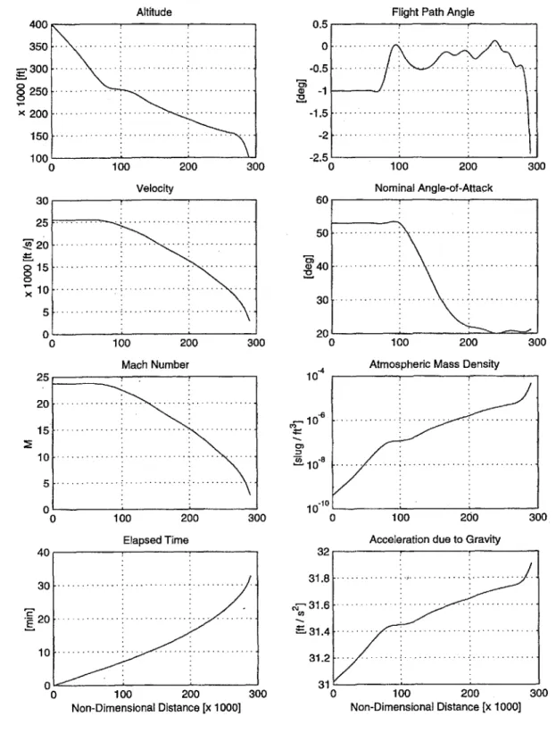
The trajectory model and data used for simulations is an optimal reentry trajectory designed to minimize the thermal-protection system (TPS) weight for the space shuttle SSV 049 [4]. The trajectory characteristics are shown in Fig. 2.3. As can be realized from the flight-path angle history, this reentry model can be classified as a shallow glide entry. The altitude ranges from 400,000 ft at the fringe of atmosphere down to the 100,000 ft where accordingly, the atmospheric density increases about 5 orders of magnitude over the altitude range. The shuttle velocity ranges from Mach 24 in the hypersonic regime down to about Mach 2 in the supersonic range. The total entry time is about 35 minutes and the total distance traveled by the space shuttle along the trajectory is around 6000 miles. The reentry starts with very high angles-of-attack of about 530 in order to maximize the drag and ends at much lower values of around 20*.

(30)

Flight Path Angle 100 200 3C Velocity 0) ci) ~0 0.5 0 -0.5 -1 -1.5 -2 -2.5 C 400 350 300 250 x 200 150 100 C 30 25 20 15 0 10 5 0 30 00 100 200 300 0 Mach Number 100 200 30 Elapsed Time 100 200 Non-Dimensional Distance [x 1000] CO) 10-6 10"8 0 300 10-10 0 32 31.8 ,31.6 31.4 31.2 31 C 100 200 Nominal Angle-of-Attack 100 Atmospheric 200 Mass Density 300 300 100 200

Acceleration due to Gravity

100 200

Non-Dimensional Distance [x 1000]

3

Fig. 2.3 The space shuttle prescribed reentry trajectory characteristics

60 50 40 0 20 15 10 5 01 0 40 30 -20 10 0 C 0 00 3 - . --- - - - -- - -- - - -- -. - -- --.- -. :.. . . . . .. . . .. . . ..:.

--

- -- -- - --

.-.-

--.

-

---..-

---

.

- . -

...

-.

--- ---

..

.

-

.

-..

...

--- -- ---.-.-.-.--

...

----

.-

.

..- - - -- --.. .-.-.-.-- - -- - -- .- - .- - - ..- -- .-.---- ----.. ----. ----.-..---Altitude .- - - -- - - . ....- - -- ---..

---- ---

--

---.---.. ---. ----. ---.----.

--.. ---. ---.-.

--.

--- --- --- --- - ..- -.- . . . .. . .-.-- -- - - - -- - -.- .- . -.-- - - -- - -- - -- -- -- - -- -. - - - -. - - - --

-.

- - - -- - --- -- - --- . ---... -... ---- .-

---

-.

.. .

-

-.

- - ---

...

....-

-.

---

...

-

-.

..

---.-.-- -

..

--

.--

.-

-- ---.-.-.--.-.---.-.--- - - .. .. .- -- - --.-- - .- - .- .- .- .- -- - -- --. --- ----. -. -- - -.- --.-.- -.-.-.- -0 .. ~~~~~~~~~~~~~~~ . -- .- - - .. ...- - - -..- - - --- - - - --- - - - -. - - - -- -- --- -- -- - - -- -....-

---.

-.

---.--

-.-- --.- -

..-.--

.

.--- -. .. .. .--. ---.-.-.-- ---- - .-.- ---..- - .---- ..- --- . .-- ---- . .-- -- .- . .- - .-...- -----. .. .-----. --.-- .. ..- --.-.-- -.. . ... - - - - --. ..-. . . . .- - - .- -... .... ... .. ... ...% ...

...

..

.

(31)

2.3.1 _{NOMINAL AERODYNAMIC COEFFICIENTS ALONG THE TRAJECTORY}

As mentioned before, the unified equation is the governing equation for the angle-of-attack perturbations from the nominal conditions along the prescribed trajectory. Therefore, to analyze and control the angle-of-attack oscillations, we need to know the characteristics of the trajectory flown by the space shuttle. These characteristics include the history of variations of the nominal drag, lift, and pitching moment coefficients along the trajectory, as well as altitude, velocity, flight path angle, and angle-of-attack. For this thesis, since only the latter four variables were available from [9] for the trajectory of interest (Fig. 2.3), the first three variables had to be found by other means.

The nominal drag and lift coefficients can be readily found from the following well-known hypersonic aerodynamic relations as functions of the nominal angle-of-attack [1]

CD = 2sin 3 ao (2.1)

and lift-to-drag ratio is C4 = 2 sin cos a (2.2)

-ift

_ C4 _{= cot a}

(2.3)

Drag _CDO

The nominal pitching moment coefficient, however, should be extracted from the equations of motion and the kinematical relations. The procedure is as the following.

Consider the original unperturbed pitching moment equation with the embedded pitching moment coefficient at its nominal value, along with the kinematic relations below

PSCmV 2 3( ,- -* ( ) )sin 200 (2.4) 2I, _2r _I, V O =q+-cos y _(2.5) r = V sin 2 (2.6) 60 = + ao (2.7)

Applying the time transformation of (1.35) and using the previously-introduced non-dimensional parameters, we get

q' = &c( -)C, _{-- 3g (-)v sin 200} _(2.8)

V , V

-60 = q +--cosr _(2.9)

(32)

6' = a'+a' (2.10)

r' L sin _(2.11)

Solving (2.8) for CM0 , we obtain

Cm = )[q'+ -()v sin 200] _(2.12)

6 V 2r V

As can be seen, the expression for Cm has the term q' that should be expressed in terms of the other available trajectory variables. To this effect, let us solve the first kinematical relation for q and substitute for 6' from (2.10) to get

q

=--(r

+ao) -- cos y

L r

Differentiating with respect to 4 and substituting for r' from (2.11), yields

V V', V' L V

q = -(y' + ao")+-(y + a') -- cos y + (rcos y + y')-sin y (2.13) Finally, substitution for q' from (2.13) into (2.12), results in

I

LV' L 2 V' L L2

3gL

2

Cm - + ao") 2 ('+a')-(

)

-cos y +(-cos y+ y')-sin y +-(-) _{v sin 200]}

5v V r r rV 2rV

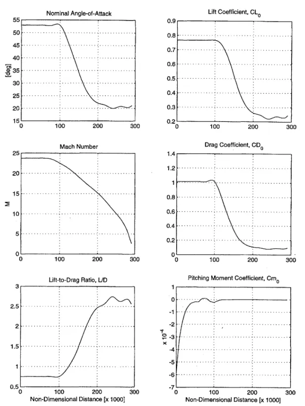
(2.14) where all the variables on the right-hand side are available or computable from the trajectory information in hand. However, note that V', y' and a' as well as y" and a" must be computed by applying a numerical differentiation scheme once and/or twice to the velocity, flight path angle, and angle-of-attack data of the trajectory. Fig. 2.4 shows the computed results. It should be noted that in general, airspeeds above Mach 5 are considered hypersonic, and as can be seen from the nominal Mach number history, most part of the reentry trajectory under consideration falls into the hypersonic regime where the formulas for the drag and lift coefficients, Eqs. (2.1) and (2.2), are valid.

(33)

Nominal Angle-of-Attack .- --- .---.---.----. . -.. -.-.-. . -. -.--. --.. .. . -----. . .---. -. -- . . .. . .---. -.-.-- -.- - - .- .-.- - --- .- --- - --.- --. -.- .- - --.- --. . .. . .-. -.- -. --.-- - -.-- . .. . .-- - - .- ..---..---.---.----.--.---.-. . .-- - ..- -- . ----. . -. -.-. ----. . --0 100 200 300 Mach Number 0 100 200 30 Lift-to-Drag Ratio, UD 100 200 Non-Dimensional Distance [x 1000] 0.9 0.8 0.7 0.6 0.5 0.4 0.3 0.2 1.4 1.2 1 0.8 0.6 0.4 0.2 0 0 100 200 3( Drag Coefficient, CD0 .0 100 200

Pitching Moment Coefficient, Cm₀

100 200 Non-Dimensional Distance [x 1000] 0 0 x 300 1 0 -1 -2 -3 -4 -5 -6 -7 0 0 300 300

Figure 2.4 Nominal aerodynamic coefficients and lift-to-drag ratio during the space shuttle reentry

55 50 45 40 a)35 30 25 20 20-15 10-5 V 2.5 2 1.5 1 0.5 0

Lift Coefficient, CLO

..- .- --- --.-.-- --. -. .-- ----.-- .. .. .- .- - - .- - -- - ..- - -- - -- - - .- ...- - .... .. .- -- -. -.- .. .-.-- .- -.-- -- - - --.-- .- . --. . .. . .- - --.- -.-- - - -- - -- .-- - - -- - --.-- .

----

...

--- --- --

...

..--

--

-

. .- .. --. . .. . .-. - - --...-- . . . .- - - - -.-- - - - -- -- . -. . . .--- -----. ---. ---- --- ---- ---. .-- -. . . .-.-.-- - - --- .-- ---- --- ---.-- .-. . -. ..- ---. - -- ---.. - -- -- - -- --.. -- -- -. -...

-.-.---.---

...

---.-.-- ----

...

.-.--

--

.-

---.

...

--- ---

.

..

.

-. .-.-- - .-.--. .- -- --. --. .-. -. - -- - -..- -- ... ... -- - -- -- - -...- - -.-- .. . .. .-- - - - -- - - - -- - - - .--. -- - .--.- - - - -. . .. . . . - -- -- -- - -- --. . .. . . . . -- - - -- - - -- - - -. -3 ...- - - . .-.- . -. .---. . . .--- -.-- - --- --- -- --- --- --.. .. . -- --. . .. .-- - .-- --.-- .-- ---- .- - ---.- .. ----. . ----. ---

Control of the space shuttle angle-of-attack during reentry

MAR 2 5

2002

CONTENTS

ACKNOWLEDGMENTS

NOMENCLATURE

f

Q

INTRODUCTION

CHAPTER

1

LONGITUDINAL DYNAMICS

D

W

L

z.

S

/r

V

&

acD

S

(1.37)

f

(')

#,

#(

(5)=

CHAPTER 2

ft

ft

ft

--

- -- -- - --

.-.-

--.

-

---..-

---

.

- . -

...

-.

--- ---

..

.

-

.

-..

...

--- -- ---.-.-.-.--

...

----

.-

.

---- ---

--

---.---.. ---. ----. ---.----.

--.. ---. ---.-.

--.

-.

---

-.

.. .

-

-.

- - ---

...

....-

-.

---

...

-

-.

..

---.-.-- -

..

--

.--

.-