INTERACTING BRANCHING PROCESSES AND LINEAR FILE-SHARING NETWORKS

©

Applied Probability Trust 2010

INTERACTING BRANCHING PROCESSES AND LINEAR FILE-SHARING NETWORKS

LASSE LESKELÄ,

Helsinki University of Technology PHILIPPE ROBERT

FLORIAN SIMATOS,

INRIA Paris-Rocquencourt

Abstract

File-sharing networks are distributed systems used to disseminate files among nodes of a communication network. The general simple principle of these systems is that once a node has retrieved a file, it may become a server for this file. In this paper, the capacity of these networks is analyzed with a stochastic model when there is a constant flow of incoming requests for a given file. It is shown that the problem can be solved by analyzing the asymptotic behavior of a class of interacting branching processes. Several results of independent interest concerning these branching processes are derived and then used to study the file-sharing systems.

Keywords: Interacting branching process; peer-to-peer algorithm 2010 Mathematics Subject Classification: Primary 60J80; 60J85

Secondary 90B18

1. Introduction

File-sharing networks are distributed systems used to disseminate information among some nodes of a communication network. The general simple principle is the following: once a node has retrieved a file it becomes a server for this file. An improved version of this principle consists of splitting the original file into several pieces (called ‘chunks’) so that a given node can retrieve simultaneously several chunks of the same file from different servers. In this case, the rate to get a given file may thus increase significantly, as well as the global capacity of the file-sharing system: a node becomes a server of a chunk as soon as it has retrieved it and not only when it has the whole file. These schemes disseminate information efficiently as long as the number of servers grows rapidly.

In this paper we investigate the maximal throughput of these file-sharing networks, i.e.

whether the system can or cannot cope with a constant flow of incoming requests for a given file. Two cases are considered, either the file consists of one chunk or the file is split into two chunks that are retrieved sequentially, which we will refer to as a linear file-sharing network.

It is assumed that arrival times are Poisson and chunk transmission times are exponentially distributed. In this setting, the stability property of the file-sharing system is expressed as

Received 6 July 2009; revision received 16 April 2010.

Work partially supported by the SCALP project funded by the EEC Network of Excellence Euro-FGI, and the Academy of Finland.

∗Current address: Aalto University, Department of Mathematics and Systems Analysis, PO Box 11100, 00076 Aalto, Finland. Email address: lasse.leskela@iki.fi

∗∗Postal address: INRIA Paris-Rocquencourt, Domaine de Voluceau, BP 105, 78153 Le Chesnay, France.

∗∗∗Email address: philippe.robert@inria.fr

∗∗∗∗Email address: florian.simatos@inria.fr

834

λ µ₀x₁

x0 x1

µ₂x₂

x2

νx₂

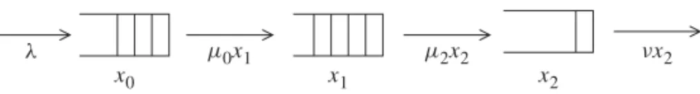
Figure

1: Transition rates outside the boundaries of the file-sharing network with two chunks.

the ergodicity property of the associated Markov process. Even in this simple framework, mathematical studies are quite scarce; see [13], [17], [18], and the references therein.

The main technical difficulty in proving stability/instability results for this class of stochastic networks is that, except for the input, the Markov process has unbounded jump rates, in fact proportional to one of the coordinates of the current state. If x servers have a chunk, since each of them can deliver this chunk, they globally provide this chunk at a rate proportional to x. For this reason, the classical tools related to fluid limits cannot be used easily in this setting. See [4], [5], and [14] for example. However, this class of processes is close to another important class of stochastic processes, namely branching processes, where a population of size x evolves at a rate proportional to x . As will be seen, a file-sharing system that splits files into several chunks can be represented as a Markov process associated to multitype branching processes with interaction.

1.1. Interacting branching processes

Consider the case of a file split into two chunks, and suppose that a new user arriving in the network first requests chunk number 1 and then requests chunk number 2. Assume further that a server of type 1, i.e. having chunk 1 only, distributes it at rate µ

, while a server of type 2, having chunks 1 and 2, distributes only chunk 2 at rate µ

. For i = 0, 1, 2, let X

(t) be the number of type-i servers at time t . A type-0 server is simply a user without any chunk. The crucial observation is that as long as there are requests for chunk i ∈ {1, 2}, then (X

(t)) grows similarly as a branching process where individuals give birth to one child at rate µ

, since each server offers a capacity µ

for the requested chunk. On the other hand, a new arrival in X

corresponds to a departure in X

, since the new type-2 server was a type-1 server; thus deaths in X

are governed by births in X

. See Figure 1.

The file-sharing network under consideration can thus be seen as a system of interacting branching processes where the births and the deaths of individuals are correlated. In the simpler case of one chunk, a description as a branching process (without interaction) has been used to analyze the transient behavior of these file-sharing systems. See [17], [19], and [21].

In Sections 2 and 3 we present results of independent interest concerning branching processes where individuals are killed at the instants (σ

) of a random point process. In Section 2 a criterion for the extinction of the branching process is obtained in terms of the sequence (σ

), and an asymptotic result is derived in this case. In Section 3 we consider the case where (σ

) is the sequence of birth instants of another independent branching process. Several useful estimates are derived in this setting. These results are used to establish the stability results concerning file-sharing systems with two chunks. The stability properties of a network with a single-chunk file are analyzed in detail in Section 4. The case of file-sharing networks with two chunks is detailed in Section 5.

2. Yule processes with killing

A Yule process (Y (t)) with rate µ > 0 is a Markovian branching process with Q-matrix

q

(x, x + 1) = µx for all x ≥ 0. (2.1)

A Yule process is simply a pure-birth process, where each individual gives birth to a child at rate µ.

Yule processes are the basic branching processes that appear in analyzing the two-chunk network of Section 5. Actually, a variant of this stochastic model will be needed, where some individuals are killed. In this section we study this model when killings are given by an exogenous process and occur at fixed (random or deterministic) epochs; in Section 3 killings result from the interaction with another branching process.

In terms of branching processes, this killing procedure amounts to pruning the tree, i.e. to cut some edges of the tree, and the subtree attached to it. This procedure is fairly common for branching processes, in the Crump–Mode–Jagers model for example; see [6]. See also [1]

or [11].

2.1. A Yule process killed at fixed instants

Until the end of this section, it is assumed that, provided that the population is nonempty, at epochs σ

, n ≥ 1, an individual is removed from the population of an ordinary Yule process (Y (t)) with rate µ

starting with Y (0) = w ∈ N individuals. It is assumed that (σ

) is some fixed nondecreasing sequence. It will be shown that the process (W(t)) obtained by killing one individual of (Y (t)) at each of the successive instants (σ

) survives with positive probability when the series with general term (e

) converges.

We define

κ = inf {n ≥ 1 : W(σ

) = 0 }.

The process (W(t)) can be represented by W(t) = Y (t) −

i=1

X

(t) 1

, (2.2)

where, for 1 ≤ i ≤ κ and t ≥ σ

, X

(t) is the total number of children at time t in the original Yule process of the i th individual killed at time σ

. In terms of trees, (W(t)) can be seen as a subtree of (Y (t)) : for 1 ≤ i ≤ κ , (X

(t)) is the subtree of (Y (t)) associated with the i th particle killed at time σ

.

It is easily checked that (X

(t − σ

), t ≥ σ

) is a Yule process starting with one individual and, since a killed individual cannot have one of his descendants killed, that the processes

( X

(t)) = (X

(t + σ

), t ≥ 0 ), 1 ≤ i ≤ κ, are independent Yule processes.

For any process (U(t)), we define

(M

(t)) := (e

U(t)). (2.3)

If ( X(t)) is a Yule process with rate µ

, the martingale (M

(t)) converges almost surely and in L

to a random variable M

(∞) with an exponential distribution with mean X( 0 ) , and, by Doob’s inequality,

E

sup

M

(t)

≤ 2 sup

t≥0

E(M

(t)

) < +∞.

See [3]. Consequently,

e

W(t) = M

(t) −

i=1

e

M

(t − σ

) 1

,

and, for any t ≥ 0,

e

M

(t − σ

) 1

≤

i=1

e

sup

s≥0

M

(s).

Assume now that

i≥1

e

< +∞: then the last expression is integrable, and Lebesgue’s theorem implies that (M

(t)) = ( e

W(t)) converges almost surely and in L

to

M

(∞) = M

(∞) −

e

M

(∞).

Clearly, for some large enough w

and then for any w ≥ w

, we have E

(M

(∞)) ≥ w −

i=1

e

> 0,

in particular P

(M

(∞) > 0 ) > 0 and P

(W(t) ≥ 1 for all t ≥ 0 ) > 0. If Y ( 0 ) = w < w

and σ

> 0, then P

(Y (σ

) ≥ w

+ 1 ) > 0, and, therefore, by translation at time σ

, the same conclusion holds when the sequence ( e

) has a finite sum. The following proposition has thus been proved.

Proposition 2.1. Let (W(t)) be a process growing as a Yule process with rate µ

and for which individuals are killed at nondecreasing instants (σ

) with σ

> 0. If

+∞

i=1

e

< +∞

then as t gets large, and for any w ≥ 1, the variable (e

W(t)) converges P

-almost surely and in L

to a finite random variable M

(∞) such that P

(M

(∞) > 0) > 0.

Proposition 2.1 establishes the minimal results needed in Section 5. However, Kolmogorov’s three-series, see [20, p. 115], can be used in conjunction with Fatou’s lemma to show that (W(t)) dies out almost surely when the series with general term (e

) diverges.

3. Interacting branching processes

In this section we study theYule process of the previous section when killing times correspond to the birth times of some other branching process. The other branching process can be seen as a renewing Bellman–Harris process.

3.1. Renewing Bellman–Harris process

In the rest of this section, µ

, ν > 0 are fixed and (Z(t)) is a birth-and-death process whose Q-matrix, Q

, is given by

q

(z, z + 1) = µ

(z ∨ 1) and q

(z, z − 1) = νz. (3.1)

In the rest of the paper n ∨ m denotes max(n, m) for n, m ∈ N. This process can be

described equivalently as a time-changed M/M/1 queue (see Proposition 3.1) or as a sequence of

independent branching processes (see Proposition 3.2). The time change is the discrete analog

of the Lamperti transform between continuous-state branching processes and Lévy processes;

see [7]. As will be seen, these two viewpoints are complementary.

Let (σ

) be the sequence of birth instants (i.e. positive jumps) of (Z(t)), and let (B

(t)), the corresponding counting process of (σ

), be given by, for t ≥ 0,

B

(t) =

i≥1

1

.

Proposition 3.1. (Queueing representation.) If Z(0) = z ∈ N then

(Z(t), t ≥ 0 ) =

(L(C(t)), t ≥ 0 ), (3.2) where (L(t)) is the process of the number of jobs of an M/M/1 queue with input rate µ

and service rate ν, and with L(0) = z and C(t) = inf{s > 0 : A(s) > t }, where

A(t) =

0

1 1 ∨ L(u) d u.

Proof. It is not difficult to check that the process (M(t)) := (L(C(t))) has the Markov property. Let Q

be its Q-matrix. For z ≥ 0,

P(L(C(h)) = z + 1 | L(0) = z) = µ

E(C(h)) + o(h) = µ

(z ∨ 1)h + o(h);

hence, q

(z, z + 1 ) = µ

(z ∨ 1 ) . Similarly, q

(z, z − 1 ) = νz . The proposition is proved.

Corollary 3.1. For any γ > (µ

− ν) ∨ 0 and z = Z(0) ∈ N, E

n=1

e

< +∞.

Proof. Proposition 3.1 shows that, in particular, the sequences of positive jumps of (Z(t)) and of (L(C(t))) have the same distribution. Hence, if N

= (t

) is the arrival process of the M/M/1 queue, a Poisson process with parameter µ

, then, using the notation of the above proposition, the relation

(σ

) =

(A(t

))

holds. By using standard martingale properties of stochastic integrals with respect to Poisson processes, see [15], we obtain, for t ≥ 0,

E

n≥1

e

= E

0

e

N

( d s)

= µ

E

0

e

ds

= µ

0

e

E

(Z(u) ∨ 1) du, (3.3) where relation (3.2) has been used for the last equality. Kolmogorov’s equation for the process (Z(t)) gives

φ(t) := E

(Z(t))

= µ

0

E

(Z(u) ∨ 1) du − ν

0

E

(Z(u)) du

≤ (µ

− ν)

0

φ(u) du + µ

t ;

therefore, by Gronwall’s lemma, φ(t) ≤ φ(0) + µ

0

ue

du ≤ z + µ

µ

− ν t e

. From (3.3), we conclude that

E

n

e

= E

n

e

< +∞.

The proposition is proved.

Before hitting 0, (Z(t)) can be seen as a Bellman–Harris branching process with Malthusian parameter α = µ

−ν ; see [3]. This Bellman–Harris branching process describes the evolution of a population of independent particles: each particle, at rate λ := µ

+ν , either splits into two particles with probability p := µ

/(µ

+ ν) or dies with probability 1 − p. These processes will be referred to as (p, λ)-branching processes in the sequel.

A (p, λ)-branching process survives with positive probability only when p >

, in which case the probability of extinction is equal to q = (1 − p)/p = ν/µ

. The process (Z(t)) only differs from a (p, λ)-branching process insofar as it regenerates after hitting 0, after a time exponentially distributed. When it regenerates, it again behaves as a (p, λ)-branching process (started with one particle), until it hits 0 again.

Proposition 3.2. (Branching representation.) If Z(0) = z ∈ N and ( Z(t)) is a (p, λ)- branching process started with z ∈ N particles and T its extinction time, then

(Z(t), 0 ≤ t ≤ T ) =

( Z(t), 0 ≤ t ≤ T ), where T = inf{t ≥ 0 : Z(t) = 0} is the hitting time of 0 by (Z(t)).

Corollary 3.2. Suppose that µ

> ν . Then, P

-almost surely for any z ≥ 0, there exists a finite random variable Z(∞) such that

t→+∞

lim e

Z(t) = Z(∞) and Z(∞) > 0.

Proof. When µ

> ν, the process (Z(t)) couples in finite time with a supercritical (p, λ)- branching process ( Z(t)) conditioned on nonextinction; this follows readily from Proposi- tion 3.2 (or see Appendix A for details). Since, for any supercritical (p, λ) -branching process, ( exp (−(µ

− ν)t) Z(t)) converges almost surely to a finite random variable Z(∞) , positive on the event of nonextinction (see [10]), we obtain the desired result.

Due to its technicality, the proof of the following result is postponed to Appendix A; this result is used in the proof of Proposition 3.4.

Proposition 3.3. Suppose that µ

> ν. If η

(x ) = 2 − x − √

x (4 − 3x )

2(1 − x) , 0 < x < 1, (3.4)

then, for any 0 < η < η

(ν/µ

), sup

E

t

sup

(e

B

(t)

)

< +∞.

3.2. A Yule process killed at the birth instants of a renewing Bellman–Harris process We now consider the main interacting branching processes: in addition to (Z(t)), we consider an independent Yule process (Y (t)) with parameter µ

(its Q-matrix is defined by (2.1) with µ = µ

). We proceed similarly as in Section 2: a process (W(t)) is defined by killing one individual of (Y (t)) at each of the birth instants (σ

) of (Z(t)) (see [2] and the references therein for related models). Recall that (W(t)) is given by (2.2). The following results are key to analyzing the two-chunk network of Section 5.

Proposition 3.4. Assume that µ

− ν > µ

, and let H

be the extinction time of (W(t)), i.e.

H

= inf{t ≥ 0 : W(t) = 0}.

Then the random variable H

is almost surely finite and (i) Z(H

) − Z(0) ≤ e

M

, where

M

= sup

t≥0

(e

Y (t)),

(ii) there exists a finite constant C such that, for any z ≥ 0 and w ≥ 1,

E

(H

) ≤ C(log(w) + 1). (3.5)

In (3.5) the subscript (w, z) refers to the initial state of the Markov process (W(t), Z(t)).

More generally, in the rest of the paper we use the convention that if (U(t)) is a Markov process then the index u of P

and E

will refer to the initial condition of this Markov process.

Proof of Proposition 3.4. Define α = µ

− ν . Concerning the almost-sure finiteness of H

, note that (2.2) entails that W(t) ≤ Y (t) − B

(t) for all t ≥ 0 on the event {H

= +∞} . As t goes to ∞, both exp(−µ

t)Y (t) and exp(−αt)B

(t) converge almost surely to positive and finite random variables (see [10]), which implies, when α = µ

− ν > µ

, that W(t) converges to −∞ on {H

= +∞}, and so this event is necessarily of probability 0.

Point (i) of the proposition comes from identity (2.2) evaluated at t = H

:

Z(H

) − Z( 0 ) ≤ B

(H

) ≤ Y (H

) ≤ e

M

. (3.6) By using the relation exp(x) ≥ x, (3.5) follows from the following bound: for any η <

η

(ν/µ

) (recall that η

is given by (3.4)),

w≥

sup

[w

E

(e

)] < +∞. (3.7) So all that is left to prove is this bound. Under P

, (Y (t)) can be represented as the sum of w independent and identically distributed (i.i.d.) Yule processes, and so M

≤ M

+· · ·+ M

with (M

) i.i.d. distributed like M

under P

; inequality (3.6) then entails that

e

≤

i=1

M

t≥σ

sup

e

B

(t)

.

By the independence of (M

) and (B

(t)), Jensen’s inequality gives, for any η < 1, E

(e

) ≤ w

(E(M

))

E

t≥σ

sup

(e

B

(t)

)

;

hence, bound (3.7) follows from Proposition 3.3.

We conclude this section with a Markov chain which will be used in Section 5. Define recursively the sequence (V

) by V

= v and

V

=

A

I

, n ≥ 0, (3.8)

where, for each n, (I

, k ≥ 1) are identically distributed integer-valued random variables independent of V

and A

(V

), and such that E(I

) = p for some p ∈ (0, 1). For v > 0, A

(v) is an independent random variable with the same distribution as Z(H

) under P

, i.e. with the initial condition (W(0), Z(0)) = (1, v).

Equation (3.8) can be interpreted as a branching process with immigration, see [16], or also as an autoregressive model.

Proposition 3.5. Under the condition µ

− ν > µ

, if (V

) is the Markov chain defined by (3.8) and, for K ≥ 0,

N

= inf{n ≥ 0 : V

≤ K}, then there exist γ > 0 and K ∈ N such that

E (N

| V

= v) ≤ 1

γ log ( 1 + v) for all v ≥ 0 . (3.9) The Markov chain (V

) is in particular positive recurrent.

Proof. For V

= v ∈ N, Jensen’s inequality and (3.8) give the relation E

log

1 + V

1 + v

≤ E

log

1 + pZ(H

) 1 + v

. (3.10)

From Proposition 3.4 and by using the same notation, we obtain, under P

, Z(H

) ≤ v + e

M

,

where (Y (t)) is a Yule process starting with one individual. By looking at the birth instants of (Z(t)), it is easily checked that the random variable H

under P

is stochastically bounded by H

under P

. It follows from the integrability of H

under P

(proved in Proposition 3.4) and of M

that the expression

log

1 + p(v + e

M

) 1 + v

bounding the right-hand side of (3.10) is also an integrable random variable under P

. Lebesgue’s theorem therefore gives

lim sup

v→+∞

E

log

1 + V

1 + v

≤ log p < 0.

Consequently, we conclude that v → log(1 + v) is a Lyapunov function for the Markov chain (V

), i.e. if γ = −(log p)/2, there exists K such that, for v ≥ K,

E

log(1 + V

) − log(1 + v) ≤ −γ.

Foster’s criterion, see Theorem 8.6 of [14], implies that (V

) is indeed ergodic and that (3.9)

holds.

4. The single-chunk network

This section is devoted to the study of a class of two-dimensional Markov jump processes (X

(t), X

(t)), with corresponding Q-matrix

given, for x = (x

, x

) ∈ N

, by

⎧ ⎪

⎨

⎪ ⎩

r

[(x

, x

), (x

+ 1, x

)] = λ,

r

[(x

, x

), (x

− 1, x

+ 1)] = µr(x

, x

)(x

∨ 1) 1

,

r

[(x

, x

), (x

, x

− 1 )] = νx

,

(4.1)

where x → r(x ), referred to as the rate function, is some fixed function on N

with values in [ 0 , 1 ] .

From a modeling perspective, this Markov process describes the following system. Requests for a single file arrive at rate λ , the first component X

(t) is the number of requests which did not get the file, whereas the second component is the number of requests having the file and acting as servers until they leave the file-sharing network. The constants µ and ν can be viewed as the file transmission rate and the rate at which servers having the file leave, respectively.

The term r(x

, x

) describes the interaction of downloaders and uploaders in the system. The term x

∨ 1 can be interpreted so that there is one permanent server in the network, which is contacted if there are no other uploader nodes in the system. A related system where there is always one permanent server for the file can be modeled by replacing the term x

∨ 1 by x

+ 1.

See the remark at the end of this section.

Several related examples of this class of models have been recently investigated. The case r(x

, x

) = x

x

+ x

was considered in [9] and [12]; in this case the downloading time of the file is neglected.

Susitaival et al. [18] analyzed the rate function r(x ) , r(x

, x

) = 1 ∧

α x

x

,

where α > 0 and a ∧ b denotes min (a, b) for a , b ∈ R . This model allows us to take into account the fact that a request cannot be served by more than one server. See also [13].

With a slight abuse of notation, for 0 < δ ≤ 1, the matrix

will refer to the case when the function r is identically equal to δ. Note that the boundary condition x

∨ 1 for departures from the first queue prevents the second coordinate from ending up in the absorbing state 0. Other possibilities are discussed at the end of this section. In the following (X

(t)) = (X

(t), X

(t)) and (X

(t)) = (X

(t), X

(t)) will denote Markov processes with Q-matrices

and

, respectively.

4.1. Free process

For δ > 0, Q

denotes the following Q -matrix:

⎧ ⎪

⎨

⎪ ⎩

Q

[(y, z), (y + 1, z)] = λ,

Q

[(y, z), (y − 1, z + 1)] = µδ(z ∨ 1), Q

[(y, z), (y, z − 1)] = νz.

(4.2)

The process (Y

(t)) = (Y

(t), Y

(t)), referred to as the free process, will denote a Markov

process with Q-matrix Q

. Note that the first coordinate (Y

(t)) may become negative. The

second coordinate (Y

(t)) of the free process is the birth-and-death process with the same distribution as the process (Z(t)) introduced in Section 3. It is easily checked that if ρ

defined as δµ/ν is such that ρ

< 1 then (Y

(t)) is an ergodic Markov process converging in distribution to Y

(∞) and

λ

(δ) := ν E(Y

(∞)) = δµ E(Y

(∞) ∨ 1) = δµ

(1 − ρ

)(1 − log(1 − ρ

)) . (4.3) When ρ

> 1, then the process (Y

(t)) converges almost surely and in expectation to ∞. In the sequel, λ

(1) is simply denoted as λ

.

In the following it will be assumed, see condition (4.6) below, that the rate function r converges to 1 as the first coordinate goes to ∞ ; as will be seen, the special case r ≡ 1 then plays a special role, and so before analyzing the stability properties of (X

(t)) , we begin with an informal discussion when the rate function r is identically equal to 1. Since the departure rate from the system is proportional to the number of requests/servers in the second queue, a large number of servers in the second queue gives a high departure rate, irrespectively of the state of the first queue. The input rate of new requests being constant, the real bottleneck with respect to stability is therefore when the first queue is large. The interaction of the two processes (X

(t)) and (X

(t)) is expressed through the indicator function of the set {X

(t) > 0}. The second queue (X

(t)) locally behaves like the birth-and-death process (Y

(t)) as long as (X

(t)) is away from 0. The two cases ρ

> 1 and ρ

< 1 are considered.

If ρ

> 1, i.e. µ > ν, the process (X

(t)) is a transient process as long as the first coordinate is nonzero. Consequently, departures from the second queue occur faster and faster. Since, on the other hand, arrivals occur at a steady rate, departures eventually outpace arrivals. The fact that the second queue grows when (X

(t)) is away from 0 stabilizes the system independently of the value of λ , and so the system should be stable for any λ > 0.

If ρ

< 1, and as long as (X

(t)) is away from 0, the coordinate (X

(t)) locally behaves like the ergodic Markov process (Y

(t)) . Hence, if (X

(t)) is nonzero for long enough, the requests in the first queue see, on average, E(Y

(∞) ∨ 1) servers which work at rate µ. Therefore, the stability condition for the first queue should be

λ < µ E (Y

(∞) ∨ 1 ) = λ

,

where λ

= λ

(1) is defined by (4.3). Otherwise, if λ > λ

, the system should be unstable.

4.2. Transience and recurrence criteria for (X

(t))

Proposition 4.1. (Coupling.) If X

(0) = Y

(0) ∈ N

, there exists a coupling of the processes (X

(t)) and (Y

(t)) such that the relations

X

(t) ≥ Y

(t) and X

(t) ≤ Y

(t) (4.4) hold for all t ≥ 0 and any sample path.

For any 0 ≤ δ ≤ 1, if

τ

= inf{t ≥ 0 : r(X

(t)) ≤ δ} and σ = inf{t ≥ 0 : X

(t) = 0},

and if X

( 0 ) = Y

( 0 ) ∈ N

, then there exists a coupling of the processes (X

(t)) and (Y

(t)) such that, for any sample path, the relations

X

(t) ≤ Y

(t) and X

(t) ≥ Y

(t) (4.5)

hold for all t ≤ τ

∧ σ .

Proof. Let X

(0) = (x

, x

) and Y

(0) = (y, z) be such that x

≥ y and x

≤ z. We have to prove that the processes (X

(t)) and (Y

(t)) can be constructed such that (4.4) holds at the time of the next jump of one of them. See [8] for the existence of couplings using analytical techniques.

The arrival rates in the first queue are the same for both processes. If x

< z, a departure from the second queue for (Y

(t)) or (X

(t)) preserves the order relation (4.4), and if x

= z, this departure occurs at the same rate for both processes and, thus, the corresponding instant can be chosen at the same (exponential) time. For the departures from the first to the second queue, the departure rate for (X

(t)) is µr(x

, x

)(x

∨ 1) 1

≤ µ(z ∨ 1), which is the departure rate for (Y

(t)); hence, the corresponding departure instants can be taken in the reverse order so that (4.4) also holds at the next jump instant. The first part of the proposition is proved.

The rest of the proof is done in a similar way. The initial states X

( 0 ) = (x

, x

) and Y

( 0 ) = (y, z) are such that x

≤ y and x

≥ z . With the killing of the processes at time τ

∧ σ we can assume additionally that x

= 0 and that the relation r(x

, x

) ≥ δ holds. Under these assumptions, we can check by inspecting the next transition that (4.5) holds. The proposition is proved.

Proposition 4.2. Under the condition µ < ν, the relation lim inf

t→+∞

X

(t)

t ≥ λ − λ

holds almost surely. In particular, if µ < ν and λ > λ

, then the process (X

(t)) is transient.

Proof. By Proposition 4.1 we can assume that there exists a version of (Y

(t)) such that X

( 0 ) = Y

( 0 ) and that the relation X

(t) ≥ Y

(t) holds for any t ≥ 0. From definition (4.2) of the Q -matrix of (Y

(t)) , we have, for t ≥ 0,

Y

(t) = Y

(0) + N

(t) − A(t),

where (N

(t)) is a Poisson process with parameter λ and (A(t)) is the number of arrivals (jumps of size 1) for the second coordinate (Y

(t)): in particular,

E(A(t)) = µ E

0

Y

(s) ∨ 1 ds

.

Since (Y

(t)) is an ergodic Markov process under the condition µ < ν , the ergodic theorem in this setting gives

t→+∞

lim 1

t A(t) = lim

t→+∞

1

t E(A(t)) = µ E(Y

(∞) ∨ 1) = λ

,

by (4.3); hence, (Y

(t)/t) converges almost surely to λ − λ

. The proposition is proved.

The next result establishes the ergodicity result of this section.

Proposition 4.3. If the rate function r is such that, for any x

∈ N,

x0→+∞

lim r(x

, x

) = 1, (4.6)

and if µ ≥ ν, or if µ < ν and λ < λ

with

λ

= µ

(1 − ρ)(1 − log(1 − ρ)) ,

and ρ = µ/ν, then (X

(t)) is an ergodic Markov process.

Note that condition (4.6) is satisfied for the functions r considered in the models of Núñez- Queija and Prabhu [12] and Susitaival et al. [18]. See above.

Proof of Proposition 4.3. If x = (x

, x

) ∈ R

, |x| denotes the norm of x, |x | = |x

| + |x

|.

The proof uses Foster’s criterion as stated in [14, Theorem 9.7]. If there exist constants K

, K

, t

, and t

such that

x1

sup

E

(|X

(t

)| − |x |) < 0, (4.7)

x1<K

sup

E

(|X

(t

)| − |x|) < 0, (4.8) then the Markov process (X

(t)) is ergodic.

Relation (4.7) is straightforward to establish: if x

≥ K

, we obtain, by considering only K

of the x

initial servers in the second queue and the Poisson arrivals,

E

(|X

(1)| − |x |) ≤ λ − K

(1 − e

);

hence, it is enough to take t

= 1 and K

= (λ + 1)/(1 − e

) to establish relation (4.7).

Now we establish inequality (4.8). Let τ

and σ be the stopping times introduced in Proposition 4.1. We first prove an intermediate result: for any t > 0 and any x

∈ N ,

x0

lim

P

(σ ∧ τ

≤ t) = 0. (4.9) Fix x

∈ N and t ≥ 0. For ε > 0, there exists D

such that

P

sup

0≤s≤t

Y

(s) ≥ D

≤ ε;

from Proposition 4.1, this gives the relation valid for all x

≥ 0:

P

sup

0≤s≤t

X

(s) ≥ D

≤ ε.

By condition (4.6), there exists γ ≥ 0 (that depends on x

) such that r(x

, x

) ≥ δ when x

≥ γ . As long as (X

(t)) stays in the subset {(y

, y

): y

≤ D

}, the transition rates of the first component (X

(t)) are uniformly bounded. Consequently, there exists K such that, for x

≥ K,

P

sup

X

(s) ≤ γ, sup

s≤t

X

(s) ≤ D

≤ ε.

Relation (4.9) follows from the last two inequalities and the identity P

(σ ∧ τ

≤ t) ≤ P

sup

X

(s) ≤ γ .

We return to the proof of inequality (4.8). By definition of the Q-matrix of the process (X

(t)),

E

(|X

(t|) − |x |) = λt − ν

0

E

(X

(u)) du, x ∈ N

, t ≥ 0.

For any x ∈ N

, there exists a version of (Y

(t)) with initial condition Y

(0) = X

(0) = x , and such that relation (4.5) holds for t < τ

∧ σ ; in particular,

E

(X

(t)) ≥ E

(X

(t); t < τ

∧ σ )

≥ E

(Y

(t); t < τ

∧ σ )

= E

(Y

(t)) − E

(Y

(t); t ≥ τ

∧ σ ).

The Cauchy–Schwarz inequality shows that, for any t ≥ 0 and x ∈ N

,

0

E

(Y

(u); τ

∧ σ ≤ u) du ≤

0

E

((Y

(u))

)

P

(τ

∧ σ ≤ u) du

≤

P

(τ

∧ σ ≤ t)

0

E

((Y

(u))

) du.

By gathering these inequalities, and by using the fact that the process (Y

(t)) depends only on x

and not x

, we finally obtain the relation

1

t E

(|X(t)| − |x|) ≤ λ − ν t

0

E

(Y

(u)) du + c(x

, t)

P

(τ

∧ σ ≤ t) (4.10) with

c(x

, t) = ν t

0

E

((Y

(u))

) du.

Two cases are considered.

(i) If µ > ν, and if δ < 1 is such that δµ > ν, the process (Y

(t)) is transient, so that

t→+∞

lim 1 t

0

E

(Y

(u)) du = +∞

for each x

≥ 0.

(ii) If µ < ν, we take δ = 1, or if µ = ν, we take δ < 1 close enough to 1 so that λ < λ

(δ).

In both cases, λ < λ

(δ) and the process (Y

(t)) converges in distribution; hence,

t→+∞

lim ν t

0

E

(Y

(u)) du = ν E(Y

(∞)) = λ

(δ) > λ for each x

≥ 0.

Consequently, in both cases, there exist constants η > 0, δ < 1, and t

> 0 such that, for any x

≤ K

,

λ − ν t

0

E

(Y

(u)) du ≤ −η. (4.11) With relation (4.10), we find that if x

≤ K

then

1 t

E

(|X(t

)| − |x |) ≤ −η + c

P

(τ

∧ σ ≤ t

),

where c

= max (c(n, t

), 0 ≤ n ≤ K

) . By identity (4.9), there exists K

such that, for all x

≥ K

and x

≤ K

, the relation

c

P

(τ

∧ σ ≤ t

) ≤ η 2

holds. This relation and inequalities (4.10) and (4.11) give inequality (4.8). The proposition is

proved.

4.3. Another boundary condition

The boundary condition x

∨ 1 in the transition rates of (X(t)), (4.1), prevents the second coordinate from ending up in the absorbing state 0. It amounts to supposing that a permanent server gets activated when no node may offer the file. Another way to avoid this absorbing state is to suppose that a permanent node is always active, which gives transition rates with x

+ 1 instead. This choice was, for instance, made in [12]. All our results apply for this other boundary condition: the only difference is that, when ν > µ , the value of the threshold λ

in (4.3) is given by the quantity λ

= µν/(ν − µ).

5. The two-chunk network

In this section it is assumed that a file of two chunks is distributed by the file-sharing system corresponding to Figure 1. Chunks are delivered in sequential order. The analysis of this simple file-sharing system gives a hint of the difficulties one can encounter when dealing with multiple chunks, in particular with nodes distributing and receiving chunks.

For k = 0, 1 and t ≥ 0, the variable X

(t) denotes the number of requests downloading the (k+1)th chunk; for k = 2, X

(t) is the number of requests having all the chunks. When taking into account the boundaries in the transition rates described in Figure 1, we obtain the following Q-matrix for the three-dimensional Markov process (X(t)) = (X

(t), k = 0, 1, 2):

Q(f )(x) = λ[f (x + e

) − f (x)] + µ

(x

∨ 1)[f (x + e

− e

) − f (x)] 1

+ µ

(x

∨ 1)[f (x + e

− e

) − f (x)] 1

+νx

[f (x − e

) − f (x)], where x ∈ N

, f : N

→ R

is a function and, for 0 ≤ k ≤ 2, e

∈ N

is the kth unit vector.

Note that, as before, to avoid absorbing states, it is assumed that there is a server for the kth chunk when x

= 0.

The stability behavior of (X(t)) depends on the values of the parameters µ

, µ

, and ν.

Three cases need to be distinguished: (i) µ

> µ

− ν > 0, (ii) µ

− ν > µ

, and (iii) µ

< ν.

In each case, the method of proof is similar to the one used in the proof of Proposition 4.3 and relies on Foster’s criterion, as stated in [14, Theorem 9.7]. We investigate the case when the size x

+ x

+ x

of the initial state X(0) = x = (x

, x

, x

) is large. We briefly discuss the three situations which will be analyzed in the following.

(i) If x

is large then the total number of customers decreases instantaneously.

(ii) If x

is large and x

is small, then the last queue (X

(t)) behaves like the birth-and-death process (Z(t)) of Section 3, which is transient if µ

> ν and stable otherwise.

(iii) If x

is large, and x

and x

are small, the two last queues (X

(t), X

(t)) behave like the system (X

(t)) = (X

(t), X

(t)), defined by its generator

Q

(f )(z) = µ

(z

∨ 1 )[f (z + e

) − f (z)]

+ µ

(z

∨ 1)[f (z + e

− e

) − f (z)] 1

+νz

[f (z − e

) − f (z)], where z ∈ N

and f : N

→ R

is an arbitrary function.

Since (X

(t)) corresponds to the two last queues when the first queue is saturated, we call it the saturated system: it plays a crucial role in the stability of (X(t)), in particular the asymptotic behavior of E(X

(t)) determines the output of the system when the first queue is saturated.

The properties of (X

(t)) that will be needed are gathered in the next proposition.

Proposition 5.1. (Saturated system.) Let x ∈ N

.

(i) If µ

> µ

− ν > 0 then E

(X

(t)) → +∞ as t → +∞.

(ii) If µ

− ν > µ

then (X

(t)) is positive recurrent.

(iii) If ν > µ

then ν E

(X

(t)) → λ

as t → +∞, with λ

given by

λ

= µ

(1 − µ

/ν)(1 − log(1 − µ

/ν)) . (5.1) Proof. The crucial observation is that as long as X

(t) > 0, the process (X

(t)) can be coupled with the process (W(t), Z(t)) of the last part of Section 3, i.e. (X

(t)) behaves like a birth-and-death process and (X

(t)) is a Yule process with particles killed at the instants of birth of (X

(t)).

More formally, in the sequel let (Z(t)) be the process with Q-matrix defined by relation (3.1) with µ

= µ

, and define (σ

) to be its sequence of birth times. Let (W(t)) be a Yule process with parameter µ

killed at (σ

). Then (X

(t)) and (W(t), Z(t)) can be coupled so that

(X

(t), X

(t), 0 ≤ t ≤ T ) = (W(t), Z(t), 0 ≤ t ≤ T )

with T = inf {t ≥ 0 : X

(t) = 0 } . We give a full proof of the two first cases; the last case uses similar techniques and so we leave the details to the reader.

Proof of case (i). Since µ

> ν , the process ( e

Z(t)) converges almost surely to a finite and positive random variable M

(∞) by Corollary 3.2. Moreover, since µ

> µ

−ν > 0, Corollary 3.1 entails that

n≥1

e

< +∞ almost surely.

By Proposition 2.1, this shows that (W(t)) survives with positive probability. In this event, say E , it holds that W(t) ≥ 1 at all times and lim

Z(t) = +∞. In the event E , W(t) ≥ 1 and, therefore, (X

(t), X

(t)) = (W(t), Z(t)); in particular, we have exhibited an event of positive probability where X

(t) → +∞ , which proves the claim. Note that we implicitly assumed that no coordinate of the initial state is 0, these cases being dealt with easily.

Proof of case (ii). This is the most delicate case. By Proposition 3.4 and since µ

− ν > µ

, (X

(t)) returns infinitely often to 0. When (X

(t)) is at 0, it jumps to 1 after an exponential time with parameter µ

. We define the sequences (H

), (E

), and (S

) by induction: S

= 0 by convention, and, for n ≥ 1,

S

=

k=1

(H

+ E

),

H

= inf{t ≥ S

: X

(t) = 0}, and E

= inf{t ≥ S

+ H

: X

(t) = 1}.

The sequence (E

) represents the successive times at 0, (S

) represents the times at which

(X

(t)) hits 0, and (H

) represents the times needed for (X

(t)) to hit 0. On the time intervals

[S

, S

+ H

], (X

(t)) can be coupled with a version of (W(t), Z(t)). This shows that,

with the notation of Proposition 3.4, X

(S

) is equal in distribution to Z(H

) with the initial

condition (W(0), Z(0)) = (X

(S

), X

(S

)). Then while X

is at 0, the dynamics of X