Article
1
A pollen-climate calibration from western Patagonia for palaeoclimatic reconstructions 2
J. Quaternary Sci., 2019, 34: 76-86. https://doi.org/10.1002/jqs.3082
3 4
Vincent Montade1*, Odile Peyron2, Charly Favier2, Jean Pierre Francois3, Simon G. Haberle4,5 5
6
1
Department of Palynology and Climate Dynamics, Albrecht-von-Haller-Institute for Plant 7
Sciences, Georg-August-University of Goettingen, Untere Karspüle 2, 37073 Goettingen, 8
Germany 9
2
ISEM, Univ. Montpellier, CNRS, EPHE, IRD, Montpellier, France 10
3
Departamento de Ciencias Geográficas, Facultad de Ciencias Naturales y Exactas, 11
Universidad de Playa Ancha, Leopoldo Carballo 270, Playa Ancha, Valparaíso, Chile. 12
4
Department of Archaeology and Natural History, School of Culture, History and Language, 13
College of Asia and the Pacific, Australian National University, Canberra, ACT 2601, 14
Australia 15
5
ARC Centre of Excellence for Australian Biodiversity and Heritage, Australian National 16
University, Canberra, ACT 2601, Australia 17
18
*Corresponding author: Vincent Montade – vincent.montade@gmail.com 19
Abstract
21
Palaeoecological studies of sediment records in the western margins of southern South
22
America have revealed the vegetation dynamic under the influence of major regional climate
23
drivers such as the Southern Westerly Winds, Southern Annular Mode and the El Niño
24
Southern Oscillation phenomenon. Despite the substantial number of palynological records
25
that have been studied, very few quantitative pollen-based climate reconstructions using
26
surface sample have been attempted. In this context, our objective is first to investigate the 27
modern pollen-vegetation-climate relationships in the western Patagonian region. Results 28
reveal that the modern pollen dataset reflects the main vegetation types and that summer 29
precipitation and winter temperature represent the main climate parameters controlling 30
vegetation distribution. Secondly using this pollen-climate dataset we evaluate and compare 31
the performance of two models (Weighted Averaging Partial Least Squares and Modern 32
Analog Technique). We applied these models to perform climate reconstructions from two 33
oceanic pollen records from western Patagonia. Compared with independent climate 34
indicators, our pollen pollen-inferred climate reconstructions reveal the same overall trends 35
showing the potential of pollen–climate transfer functions applied to this region. This study 36
provides much needed data for quantitative climate reconstructions in South America which 37
still need to be improved by enlarging the modern pollen dataset. 38
39
Keywords
40
Palaeoclimate, Quantitative climate reconstruction, Pollen, western Patagonia, South America 41
42 43 44
1. Introduction
45
The latitudinal distribution of the main plant communities in western Patagonia closely 46
follows the climate gradient across the region (Schmithüsen, 1956; Gajardo, 1994). In 47
addition to temperatures decreasing southward, rainfall shows a strong increase southward 48
directly related to the intensity of the Southern Westerly Wind (SWW) belt (Garreaud et al., 49
2013). In particular, models and palaeoclimate archives reveal the importance of the SWW 50
belt through their role in regional climate change, alongside the growing recognition of the
51
role of the Southern Annular Mode and El Niño Southern Oscillation phenomenon in
52
modulating regional climate through time (e.g. Toggweiler et al., 2006; Anderson et al., 2009;
53
Moreno et al., 2014). A substantial number of records based on palynological studies have 54
thus been produced in this region with a focus on questions regarding the behaviour of the 55
SWW belt at different timescales (see Flantua et al., 2015 and literature therein). Western 56
Patagonia is one of the regions from South America with the most pollen records and these 57
studies have sometimes led to different conclusions regarding the long-term dynamics of the 58
SWW belt (e.g. Kilian and Lamy, 2012). To explain those discrepancies new records are 59
required in regions where the density of palaeoecological data is lower, such as in the Chilean 60
channel region (47° to 53°S). On the other hand, to explain those discrepancies, it also 61
requires improvement of the methods to reconstruct the climate. Indeed, most palaeodata from 62
this region are based on qualitative climate reconstructions, which may limit the interpretation 63
of multi-site comparisons for reconstructing climate variability at a regional scale. 64
Quantitative climate approaches are thus needed to provide a better understanding of the 65
regional pattern of climate changes. Such approaches are also essential to perform data-model 66
comparisons improving our understanding of climate mechanisms and future climate changes 67
(Harrison et al., 2016). In Patagonia, local modern pollen datasets have been published during 68
the last two decades to study relationships between pollen, vegetation and sometimes climate 69
(Haberle and Bennett, 2001; Paez et al., 2001; Markgraf et al., 2002; Tonello et al., 2008, 70
2009; Mancini et al., 2012; Schäbitz et al., 2013). Only three local quantitative climate 71
reconstructions inferred from fossil pollen records have been provided using some of these 72
datasets (Markgraf et al., 2002; Tonello et al., 2009; Schäbitz et al., 2013). Hence, further 73
local studies calibrating the existing modern pollen data to perform quantitative 74
reconstructions are necessary as a first step to large-scale regional climate reconstructions. 75
In this context our aim here is to compile modern pollen data from western Patagonia to 76
investigate the modern pollen-vegetation-climate relationships and to develop climate transfer 77
functions. We first assemble modern pollen samples to span the range of environmental 78
values likely to be represented by the main different vegetation types from this region. 79
Secondly, this paper aims to provide reliable quantitative estimates for seasonal climatic 80
variables. Multiple methods for pollen-based climate reconstruction including most standard 81
methods, the Weighted Averaging Partial Least Squares (WA-PLS) and the Modern Analog 82
Technique (MAT) will be applied and compared. We finally use these models to perform 83
quantitative climate reconstructions for the last deglaciation and the Holocene inferred from 84
two pollen records: the core 3104 in the Reloncaví Fjord at 41°S and the core MD07-85
3088 offshore Taitao Peninsula at 46°S (Montade et al., 2012, 2013). 86
87
2. Environmental settings
88
Western Patagonia represents the southern part of South America in Southern Chile extending 89
from 41° to 56°S (Fig. 1). The Andean Cordillera spreads from north to south with peaks 90
rarely exceeding 3000 m asl. Along the coast, a secondary mountain range, the Coastal 91
Range, is rapidly submerged south of 42°S which results in a complex system of fjords, 92
channels and archipelagos. The combination of these mountain ranges with high-velocity 93
SWW generates high orographic rainfall increasing southward with SWW intensity increase 94
(Garreaud et al., 2013). During the austral winter the SWW belt spreads northward to 30°S 95
but remains south of 46-47°S during the austral summer. In the northern part, precipitation 96
primarily from winter rains, reaches around 2000 mm.yr-1. Southwards, seasonality of 97
precipitation decreases and disappears south of 46°S, where precipitation reaches values over 98
3000 mm.yr-1. East of the Andes, the annual amount of precipitation decreases rapidly to 99
below 1000 mm. The temperatures contrast with precipitation showing a weak annual 100
seasonal variability with values remaining above freezing along the coast. However, with the 101
altitude increase, temperature seasonality increases through the Andes. The climate is thus 102
considered as temperate to cool-temperate and humid to hyper-humid from north to south at 103
low elevation. East of the Andes, climate is generally dry and temperate to cool-temperate 104
from north to south (Garreaud et al., 2009). 105
Vegetation communities in western Patagonia are considered to be strongly influenced by the 106
gradient of increasing annual precipitation and decreasing annual temperature southward 107
(Schmithüsen, 1956; Gajardo, 1994; Markgraf et al., 2002; Luebert and Pliscoff, 2004) (Fig. 108
1): (i) the Lowland Deciduous Forest, dominated by deciduous trees (i.e. Nothofagus obliqua, 109
N. alpina), conifers (i.e. Saxegothaea conspiscua, Podocarpus salignus) and several broadleaf
110
evergreen elements (i.e. Aetoxicon punctatum, Persea lingue); (ii) the Valdivian Rainforest, 111
the most diversified Patagonian forest type, characterized by the codominance of evergreen 112
trees (i.e. Nothofagus dombeyi) with a number of broadleaf evergreen elements (i.e. 113
Eucryphia cordifolia, Aetoxicon punctatum, Caldcluvia paniculata, and several species of
114
Myrtaceae); (iii) the North Patagonian Rainforest, dominated by several species of conifers 115
(i.e. Fitzroya cupressoides, Pilgerodendron uviferum, Podocarpus nubigenus) with some 116
Nothofagus and broadleaf species (i.e. Nothofagus dombeyi, N. nitida, N. betuloides,
117
Weinmannia trichosperma); (iv) the Subantarctic Rainforest, characterized by the
118
codominance of conifer and Nothofagus species (i.e. Pilgerodendron uviferum, Nothofagus 119
nitida and N. betuloides); (v) also frequently associated with the Subantarctic Rainforest, the
120
Magellanic Moorland represented by an open plant community occurring under high 121
precipitation is characterized by the predominance of peat-bog plants (i.e. Sphagnum 122
magellanicum), cushion-bog species (Astelia pumila, Donatia fascicularis) with graminoid
123
taxa mainly represented by Cyperaceae or Juncaceae and shrubs (Ericaceae); (vi) the 124
Subantarctic Deciduous Forest, mainly represented by deciduous trees (i.e. Nothofagus 125
pumilio and N. antarctica) adapted to cold conditions is also associated with an increase
126
proportion of graminoids (grasses or sedges) characteristic of to the Andean high elevation 127
grassland which dominates the landscape above the treeline. 128
Along the altitudinal gradient in northern Patagonia, with increasing orographic precipitation 129
and decreasing temperatures, a similar sequence of vegetation distribution is observed except 130
for the Magellanic Moorland which cannot develop under sub-zero temperature values. 131
Finally, east of the Andes under dry conditions the Patagonian Steppe develops in the 132
lowlands. The Patagonian Steppe is dominated by herbs and shrubs mainly characterized by 133
Poaceae, Asteraceae, Cyperaceae, Solanaceae, Apiaceae and Chenopodiaceae. 134
135
3. Material and methods
136
3.1. Modern pollen and climate datasets
137
The modern pollen dataset was compiled using 24 oceanic surface sediments (Montade et al., 138
2011) and 186 terrestrial surface samples including 139 soils and 47 lakes (Haberle and 139
Bennett, 2001; Markgraf et al., 2002; Francois, 2014). Much of these surface samples belong 140
to the northern half of Patagonia, distributed inland on both sides of the Andes (Fig. 1 and 141
Table S1). Only two samples are located between 47° and 52°S corresponding to oceanic 142
surface samples in the fjords. Further south, 19 samples are from islands within the fjords and 143
off-shore near Punta Arenas. After dataset compilation, a total of 78 pollen taxa was obtained 144
(Table S2) by updating the pollen taxa nomenclature followed the harmonization from 145
Markgraf et al. (2002). To this initial harmonization, we added five pollen taxa related to 146
samples located more southward (Astelia, Caltha, Donatia, Lepidoceras, Luzuriaga) and 147
Asteraceae (except Artemisia) were merged in two groups: A. Asteroideae and A. 148
Cichorioideae. For most of these samples, the pollen sums reach values above 200. Only 11
149
samples have a sum between 100 and 200; however as the number of surface samples is 150
relatively limited, we decided to keep these samples in the dataset. Pollen percentages were 151
calculated on the basis of their respective pollen sums excluding Rumex and Polygonaceae as 152
these taxa are generally related to human impact (Heusser, 2003; Schäbitz et al., 2013). 153
Although characteristic of aquatic and wetland taxa some Cyperaceae species (sedges) are 154
also naturally abundant in the Magellanic Moorland or in high elevation grasslands (Markgraf 155
et al., 2002; Villa-Martínez et al., 2012). For that reason Cyperaceae was kept in the
156
calculation of the pollen sums. To remove noise for statistical analyses, the data matrix was 157
reduced to 38 taxa characterized by values above 2% in more than two samples. Furthermore, 158
in order to provide a better understanding of the relationships between pollen assemblages, 159
vegetation and climatic parameters from western Patagonia, statistical analyses were 160
performed on a modern pollen dataset of 183 samples, excluding 27 samples from the initial 161
dataset (Table S1). We first excluded samples dominated by herbs or shrubs pollen taxa 162
located east of 71°W in northern half of Patagonia (north of 46°S) that mainly corresponds to 163
Patagonian steppe controlled by the east-west climate Andean gradient. West of 71°W in 164
northern half of Patagonia, we also excluded samples dominated by herbs or shrubs which 165
correspond to samples influenced by human impact reflecting an open landscape vegetation at 166
low elevation sites (< 500 m asl). We then excluded samples associated with pollen taxa of 167
Magellanic Moorland from the same area, because their occurrences too far in the north 168
reflect local edaphic conditions. 169
An unconstrained cluster analysis based on chord distance was performed on the 183 samples 170
to reveal similarities among pollen assemblages and to provide the order of surface samples 171
plotted in the pollen diagram (Fig. 2). The different pollen zones identified by the cluster 172
dendrogram have been ascribed to groups according to pollen assemblages and vegetation 173
types (Figs. 2 and 3). Climate data calculated at each surface sample location were extracted 174
from the WorldClim database (Hijmans et al., 2005). The present-day climate parameters 175
correspond to the annual precipitation sum (PANN) and the precipitation sums during
176
December-January-February (PSUM) and June-July-August (PWIN). Temperature values
177
correspond to the mean values of the same months (TANN, TSUM and TWIN). For each oceanic
178
sample, the closest on-shore climate values were calculated. In the Andes, because of the 179
limited spatial resolution, elevational climate values based on WorldClim differ sometimes 180
from the measured values by several hundred meters. As interpolated temperature values are 181
very sensitive to the altitudinal gradient, we corrected temperature values using a lapse rate 182
value of 0.6°C per 100 m. Altitude discrepancies were found to be too small to have a 183
significant influence on precipitation estimates and no corrections have been done. 184
Based on the same modern pollen dataset, we carried out a Principal Component Analysis 185
(PCA) on square-root transformed pollen relative frequencies and projected climate variables 186
on it to determine if, and how, variation in pollen rain is related to climate patterns in western 187
Patagonia. Square-root transformation of relative frequencies is commonly used as it allows 188
variance stabilization and ‘signal to noise’ ratio maximization in the data (Prentice, 1980), 189
which is equivalent to an ordination of pollen spectra using the square chord distance. 190
191
3.2. Quantitative climate reconstruction
192
The quantitative climate reconstruction is based on a multiple method approach to test the 193
reliability of the methods for these complex environments and to provide an improved 194
assessment of the uncertainties involved in palaeoclimate reconstructions. Using the R 195
package RIOJA (Juggins, 2015), we used the MAT based on a comparison of past 196
assemblages to modern pollen assemblages, and the WA-PLS which requires statistical 197
calibration. These methods are frequently used in climate reconstruction with their own set of 198
advantages and limitations; they were successfully used for the Holocene climate 199
reconstructions from terrestrial and marine records (e.g. Peyron et al., 2011; Mauri et al., 200
2015; Ortega-Rosas et al., 2016). The MAT (Guiot, 1990) uses the squared-chord distance to 201
determine the degree of similarity between samples with known climate parameters (modern 202
pollen samples) to samples for which climate parameters are to be estimated (fossil pollen 203
sample). The chord distance indicates the degree of dissimilarity between two pollen samples 204
(small distance = close analogues selected for the climate reconstruction). A minimum 205
distance corresponding to a minimum ‘analogue’ threshold is established. Subsequently, each 206
climate parameter is calculated for each fossil pollen assemblage as the weighted mean of the 207
climate of the closest modern analogues. The WA-PLS method (ter Braak and Juggins, 1993) 208
is a transfer function which assumes that the relationship between pollen percentages and 209
climate is unimodal. The modern pollen dataset used is considered a large matrix with n 210
dimensions, corresponding to each of the pollen taxa within the dataset. WA-PLS operates by 211
compressing the overall data structure into latent variables. Several taxa are directly related to 212
climate parameters of interest. To avoid the co-linearity among the taxa, we can reduce the 213
matrix into a smaller number of components based on both linear predictors of the parameter 214
of interest and the residual structure of the data when those predictors are removed. The 215
modification of PLS proposed by ter Braak and Juggins (1993) requires transformation of the 216
initial dataset using weighted averaging along a gradient defined by the climate parameter of 217
interest, such that the pollen taxa that best define the climate gradient are weighted more 218
heavily than those that show little specificity to the gradient. Ter Braak and Juggins (1993) 219
detail the importance of using cross validation to assess and select WA-PLS models and show 220
that statistics based on cross-validation provide more reliable measures of the true predictive 221
ability of the transfer functions. 222
We then evaluate the performance of models using a leave-one-out cross-validation test 223
performed with the training set of 183 modern pollen samples (38 pollen taxa). We also test 224
the reliability of the transfer functions applied to oceanic pollen assemblages by 225
reconstructing the climate conditions from 24 oceanic surface sediment samples (these 226
oceanic samples were previously removed from the 183 modern pollen-climate training set 227
before to do this test). We further check the extent to which calibration may be affected by 228
spatial autocorrelation using the R package PALAEOSIG (Telford, 2015). Finally we apply 229
the models to two oceanic pollen records: the core MD07-3104 located at 41°S in the 230
Reloncaví Fjord and the core MD07-3088 located at 46°S offshore Taitao Peninsula (Montade 231
et al., 2012, 2013).
232 233
4. Results and discussion
234
4.1. Vegetation–pollen-climate relationships
235
The pollen spectra were divided into eleven zones according to the cluster analysis (Fig. 2). 236
Because of limitations of morphological pollen identifications, most of the pollen taxa include 237
several species, which explains the high proportion of some taxa in different pollen zones. In 238
particular, the most abundant one, Nothofagus dombeyi-type includes five tree species (N. 239
dombeyi, N. pumilio, N. antarctica, N. betuloides, N. nitida) growing in the different
240
Patagonian environments. Based on the fluctuations of this pollen type associated and the 241
dominant pollen taxa, we combined the pollen zones in six groups to reflect the main 242
vegetation types and their ecological affinity (Figs. 2 and 3). In the grassland group which 243
corresponds to three pollen zones, Nothofagus dombeyi-type remains below 20%. Samples are 244
generally dominated by at least one herbaceous taxon, reaching more than 25% (Poaceae, 245
Cyperaceae, Asteraceae Asteroideae or Apiaceae). Most of samples of this group occur in the 246
northern half of Patagonia in the Andes and correspond to an open landscape vegetation 247
characterized by high elevation grassland partly influenced by the Subantarctic Deciduous 248
Forest. Southward, samples that also corresponding to an open landscape vegetation are 249
associated with the Magellanic Moorland. Although characterized by different species, low 250
resolution pollen identification for non-arboreal taxa (mainly family) makes it difficult to 251
differentiate open vegetation between high elevation and lowland environments (Markgraf et 252
al., 2002). Included in the same group, these samples from different environments reflect the
253
importance of precipitation variability (Fig. 3b) and winter temperatures, that are decreasing 254
with altitude or southward attaining low values in winter (~3°C). The Subantarctic Deciduous 255
Forest (SDF) group includes two pollen zones (Fig. 2), either dominated by N. dombeyi-type 256
(> 60%) or co-dominated by N. dombeyi-type (> 50%) and Cyperaceae (15-35%). These 257
assemblages are mainly distributed across the Andean relief in the northern half of Patagonia 258
with precipitation slightly higher and temperatures slightly lower than for the grassland group. 259
Samples co-dominated by Cyperaceae generally occurred above 900 m asl showing the 260
influence of high elevation grassland. Several samples are also located in the southern part 261
and five of them are from the islands within the fjords west of the Andes with high yearly 262
precipitation (Fig. 3). With two pollen zones, the Valdivian Rainforest (VR) group is 263
characterized by N. dombeyi-type remaining generally lower than 30%, accompanied by 264
significant amounts of arboreal taxa such as Myrtaceae, Saxegothaea, Podocarpus, 265
Weinmannia or Gevuina/Lomatia. Among herbaceous taxa only Poaceae reach values higher
266
than 10% in this group which could be partly induced by human impact in northwestern 267
Patagonia. Precipitation (2150 mm.yr-1) and annual temperatures (10°C) in this region are 268
higher than in the two previous vegetation groups. The North Patagonian/Valdivian 269
Rainforest (NPR/VR) group (one pollen zone) shows again high amounts of N. dombeyi-type 270
(> 50%), however the tree taxa Podocarpus, Cupressaceae, Myrtaceae and Tepualia replace 271
herbaceous taxa in comparison with the SDF group. This group occurs in the northern half of 272
Patagonia throughout the Andes and along the coast with generally high amounts of 273
precipitation (2300 mm.yr-1) and annual temperatures around 9°C. Only two samples from 274
this group occur south of this domain probably related to their high frequencies of conifers. 275
The North Patagonian/Subantarctic Rainforest (NPR/SR) group is represented by two pollen 276
zones. It differs from NPR/VR group by lower values of N. dombeyi-type (< 40%) at the 277
expense of Cupressaceae (max. up to 93%), Podocarpus and Tepualia. Samples are located in 278
the same region than NPR/VR group with similar temperatures and slightly higher 279
precipitation (2466 mm.yr-1). Abundant in the NPR/VR and NPR/SR groups, the arboreal 280
pollen taxon Cupressaceae includes three conifers, Fitzroya cupressoides, Pilgerodendron 281
uviferum and Austrocedrus chilensis. The last one grows under colder and drier conditions
282
than F. cupressoides and P. uviferum which are characteristic of very humid conditions 283
mainly west of the Andes. Consequently, as discussed by Markgraf et al. (2002), the 284
Cupressaceae pollen taxon may introduce some noise in climatic values of these two groups. 285
In the Subantarctic Rainforest/Magellanic Moorland (SR/MM) group characterized by one 286
pollen zone, pollen assemblages are mostly characterized by herbaceous or shrubby taxa with 287
Ericales, Myzodendron, Astelia, Juncaceae and Caltha with N. dombeyi-type fluctuating 288
between 30 and 50%. The pollen taxon Astelia characteristic of A. pumila only growing in the 289
Magellanic Moorland is a very good indicator of this vegetation type. This group only occurs 290
in southern Patagonia and the low seasonality of precipitation and temperature allows us to 291
distinguish this vegetation group from the other ones (Fig. 3). 292
Distribution of samples in the PCA diagram (Fig. 4b) along the axis-1 reflects the variation 293
from the vegetation in an open landscape (grassland and SR/MM groups) mixed with the SDF 294
group to the rainforest groups. Along axis-2, the distribution of samples mainly reflects the 295
vegetation from the SR/MM, NPR/SR, NPR/VR groups to grassland and VR groups. 296
Projection of climatic parameters in the PCA shows that the axis-1 is mainly correlated with 297
temperatures while axis-2 is mainly correlated with precipitation (Fig. 4). In particular, the 298
highest r2 for axis-1 and -2 corresponding to TWIN (0.55) and PSUM (0.47), respectively,
299
support the notion that parameters represent the main climatic limiting factors in western 300
Patagonia determining vegetation distribution. This result is not surprising considering the 301
vegetation distribution in western Patagonia which is characterized by a southward winter 302
temperature decrease and a summer precipitation increase reducing rainfall seasonality (Fig. 303
1). A temperature decrease is also partly observed with altitude increase across the Andes in 304
the northern half of western Patagonia where the rainforests is replaced by the SDF 305
sometimes mixed with grasslands. Although we have a spatial gap in the sample distribution 306
between 47° and 52°S, corresponding to the region where Magellanic Moorland mixed with 307
the Subantarctic Rainforest is found, we partly capture the regional pattern of vegetation and 308
climate conditions from this part of Patagonia with the samples located further south along the 309
coast (52-53°S). In particular, under high annual rainfalls and a weak seasonality of 310
precipitation and temperatures, these samples reflect similar climate and vegetation conditions 311
with the region located from 47° to 48°S. 312
313
4.2. Model performance
314
4.2.1. Specificity of oceanic samples in western Patagonia
315
An important requirement in quantitative paleoenvironmental reconstruction is the need of a 316
high-quality training set of modern samples. The training set should be (1) representative of 317
the likely range of variables, (2) of highest possible taxonomy detail, (3) of comparable 318
quality and (4) from the same sedimentary environment (Brewer et al., 2013). The last point 319
can be particularly discussed because, due to our limited set of modern pollen samples, we 320
decided to compile samples from different depositional environments (soil, lake and oceanic). 321
Different depositional environment and taphonomic processes mainly between terrestrial and 322
oceanic samples could affect significantly our pollen assemblages. Oceanic samples in 323
particular should reflect a more regional signal than the terrestrial ones. However, it has been 324
shown that the pollen signal from oceanic samples in this region remains relatively local to 325
the vegetation from the nearby continental area (Montade et al., 2011). This is mainly 326
explained by the local transport conditions: under strong westerlies blowing throughout the 327
year, the aeolian sediment input (including pollen) to the ocean is minimized and the pollen 328
are mainly brought by strong fluvial discharges coming from short rivers restricting the 329
sediment provenance. Probably partly related to these specific local conditions, it did not 330
appear that these different depositional environments substantially affected pollen 331
assemblages (Montade et al., 2011). 332
To test the reliability of the transfer functions applied to oceanic pollen assemblages, we 333
applied the WA-PLS and the MAT to the 24 oceanic surface sediment pollen samples, 334
considered here as “fossil samples” (Fig. S1). The comparison between reconstructed and 335
observed values for the main climatic limiting factor in western Patagonia, PSUM and TWIN
336
shows a higher r2 for the WA-PLS (0.56 and 0.67) than for the MAT (0.37 and 0.31). These 337
correlations are explained by a general southward precipitation increase and temperature 338
decrease, evidenced by both, reconstructed and observed values. However, some differences 339
are observed. One of the most obvious concerns the reconstructed PSUM values: while
340
observed PSUM reach maxima between 47° and 52°S, where the Subantarctic Rainforest mixed
341
with the Magellanic Moorland occurs, the reconstructed values are much lower than observed. 342
This may be explained by a lack of terrestrial samples between 47° and 52°S. In particular, 343
the oceanic pollen samples at these latitudes are reconstructed with terrestrial samples from 344
Subantarctic Rainforest located to the north and not with the rainforest mixed with the 345
Magellanic Moorland growing under very wet conditions. Concerning TWIN, north of 47°S,
346
reconstructed values are almost all underestimated. A large part of the terrestrial pollen 347
dataset is located throughout the Andes, while the oceanic pollen dataset is located along the 348
coast. Consequently temperature seasonality higher in the Andes induces lower reconstructed 349
TWIN than observed temperature along the coast. Despite these differences, explained by a
350
lack of modern pollen samples, the MAT and the WA-PLS are able to reconstruct the general 351
pattern of north-south climate gradient from oceanic pollen samples. Furthermore these 352
results suggest that the WA-PLS seems more accurate than the MAT to reconstruct the overall 353
latitudinal climate trends through western Patagonia. 354
355
4.2.2. Evaluation of the WA-PLS and the MAT models
356
After the first test on the oceanic pollen samples, we analysed the performance of the MAT 357
and the WA-PLS transfer functions using the total 183-training set with a leave-one-out cross-358
validation. Prior to final model development, we checked for ‘outliers’, i.e. the modern pollen 359
samples producing extreme values. Two outliers for PSUM were identified in both, the MAT
360
and the WA-PLS (Fig. S2). A third outlier was identified with PSUM reconstructed by the
WA-361
PLS showing a high negative value (ca. -500 mm). Such a value seems to be associated with a 362
high percentage of Araucaria (>40%) reflecting a local signal from the vegetation. These 363
three outliers were excluded from the training set. The final transfer functions was then 364
performed on a 180-training set (Table 1 and Fig. 5). The optimal number of components to 365
include in the WA-PLS model was assessed by a cross-validation following the procedure of 366
ter Braak and Juggins (1993). A leave-one-out cross-validation has been selected here. A two 367
component WA-PLS model was then selected on the basis of the low root mean square error 368
of prediction (RMSEP), low maximum bias, and high r2 between observed and predicted 369
values of PSUM and TWIN (Table 1). For the MAT, we retain the four nearest analogues for an
370
optimal reconstruction. 371
The performance of our models is summarized in the Table 1. The RMSEP of the WA-PLS 372
model is of ca. 164 mm for PSUM and ca. 1.6°C for TWIN. The r2 between the observed climate
373
values and those predicted by the WA-PLS (MAT) model is 0.53 (0.54) and 0.55 (0.77) for 374
PSUM and TWIN respectively. Equivalent for PSUM, the diagnostic statistics of MAT shows
375
better scores for TWIN mainly concerning the r2. However, several studies suggest that MAT
376
may produce over-optimistic diagnostics when cross-validation is limited to leave-one-out 377
model (Telford and Birks, 2005). Low values of TWIN are overestimated with both methods,
378
particularly with the WA-PLS (Fig. 5). We also observed an underestimation of the high PSUM
379
values, particularly with the MAT. 380
The calibration seems robust and adequately model taxa and their environments with lowest 381
possible error of prediction and the lowest bias values (Table 1). However, the good 382
performance of the methods and the high correlations between climatic variables may also be 383
discussed according to the potential problem of the spatial autocorrelation in transfer 384
functions pointed out by Telford and Birks (2005). Spatial autocorrelation is the tendency of 385
sites close to each other to resemble one another more than randomly selected sites. Telford 386
and Birks (2005) argued that the estimation of the performance and the predictive power of a 387
training set by cross-validation assume that the test set must be statistically independent of the 388
training set and that a cross-validation in the presence of spatial-autocorrelation seriously 389
violate this assumption as the samples are not always spatially and statistically independent. 390
Therefore, in case of strong autocorrelation, the RMSEP on cross validation is overoptimistic. 391
The importance of spatial autocorrelation in transfer functions evidenced by Telford and Birks 392
(2005) has been discussed by several authors (Telford and Birks, 2005; Guiot and de Vernal, 393
2007; Fréchette et al., 2008; Thompson et al., 2008). However, the problems of 394
autocorrelation in evaluation models are rarely tested in transfer functions inferred from 395
pollen data (Fréchette et al., 2008; Cao et al., 2014; Tian Fang et al., 2014), although these 396
analyses are essential to obtain a robust transfer function. 397
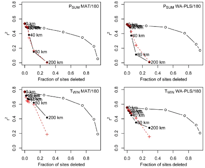
Therefore to check if spatial autocorrelation affects the western Patagonia training set we have 398
used the graphical method developed by Telford and Birks (2009). We compare the 399
performance of the WA-PLS and MAT as the training set size is reduced by deleting sites at 400
random, and by deleting sites geographically and environmentally close to the test site in 401
cross-validation (Fig. S3). In the case of autocorrelation, deleting geographically close sites 402
will preferentially delete the best analogues, and worsen the performance statistics more than 403
random deletion. If the observations are independent, deleting a given proportion of them 404
should have the same effect regardless of how they are selected (Telford and Birks, 2009). 405
Our results suggest that the r2 from deleting of geographical neighbourhood sites closely 406
follow the r2 from deleting the environmental neighbourhood sites indicating that PSUM and
407
TWIN are influenced by autocorrelation. The r2 scores strongly decrease after 40 km for PSUM
408
and after 80 km for TWIN and suggest that TWIN seems to be less affected by autocorrelation
409
than PSUM. This strong r2 decrease shows that if a large amount of sites are deleted from the
410
training set, the transfer functions are strongly affected by a lack of sample. This highlight the 411
limited size of our training set from a region characterized by a complex environmental and 412
vegetation gradient. In that case an enlarged dataset would be necessary to more rigorously 413
perform model cross-validation and to address more fully these problems of spatial 414
autocorrelation. However, another way to check the reliability of our models is to apply it to 415
fossil pollen data and to compare the signal with independent proxies. 416
417
4.3. Application of WA-PLS and the MAT to fossil pollen records
Here we applied the WA-PLS and the MAT to two oceanic pollen records, core MD07-3088 419
located at 46°S off Taitao Peninsula and core MD07-3104 located at 41°S in Reloncaví Fjord 420
(Figs. 1 and 6). Spanning the last deglaciation and the Holocene, pollen data from core 421
MD07-3088 illustrate the development of the North Patagonian Rainforest, which is 422
interrupted by an expansion of Magellanic Moorland during the Antarctic Cold Reversal 423
(ACR) (Montade et al., 2013). Located further north, the core MD07-3104 shows 424
compositional changes of temperate rainforest indicating warm and dry conditions during the 425
beginning of the Holocene and more climate variability from the mid-Holocene associated 426
with a cooling trend and with an increase of precipitation (Montade et al., 2012). Although 427
the climate reconstructions based on both models are consistent, the minor fluctuations 428
indicated by the MAT do not evidence significant climate changes. As previously mentioned, 429
this confirms that the MAT seems less appropriate than the WA-PLS to provide reliable 430
climate reconstructions according to our modern pollen-climate dataset. For that reason, the 431
climate reconstructions discussed below are based on the WA-PLS results. 432
Before 18 kyr, results obtained from core MD07-3088 at 46°S indicate lower values than 433
modern ones for PSUM (400-300 mm) and TWIN (ca. 3°C). However, before 18 kyr, these
434
results must be taken with caution given that during the late glacial, the pollen signal is 435
characterized by low pollen concentrations reflecting reduced or absent vegetation on the 436
adjacent land areas at a time, and the potential for non-analogue vegetation communities to be
437
present during the glacial and post-glacial transition, when glaciers were greatly expanded
438
compared to the present (Montade et al., 2013). Under these conditions an overrepresentation 439
of high producers of pollen such as Nothofagus trees was observed, which prevents local 440
vegetation reconstructions and which is likely to bias our climate reconstructions at that time. 441
From 18-17.5 kyr, a slight warming trend of 0.5°C is recorded, contemporaneous of the 442
beginning of the deglaciation evidenced by the δD variations of EPICA Dome C ice core (Fig. 443
6d). Such a trend occurs simultaneously with the development of vegetation following the 444
retreat of glaciers recorded in the region (Bennett et al., 2000; Haberle and Bennett, 2004). 445
Recorded from the same core, the beginning of the last deglaciation is also well evidenced by 446
the increase of summer sea surface temperature (SSTs, Fig. 6c) reconstructed from 447
planktonic foraminifera assemblages (Siani et al., 2013). The strongest change evidenced by 448
our climate reconstruction correspond to a rapid PSUM increase starting at 14.5 kyr (ACR) with
449
maximum values between 800 and 1000 mm. High PSUM values persist up to the end of the
450
Younger Dryas (YD) period (Fig. 6c). Simultaneously, we observe a progressive TWIN
451
increase of ca. 2°C while for the SSTs, values stop to increase during the ACR then decrease 452
of 1°C at 13 kyr before to reach maxima after the YD. This strong precipitation increase 453
characterised by very high values suggests an intensification of the SWW during the ACR and 454
the YD. Already recorded by previous studies from western Patagonia, this abrupt change was 455
interpreted as a northward shift of the SWW belt (García et al., 2012; Moreno et al., 2012; 456
Montade et al., 2015). Today, latitudes under the core of the SWW belt where rainfalls are 457
very high, the temperature seasonality is the lowest of western Patagonia and, because of 458
strong ocean influence, temperature values remain always positive at low elevation. 459
Consequently, after the last glacial conditions, such an intensification of SWW and 460
precipitation would have reduced the temperature seasonality inducing a milder summer and 461
winter temperature. This scenario might explain the observed TWIN increase by our
462
reconstruction. Based on this result, glacier advances evidenced in western Patagonia during 463
the ACR and the YD might be more related to hydrological changes than to a strong cooling 464
(Moreno et al., 2009; García et al., 2012; Glasser et al., 2012). However, additional 465
quantitative climate reconstructions are necessary to test this hypothesis. 466
After the YD, PSUM reconstructed from core MD07-3088 decrease progressively to reach
467
present-day values between 400 and 500 mm (Fig. 6a). TWIN values (ca. 6°C) are maxima
during the early Holocene, before they slightly decrease and fluctuate between 5 and 6°C, 469
close to modern values (Fig. 6c). This moderate change in comparison with the last 470
deglaciation are consistent with past vegetation dynamics recorded from the same latitude 471
showing that the North Patagonian Rainforest rapidly reaches its modern composition during 472
the early Holocene (Bennett et al., 2000). On the other hand, the core MD07-3104 indicates a 473
stronger climate variability during the Holocene. After reaching their maxima after the YD, 474
PSUM and TWIN decrease from 500 to 350 mm and from 11 to 8.5°C from the early to the
mid-475
Holocene (Figs. 6a and c). Then from 6 kyr, PSUM and TWIN fluctuate around 400 mm and 9°C
476
before a slight decrease during the late Holocene to reach values close to the modern 477
conditions. The climate variability reconstructed from core MD07-3104 is compared with a 478
pollen index calculated from Lago Condorito located at ca. 30 km from the oceanic core 479
(Moreno, 2004; Moreno et al., 2010). Based on the normalized ratio between Eucryphia-480
Caldcluvia and Podocarpus, positive values of this index reflect a warm-temperate,
481
seasonally dry climate with reduced SWW and negative values indicate cool-temperate and/or 482
wet conditions with enhanced SWW. While our reconstruction indicates that TWIN increase is
483
associated with PSUM increase, the pollen index indicates warm-temperate conditions under
484
low precipitation (Fig. 6). This difference might be related to a different sensitivity of 485
seasonality between the pollen index and our reconstructed TWIN. On the other hand,
486
comparison of PSUM curve and the index reveals the same trend. Although a short time lag is
487
observed, which is certainly related to a problem of marine age reservoir from the oceanic 488
core (Montade et al., 2012), our PSUM reconstruction supports the known dynamic of
489
precipitation and SWW changes in the region. Southward at 46°S, such changes are not 490
recorded by our climate reconstruction and by vegetation changes (Montade et al., 2013). 491
Today the northern Patagonia at 41°S is characterized by a seasonally dry climate directly 492
connected with a strong seasonality of SWW intensity. In comparison, the location of core 493
MD07-3088 closer to the position of the core of SWW already since the early Holocene, 494
under the persistent influence of the SWW, rainfalls are strong all over the year. 495
Consequently, this might explain why hydrological changes related to SWW changes would 496
have more impacted the northern Patagonia during the Holocene. 497
498
Conclusions
499
To conclude, although based on different depositional environments (soil, lake and ocean), 500
our modern pollen dataset (183 samples) from western Patagonia reflects the main vegetation 501
types distributed along the latitudinal and the altitudinal gradient. Investigating the modern 502
pollen-vegetation-climate relationships, we further demonstrate that the major vegetation 503
distribution reflected by pollen assemblages is mainly controlled by two parameters: PSUM and
504
TWIN. Characterized by a southward TWIN decrease and a southward PSUM increase, these two
505
parameters represent the main climatic limiting factor in western Patagonia controlling the 506
latitudinal distribution of the vegetation. Based on the modern pollen dataset, we then 507
analysed and compared the performance of two standard methods: the MAT and the WA-508
PLS. They adequately model taxa and their environments; however our results also reveal that 509
the WA-PLS is more suitable than the MAT which suffers of a lack of modern pollen samples 510
to perform reliable climate reconstructions. Using two oceanic cores from northern Patagonia 511
at 41°S and 46°S we finally proceeded to reconstructions of PSUM and TWIN values during the
512
late Glacial and the Holocene. The most important climate change occurred during ACR and 513
YD where PSUM reach the double amount of modern values related to an enhanced SWW.
514
Although our results show several methodological limitations (mainly by using oceanic and 515
terrestrial samples together), our climate reconstructions, consistent with the regional climate 516
changes, illustrate the potential to develop quantitative methods in western Patagonia. 517
Representing one of the parts of South America with the most pollen records, additional 518
quantitative climate reconstructions have to be performed to improve our understanding of 519
climate dynamic at a regional scale. Furthermore, the modern pollen dataset still needs to be 520
enlarged, to reduce uncertainties of climate reconstructions. 521
522
Acknowledgements
523
V.M. benefited from a postdoctoral position funded by Ecole Pratique des Hautes Etudes at 524
Institut des Sciences de l'Evolution de Montpellier (ISEM) and Deutsche 525
Forschungsgemeinschaft at Department of Palynology and Climate Dynamics from the 526
University of Goettingen. We thank Vera Markgraf for sharing pollen data and for helpful 527
comments on the first version of the manuscript. We also thank Elisabeth Michel and 528
Giuseppe Siani for sharing data concerning the oceanic core MD07-3088. Finally we are 529
particularly grateful from the very constructive comments from two anonymous referees 530
greatly improving this manuscript. This is an ISEM contribution n°XX. 531
532
References
533
Anderson RF, Ali S, Bradtmiller LI, Nielsen SHH, Fleisher MQ, Anderson BE, Burckle LH. 534
2009. Wind-Driven Upwelling in the Southern Ocean and the Deglacial Rise in 535
Atmospheric CO2. Science 323: 1443–1448.
536
Bennett KD, Haberle SG, Lumley SH. 2000. The Last Glacial-Holocene Transition in 537
Southern Chile. Science 290: 325–328. 538
ter Braak CJF, Juggins S. 1993. Weighted averaging partial least squares regression (WA-539
PLS): an improved method for reconstructing environmental variables from species 540
assemblages. Hydrobiologia 269–270: 485–502. 541
Brewer S, Guiot J, Barboni D. 2013. POLLEN METHODS AND STUDIES | Use of Pollen as 542
Climate Proxies. In Encyclopedia of Quaternary Science (Second Edition), Elias SA, 543
Mock CJ (eds). Elsevier: Amsterdam; 805–815. 544
Cao X, Herzschuh U, Telford RJ, Ni J. 2014. A modern pollen–climate dataset from China 545
and Mongolia: Assessing its potential for climate reconstruction. Review of 546
Palaeobotany and Palynology 211: 87–96.
547
Flantua SGA, Hooghiemstra H, Grimm EC, Behling H, Bush MB, González-Arango C, 548
Gosling WD, Ledru M-P, Lozano-García S, Maldonado A, Prieto AR, Rull V, Van 549
Boxel JH. 2015. Updated site compilation of the Latin American Pollen Database. 550
Review of Palaeobotany and Palynology 223: 104–115.
551
Francois J-P. 2014. Postglacial paleoenvironmental history of the Southern Patagonian 552
Fjords at 53°S. PhD thesis. Universität zu Köln.
553
Fréchette B, de Vernal A, Guiot J, Wolfe AP, Miller GH, Fredskild B, Kerwin MW, Richard 554
PJH. 2008. Methodological basis for quantitative reconstruction of air temperature and 555
sunshine from pollen assemblages in Arctic Canada and Greenland. Quaternary 556
Science Reviews 27: 1197–1216.
557
Gajardo R. 1994. La vegetación natural de Chile : clasificación y distribución geográfica. 558
Santiago. 559
García JL, Kaplan MR, Hall BL, Schaefer JM, Vega RM, Schwartz R, Finkel R. 2012. 560
Glacier expansion in southern Patagonia throughout the Antarctic cold reversal. 561
Geology 40: 859–862.
562
Garreaud R, Lopez P, Minvielle M, Rojas M. 2013. Large-Scale Control on the Patagonian 563
Climate. Journal of Climate 26: 215–230. 564
Garreaud RD, Vuille M, Compagnucci R, Marengo J. 2009. Present-day South American 565
climate. Palaeogeography, Palaeoclimatology, Palaeoecology 281: 180–195. 566
Glasser NF, Harrison S, Schnabel C, Fabel D, Jansson KN. 2012. Younger Dryas and early 567
Holocene age glacier advances in Patagonia. Quaternary Science Reviews 58: 7–17. 568
Grieser J, Giommes R, Bernardi M. 2006. New_LocClim - the Local Climate Estimator of 569
FAO. Geophysical Research Abstracts 8: 08305. 570
Guiot J. 1990. Methodology of the last climatic cycle reconstruction in France from pollen 571
data. Palaeogeography, Palaeoclimatology, Palaeoecology 80: 49–69. 572
Guiot J, de Vernal A. 2007. Chapter Thirteen Transfer Functions: Methods for Quantitative 573
Paleoceanography Based on Microfossils. In Developments in Marine Geology, 574
Hillaire–Marcel C, de Vernal A. (eds). Elsevier: Amsterdam; 523–563. 575
Haberle SG, Bennett KD. 2001. Modern pollen rain and lake mud-water interface 576
geochemistry along environmental gradients in southern Chile. Review of 577
Palaeobotany and Palynology 117: 93–107.
578
Haberle SG, Bennett KD. 2004. Postglacial formation and dynamics of North Patagonian 579
Rainforest in the Chonos Archipelago, Southern Chile. Quaternary Science Reviews 580
23: 2433–2452.
581
Harrison SP, Bartlein PJ, Prentice IC. 2016. What have we learnt from palaeoclimate 582
simulations? Journal of Quaternary Science 31: 363–385. 583
Heusser CJ. 2003. Ice age Southern Andes - A chronicle of paleoecological events. Elsevier: 584
Amsterdam. 585
Hijmans RJ, Cameron SE, Parra JL, Jones PG, Jarvis A. 2005. Very high resolution 586
interpolated climate surfaces for global land areas. International Journal of 587
Climatology 25: 1965–1978.
588
Juggins PS. 2015. rioja: Analysis of Quaternary Science Data. http://eprints.ncl.ac.uk. 589
Kilian R, Lamy F. 2012. A review of Glacial and Holocene paleoclimate records from 590
southernmost Patagonia (49–55°S). Quaternary Science Reviews 53: 1–23. 591
Lemieux-Dudon B, Blayo E, Petit J-R, Waelbroeck C, Svensson A, Ritz C, Barnola J-M, 592
Narcisi BM, Parrenin F. 2010. Consistent dating for Antarctic and Greenland ice 593
cores. Quaternary Science Reviews 29: 8–20. 594
Luebert F, Pliscoff P. 2004. Classification de pisios de vegetatacion y anlysis de 595
representatividad ecologica de areas propuesta para la proteccion en la ecoregion
596
valdivia. Santiago.
597
Mancini MV, de Porras ME, Bamonte FP. 2012. Southernmost South America Steppes: 598
vegetation and its modern pollen-assemblages representation. In Steppe Ecosystem 599
Dynamics, Land Use and Conservation, Germano D (ed). Nova Science Publishers:
600
New York; 141–156. 601
Markgraf V, Webb RS, Anderson KH, Anderson L. 2002. Modern pollen/climate calibration 602
for southern South America. Palaeogeography, Palaeoclimatology, Palaeoecology 603
181: 375–397.
604
Mauri A, Davis BAS, Collins PM, Kaplan JO. 2015. The climate of Europe during the 605
Holocene: a gridded pollen-based reconstruction and its multi-proxy evaluation. 606
Quaternary Science Reviews 112: 109–127.
607
Montade V, Combourieu-Nebout N, Chapron E, Mulsow S, Abarzúa AM, Debret M, Foucher 608
A, Desmet M, Winiarski T, Kissel C. 2012. Regional vegetation and climate changes 609
during the last 13 kyr from a marine pollen record in Seno Reloncaví, southern Chile. 610
Review of Palaeobotany and Palynology 181: 11–21.
611
Montade V, Combourieu-Nebout N, Kissel C, Haberle SG, Siani G, Michel E. 2013. 612
Vegetation and climate changes during the last 22,000 yr from a marine core near 613
Taitao Peninsula, southern Chile. Palaeogeography, Palaeoclimatology,
614
Palaeoecology 369: 335–348.
Montade V, Combourieu-Nebout N, Kissel C, Mulsow S. 2011. Pollen distribution in marine 616
surface sediments from Chilean Patagonia. Marine Geology 282: 161–168. 617
Montade V, Kageyama M, Combourieu-Nebout N, Ledru M-P, Michel E, Siani G, Kissel C. 618
2015. Teleconnection between the Intertropical Convergence Zone and southern 619
westerly winds throughout the last deglaciation. Geology 43: 735–738. 620
Moreno PI. 2004. Millennial-scale climate variability in northwest Patagonia over the last 15 621
000 yr. Journal of Quaternary Science 19: 35–47. 622
Moreno PI, Francois JP, Moy CM, Villa-Martínez R. 2010. Covariability of the Southern 623
Westerlies and atmospheric CO2 during the Holocene. Geology 38: 727–730.
624
Moreno PI, Kaplan MR, Francois JP, Villa-Martinez R, Moy CM, Stern CR, Kubik PW. 625
2009. Renewed glacial activity during the Antarctic cold reversal and persistence of 626
cold conditions until 11.5 ka in southwestern Patagonia. Geology 37: 375–378. 627
Moreno PI, Vilanova I, Villa-Martínez R, Garreaud RD, Rojas M, De Pol-Holz R. 2014. 628
Southern Annular Mode-like changes in southwestern Patagonia at centennial 629
timescales over the last three millennia. Nature Communications 5: 4375. 630
Moreno PI, Villa-Martínez R, Cárdenas ML, Sagredo EA. 2012. Deglacial changes of the 631
southern margin of the southern westerly winds revealed by terrestrial records from 632
SW Patagonia (52°S). Quaternary Science Reviews 41: 1–21. 633
Ortega-Rosas CI, Peñalba MC, Guiot J. 2016. The Lateglacial interstadial at the southeastern 634
limit of the Sonoran Desert, Mexico: vegetation and climate reconstruction based on 635
pollen sequences from Ciénega San Marcial and comparison with the subrecent 636
record. Boreas 45: 773–789. 637
Paez MM, Schäbitz F, Stutz S. 2001. Modern pollen–vegetation and isopoll maps in southern 638
Argentina. Journal of Biogeography 28: 997–1021. 639
Peyron O, Goring S, Dormoy I, Kotthoff U, Pross J, de Beaulieu J-L, Drescher-Schneider R, 640
Vannière B, Magny M. 2011. Holocene seasonality changes in the central 641
Mediterranean region reconstructed from the pollen sequences of Lake Accesa (Italy) 642
and Tenaghi Philippon (Greece). The Holocene 21: 131–146. 643
Prentice IC. 1980. Multidimensional scaling as a research tool in quaternary palynology: A 644
review of theory and methods. Review of Palaeobotany and Palynology 31: 71–104. 645
Schäbitz F, Wille M, Francois J-P, Haberzettl T, Quintana F, Mayr C, Lücke A, Ohlendorf C, 646
Mancini V, Paez MM, Prieto AR, Zolitschka B. 2013. Reconstruction of 647
palaeoprecipitation based on pollen transfer functions – the record of the last 16 ka 648
from Laguna Potrok Aike, southern Patagonia. Quaternary Science Reviews 71: 175– 649
190. 650
Schmithüsen J. 1956. Die räumliche Ordnung der chilenischen Vegetation. Bonner 651
Geographische Abhandlungen 17: 1–86.
652
Siani G, Michel E, De Pol-Holz R, DeVries T, Lamy F, Carel M, Isguder G, Dewilde F, 653
Lourantou A. 2013. Carbon isotope records reveal precise timing of enhanced 654
Southern Ocean upwelling during the last deglaciation. Nature Communications 4. 655
Telford RJ. 2015. palaeoSig: Significance Tests for Palaeoenvironmental Reconstructions. 656
Telford RJ, Birks HJB. 2005. The secret assumption of transfer functions: problems with 657
spatial autocorrelation in evaluating model performance. Quaternary Science Reviews 658
24: 2173–2179.
659
Telford RJ, Birks HJB. 2009. Evaluation of transfer functions in spatially structured 660
environments. Quaternary Science Reviews 28: 1309–1316. 661
Thompson RS, Anderson KH, Bartlein PJ. 2008. Quantitative estimation of bioclimatic 662
parameters from presence/absence vegetation data in North America by the modern 663
analog technique. Quaternary Science Reviews 27: 1234–1254. 664
Tian F, Herzschuh U, Telford RJ, Mischke S, Van der Meeren T, Krengel M, Richardson J. 665
2014. A modern pollen–climate calibration set from central‐western Mongolia and its 666
application to a late glacial–Holocene record. Journal of Biogeography 41: 1909– 667
1922. 668
Toggweiler JR, Russell JL, Carson SR. 2006. Midlatitude westerlies, atmospheric CO2, and
669
climate change during the ice ages. Paleoceanography 21: 1–15. 670
Tonello MS, Mancini MV, Seppä H. 2009. Quantitative reconstruction of Holocene 671
precipitation changes in southern Patagonia. Quaternary Research 72: 410–420. 672
Tonello MS, Prieto AR. 2008. Modern vegetation-pollen-climate relationships for the Pampa 673
grasslands of Argentina. Journal of Biogeography 35: 926–938. 674
Villa-Martínez R, Moreno PI, Valenzuela MA. 2012. Deglacial and postglacial vegetation 675
changes on the eastern slopes of the central Patagonian Andes (47°S). Quaternary 676
Science Reviews 32: 86–99.
677 678 679
Figure caption
680
681
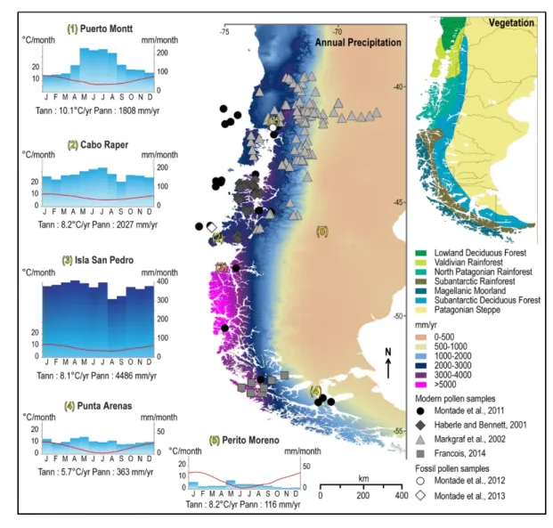
Figure 1. Climate and vegetation maps from Patagonia with location of modern samples and
682
fossil pollen records used in this study. Precipitation data were obtained from WorldClim 683
database (Hijmans et al., 2005), climatographs were performed using data from 684
meteorological stations (New_LocClim_1.10 software; Grieser et al., 2006) and vegetation 685
distribution is adapted from Schimithüsen (1956). 686
688
Figure 2. Pollen diagram of the 183 modern pollen samples from western Patagonia showing
689
the main pollen taxa. Ordination of modern pollen samples with pollen zones have been made 690
using a cluster analysis based on chord distance. According to the pollen assemblages of each 691
zone, six vegetation groups were identified: Grassland (G), Subantarctic Deciduous Forest 692
(SDF), Valdivian Rainforest (VR), North Patagonian/Valdivian Rainforest (NPR/VR), North 693
Patagonian/Subantarctic Rainforest (NPR/SR), Subantarctic Rainforest/Magellanic Moorland 694
(SR/MM). 695
697
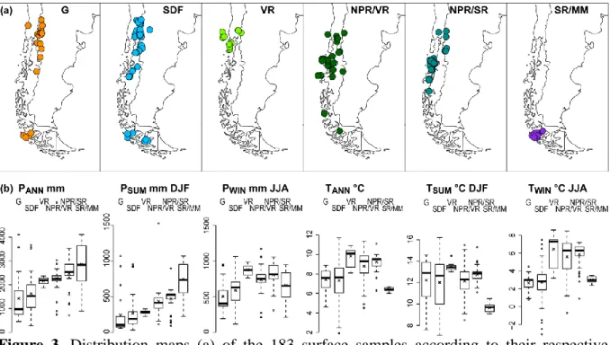
Figure 3. Distribution maps (a) of the 183 surface samples according to their respective
698
vegetation groups attributed from pollen assemblages: Grassland (G), Subantarctic Deciduous 699
Forest (SDF), Valdivian Rainforest (VR), North Patagonian/Valdivian Rainforest (NPR/VR), 700
North Patagonian/Subantarctic Rainforest (NPR/SR), Subantarctic Rainforest/Magellanic 701
Moorland (SR/MM). Boxplots (b) represent the main climate parameters of present-day 702
climate as they relate to the different vegetation groups: PANN and TANN correspond
703
respectively to the annual precipitation and the mean annual temperature, PSUM and PWIN
704
correspond respectively to the precipitation sum of December-January-February and June-705
July-August, TSUM and TWIN correspond to mean temperature of the same months as PSUM and
706
PWIN. The cross on each boxplot indicates the mean value for each climate parameter.
707 708
709
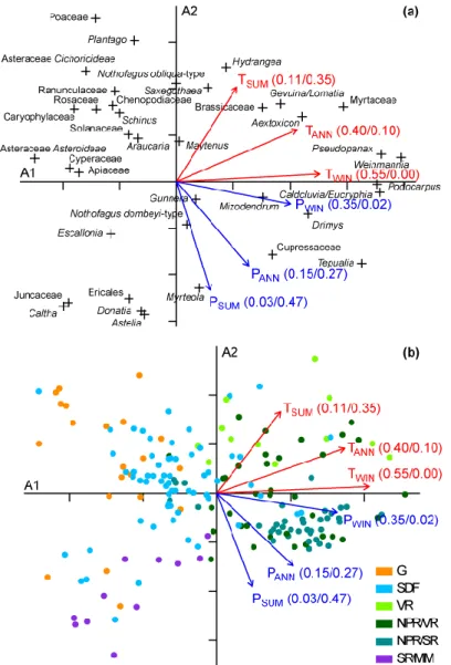
Figure 4. Bi-plot of the principal component analysis (PCA) with the 38 selected pollen taxa
710
(a) and the 183 selected modern pollen samples (b). Eigenvalues for the first and second axes 711
represent respectively 14% and 13% of the total variation. The arrows indicate the passive 712
climate parameter projected in the axes 1-2 bi-plot of the PCA with their respective r2: PANN
713
and TANN correspond respectively to the annual precipitation and the mean annual
714
temperature, PSUM and PWIN correspond respectively to the precipitation sum of
December-715
January-February and June-July-August, TSUM and TWIN correspond to mean temperature of
716
the same months as PSUM and PWIN. Grassland (G), Subantarctic Deciduous Forest (SDF),
717
Valdivian Rainforest (VR), North Patagonian/Valdivian Rainforest (NPR/VR), North 718
Patagonian/Subantarctic Rainforest (NPR/SR), Subantarctic Rainforest/Magellanic Moorland 719
(SR/MM). 720
721
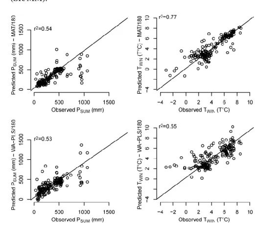
Figure 5. Comparison of predicted versus observed PSUM (precipitation sum of
December-722
January-February) and TWIN (mean temperature from June to August) performed on the 180
723
samples including oceanic and terrestrial pollen data from western Patagonia (excluding three 724
outliers) and using the Modern Analog Technique (MAT) and the Weighted Averaging Partial 725
Least Squares (WA-PLS). 726
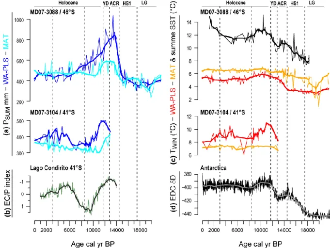
728
Figure 6. Climate reconstructions from core MD07-3088 and core MD07-3104 compared
729
with independent palaeoclimatic proxies. The PSUM (precipitation sum of
December-January-730
February) and TWIN (mean temperature from June to August) have been reconstructed using
731
the MAT (Modern Analog Technique) and the WA-PLS (Weighted Averaging Partial Least 732
Squares) with the pollen-climate training set of 180 samples. (a) PSUM from core MD07-3088
733
and MD07-3104; (b) EC/P (Eucryphia-Caldcluvia/Podocarpus) index from Lago Condorito 734
(Moreno, 2004); (c) SSTs (Summer Sea Surface Temperatures) from core MD07-3088 based 735
on planktonic foraminifera assemblages (Siani et al., 2013) with TWIN from core MD07-3088
736
and MD07-3104; (d) Ice-core δD based on the age scale of Lemieux-Dudon et al. (2010). The 737
original data were fit with a cubic smoothing spline (bold lines). YD, Younger Dryas; ACR, 738
Antarctic Cold Reversal; HS1, Heinrich Stadial 1; LGM, Last Glacial Maximum. 739
Table 1. Performance of the Weighted Averaging Partial Least Squares (WA-PLS) and the
741
Modern Analog Technique (MAT) based on leave-one-out cross-validation with 183 and 180 742
samples including oceanic and terrestrial pollen data from western Patagonia (PSUM,
743
precipitation sum of December-January-February; TWIN, mean temperature from June to
744
August). The table indicate the best selected component for each parameter and cross-745
validation test. 746
747
Model Component Variables Range r2 RMSEP RMSEP % of gradient Maximum Bias Average Bias MAT-183 - PSUM 31-1527 mm 0.49 180.8 12.1 1035 17.50 WA-PLS-183 2 PSUM 31-1527 mm 0.44 193.3 12.9 925 2.62 MAT-183 - TWIN -3.1-8.6 °C 0.77 1.1 20.3 2.1 2.08 WA-PLS-183 2 TWIN -3.1-8.6 °C 0.56 1.6 28.2 5.1 -0.05 MAT-180 - PSUM 31-1069 mm 0.54 162 15.6 446 17.31 WA-PLS-180 2 PSUM 31-1069 mm 0.53 164 15.8 266 -0.28 MAT-180 - TWIN -3.1-8.6 °C 0.77 1.1 20.4 2.1 -0.04 WA-PLS-180 2 TWIN -3.1-8.6 °C 0.55 1.6 28.5 5.1 -0.05 748 749