HAL Id: hal-02139030
https://hal.archives-ouvertes.fr/hal-02139030
Submitted on 28 Jan 2020
HAL is a multi-disciplinary open access
archive for the deposit and dissemination of
sci-entific research documents, whether they are
pub-lished or not. The documents may come from
teaching and research institutions in France or
abroad, or from public or private research centers.
L’archive ouverte pluridisciplinaire HAL, est
destinée au dépôt et à la diffusion de documents
scientifiques de niveau recherche, publiés ou non,
émanant des établissements d’enseignement et de
recherche français ou étrangers, des laboratoires
publics ou privés.
Implementation of an end-to-end model of the Gulf of
Lions ecosystem (NW Mediterranean Sea). II.
Investigating the effects of high trophic levels on
nutrients and plankton dynamics and associated
feedbacks
Frederic Diaz, Daniela Bănaru, Philippe Verley, Yunne-Jai Shin
To cite this version:
Frederic Diaz, Daniela Bănaru, Philippe Verley, Yunne-Jai Shin. Implementation of an end-to-end
model of the Gulf of Lions ecosystem (NW Mediterranean Sea). II. Investigating the effects of high
trophic levels on nutrients and plankton dynamics and associated feedbacks. Ecological Modelling,
Elsevier, 2019, 405, pp.51-68. �10.1016/j.ecolmodel.2019.05.004�. �hal-02139030�
UNCORRECTED
PROOF
Contents lists available at ScienceDirect
Ecological Modelling
journal homepage: www.elsevier.com
Implementation of an end-to-end model of the Gulf of Lions ecosystem (NW
Mediterranean Sea). II. Investigating the effects of high trophic levels on nutrients and
plankton dynamics and associated feedbacks
⋆
Frédéric Diaz
a, ⁎, Daniela Bănaru
a, ⁎, Philippe Verley
b, Yunne-Jai Shin
caAix Marseille University, Toulon University, CNRS, IRD, Mediterranean Institute of Oceanography (MIO) UM110, 13288, Marseille, France bIRD, UMR 123 AMAP, TA40 PS2, Boulevard de la Lironde, 34398 Montpellier Cedex 5, France
cIRD, UMR 248 MARBEC, Université de Montpellier, Bat. 24 – CC 093 Place Eugène Bataillon, 34095 Montpellier Cedex 5, France
A R T I C L E I N F O Keywords: End-to-end model Two-ways coupling Plankton Fisheries
Food web functioning
A B S T R A C T
The end-to-end OSMOSE-GoL model parameterized, calibrated and evaluated for the Gulf of Lions ecosystem (Northwestern Mediterranean Sea) has been used to investigate the effects of introducing two-ways coupling be-tween the dynamics of Low and High Trophic Level groups.
The use of a fully dynamic two-ways coupling between the models of Low and High Trophic Levels organisms provided some insights in the functioning of the food web in the Gulf of Lions. On the whole microphytoplank-ton and mesozooplankmicrophytoplank-ton were found to be preyed upon by High Trophic Levels planktivorous groups at rates lower than 10% and 25% of their respective natural mortality rates, but these relatively low rates involved some important alterations in the infra-seasonal and annual cycles of both High and Low Trophic Levels groups. They induced significant changes in biomass, fisheries landings and food web interactions by cascading effects. Spatial differential impacts of High Trophic Levels predation on plankton are less clear except in areas in which primary productivity is high. Higher predation rates on plankton groups were encountered within the area of the Rhone river’s influence and in areas associated to the presence of mesoscale eddies in the Northwestern part of the Gulf of Lions, especially. Generally, the pressure of the High Trophic Levels predation was the highest in areas of highest biomass whatever the plankton group considered.
The two-ways coupling between Low and High Trophic Levels models revealed both bottom-up and top-down controls in the ecosystem with effects on planktivorous species similar to those observed in the field. The use of the end-to-end model enabled to propose a set of potential mechanisms that may explain the observed decrease in small pelagic catches by the French Mediterranean artisanal fisheries over the last decade.
1. Introduction
Human activities interacting with climatic variability related to both natural and anthropogenic sources induce major changes in marine ecosystems (Halpern et al., 2008; Mora et al., 2013; Côté et al., 2016) that are difficult to understand and predict (Travers-Trolet et al., 2014; Piroddi et al., 2017). Fishing pressure together with the variability of physical forcing (e.g. winds, currents) may affect the structure and functioning of the entire food web due to the propagation of their
direct effects through top-down and bottom-up trophic cascades (Cury et al., 2003; Hunt and McKinnell, 2006). Moreover, drivers’ interaction may sometimes lead to synergistic effects, stronger than the isolated impact of each of these drivers (Travers-Trolet et al., 2014: Fu et al., 2018). As many marine systems show signs of degradation (Harpern et al., 2008; Bănaru et al., 2010; Piroddi et al., 2017), understanding how fisheries pressure, environmental conditions, and marine species inter-act is crucial (Côté et al., 2016), and has become a scientific priority to support key national and international conventions for better preserva
⋆ This manuscript is linked to the following research article: “Implementation of an end-to-end model of the Gulf of Lions ecosystem (NW Mediterranean Sea). I. Parameterization,
calibration and evaluation” by Bănaru et al. (2019), Ecological Modelling 401, 1–19, https://doi.org/10.1016/j.ecolmodel.2019.03.005.
⁎ Corresponding authors.
Email addresses: frederic.diaz@univ-amu.fr (F. Diaz); daniela.banaru@univ-amu.fr (D. Bănaru) https://doi.org/10.1016/j.ecolmodel.2019.05.004
Received 21 December 2018; Received in revised form 6 May 2019; Accepted 8 May 2019 Available online xxx
UNCORRECTED
PROOF
F. Diaz et al. Ecological Modelling xxx (xxxx) xxx-xxx
Fig. 1. Temporal dynamics of microplankton and mesozooplankton biomasses during the last eight years of simulation. The solid line represents total biomass summed over the whole
modeled domain. The vertical line delimits two periods with different coupling techniques between the Eco3M-S LTL model and the OSMOSE-GoL HTL model: one-way forcing mode from years 36 to 39 and two-ways coupling mode from years 40 to 43.
Table 1
Plankton biomass (in tons) preyed upon by HTL species. For years 36–39 (one-way forcing mode), the mean (± standard deviation) prey biomass annually eaten is reported. For years 40–43 (two-ways coupling mode), the annual plankton biomass preyed upon by HTL species is given. The three main size classes of predators (by decreasing order of ingested prey biomass) are indicated in abbreviations. K: northern krill, S<3: European sprat <3 cm, A<3: European anchovy <3 cm, A3-8: European anchovy (3–8 cm), A>8: European anchovy
>8 cm, P<3: European pilchard <3 cm, P3-12.5: European pilchard (3–12.5 cm), P>12.5: European pilchard >12.5 cm. NANOPHY = nanophytoplankton, MICROPHY =
microphytoplank-ton, NANOZOO = nanozooplankmicrophytoplank-ton, MICROZOO = microzooplankmicrophytoplank-ton, MESOZOO = mesozooplankton.
Years [36-39] 40 41 42 43 (2001) (2002) (2003) (2004) NANOPHY 1.47 ± 0.04 2.10 2.13 1.87 1.98 A<3,S<3,K A<3,S<3,K MICROPHY 24636 ± 180 26832 19357 19275 16653 P3-12.5,P>12.5,K P3-12.5,P>12.5,K P>12.5,P3-12.5,K K,P3-12.5,P>12.5 K,A3-8,P3-12.5 NANOZOO 0.133 ± 0.004 0.139 0.055 0.046 0.032 S<3,A<3,K S<3,A<3,K A<3,S<3,K S<3,K,A<3 A<3,S<3,K MICROZOO 29238 ± 1514 28127 24444 22672 20033 P3-12.5,P>12.5,A>8 P3-12.5,P>12.5,A>8 P>12.5,P3-12.5,A>8 P3-12.5,P>12.5,A3-8 A3-8,P3-12.5,P>12.5 MESOZOO 4714 ± 9 4254 4836 4682 5572 A>8,K,P3-12.5 A>8,P>12.5,P3-12.5 P<3,A>8,P>12.5 P<3,K,P>12.5
UNCORRECTED
PROOF
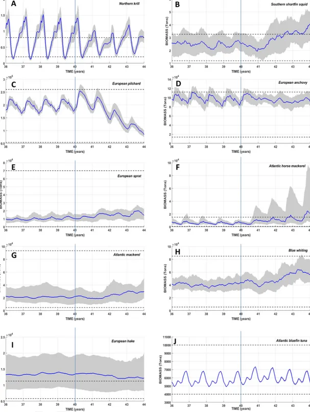
Fig. 2. Temporal evolutions of the simulated total biomass of the 10 HTL species during the last eight years of simulation over the whole modeled domain. The vertical line delimits the
temporal period of coupling technique between the Eco3M-S LTL model and the OSMOSE HTL model: coupled run in the one-way forcing mode from years 36 to 39 and in the two-ways coupling mode from years 40 to 43. The solid line shows the median value computed from the 50 simulation replicates. The lower and upper limits of the grey envelope delineate the 0.25 and 0.75 (respectively) percentiles computed from the 50 replicates. The two horizontal dotted black lines represent the range of observed biomass (Bănaru et al., 2019).
tion of natural ecosystems and sustainable use of biodiversity resources (e.g. European Marine Strategy Framework Directive; Convention on Biological Diversity, Inter-governmental Platform on Biodiversity and Ecosystem Services).
The semi-enclosed Mediterranean Sea has been considered as a hotspot for marine biodiversity (e.g. Bianchi and Morri, 2000; Coll et al., 2010) but it is also a “hotspot” for climate change (e.g. Giorgi,
2006; The MerMex Group et al., 2011). In parallel, the Mediterranean Sea, owing to its location between Africa, Europe and Asia, is under siege from many anthropogenic alterations such as the overexploitation of resources, habitat loss and various forms of pollution due to the rapid expansion of the demography all along its coasts (e.g. Coll et al., 2010, 2012; Lötze et al., 2011).
UNCORRECTED
PROOF
F. Diaz et al. Ecological Modelling xxx (xxxx) xxx-xxx
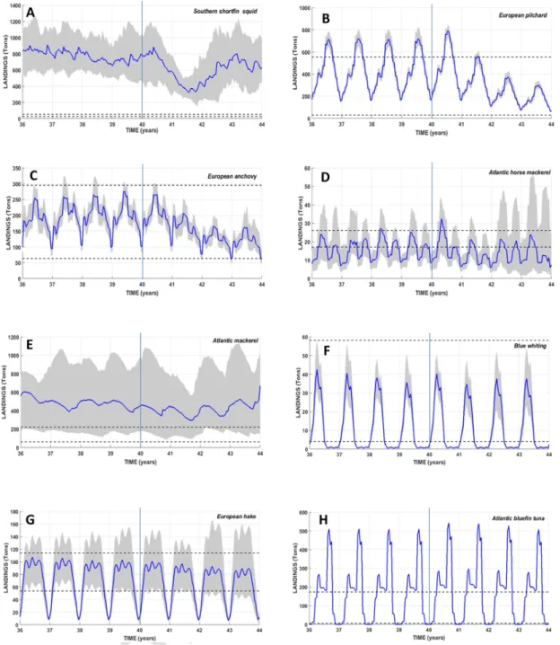
Fig. 3. Temporal evolutions of the simulated total landings of the 10 HTL species during the last eight years of simulation over the whole modeled domain. The vertical line delimits
the temporal period of the coupling technique between the Eco3M-S LTL model and the OSMOSE-GoL HTL model: coupled run in the one-way forcing mode from years 36 to 39 and in the two-ways coupling mode from years 40 to 43. The solid line shows the median value computed from the 50 simulation replicates. The lower and upper limits of the grey envelope delineate the 0.25 and 0.75 percentiles computed from the 50 simulation replicates. The two horizontal dotted black lines represent the range of observed landings (Bănaru et al., 2019).
In the Northwestern Mediterranean Sea, the Gulf of Lions (GoL) is characterized by a wide and shallow shelf. This area is one of the most productive zones of the Mediterranean Sea (e.g. Bosc et al., 2004) owing to heavy year-round nutrient inputs, mainly from the Rhone River (Lefèvre et al., 1997). It is thus an important feeding area for many resident and migratory High Trophic Level (HTL) species. As a result, 20% of the French fishing fleet operates in the GoL and 90% of the French Mediterranean landings take place in this area (Demaneche et al., 2009). Many fish species of commercial interest have been intensively exploited on the GoL continental shelf over the past decades by French and Spanish fleets using multi-specific arti-sanal gears (Farrugio et al., 1993; Sacchi, 2008). In this area, a study based on the ECOPATH mass-balance model suggested that some fish
species may be overfished with
respect to the amount of biomass necessary for the functioning of the food web (Bănaru et al., 2013). Forage species, such as European pilchard and European anchovy, representing usually more than 50% of the total catches in this area, are one of the most important prey groups, being a major trophic link between plankton and top preda-tors as some fish species, seabirds and mammals (Bănaru et al., 2013). However, over the last ten years, and despite the decrease in fishing pressure, the mean size and body condition of European pilchard and European anchovy have declined (Van Beveren et al., 2014; Saraux et al., 2018). Recent studies on their diet (Le Bourg et al., 2015) showed that they probably consume smaller prey than in the past, and that they maybe in competition with the European sprat, a non-commercial planktivorous fish which has strongly increased in biomass during re-cent years in this area. Some interesting questions arise from these ob
UNCORRECTED
PROOF
Table 2Values of the maximum HTL-induced mortality rates ( ), LTL mortality rates (mp) and
ra-tio of two parameters on plankton four groups. NANOPHY = nanophytoplankton, MICRO-PHY = microphytoplankton, NANOZOO = nanozooplankton, MICROZOO = microzoo-plankton, MESOZOO = mesozooplankton (see Banaru et al., 2019 for the definitions of ap
and Δt). mp Ratio (d−1) (d−1) NANOPHY 0.0394 0.000 – MICROPHY 0.0148 0.075 0.197 NANOZOO 0.0207 0.043 0.481 MICROZOO 0.0105 0.070 0.150 MESOZOO 0.0099 0.033 0.300
servations, such as why there has been a higher rate of consumption of smaller prey by planktivorous fishes over the past few years in this area? Have these small planktonic prey species been more abundant in recent years? And if so, is environmental forcing (winds, hydrodynam-ics) and its variability at different frequencies responsible for this alter-ation of the plankton community? In this context, the trophic and espe
cially size-based trophic interactions within the food web and the im-pact of the environmental conditions on these interactions are of crucial importance in order to understand the functioning and recent evolution of the GoL ecosystem.
Models that integrate the representation of the whole ecosystem from the dynamics of the physical environment to that of the highest trophic levels, the so-called end-to-end (E2E) models (see Rose, 2012 for an accurate definition), are useful tools to address the aforementioned ecological questions.
In the present study, the E2E model chosen to explore these ques-tions is the individual- and size-based model OSMOSE (Shin and Cury, 2004) with a configuration dedicated to the GoL, named OSMOSE-GoL, that has been recently parameterized, calibrated and confronted to ob-servations (see details in the companion paper Bănaru et al., 2019). One of the strengths of this configuration is to account for a fully dy-namic two-ways coupling between the models of Low Trophic Level (LTL) organisms (usually biogeochemical models) and HTL organisms. In this configuration of coupling, outputs of plankton groups provided by the LTL model serve as prey fields for the HTL organisms, which re-turn an additional predation mortality in the plankton groups. The im
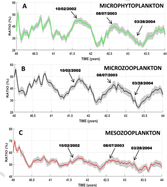
Fig. 4. Temporal evolutions of the HTL predation pressure (see Section 3.4. for a detailed definition) on mesozoo- and microplankton groups over the whole modeled domain under the
two-ways coupling mode. The solid line shows the median levels computed from the 50 simulation replicates. The lower and upper limits of the grey envelope delineate the 0.25 and 0.75 percentiles computed from the 50 simulation replicates. Black arrows and associated dates indicate the dates of spatial distributions showed on Figs. 5–8.
UNCORRECTED
PROOF
F. Diaz et al. Ecological Modelling xxx (xxxx) xxx-xxx
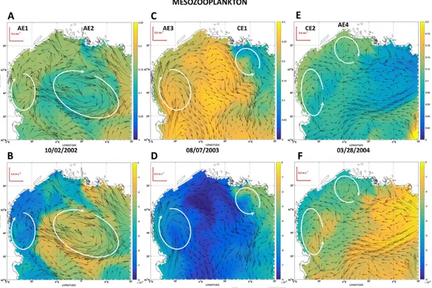
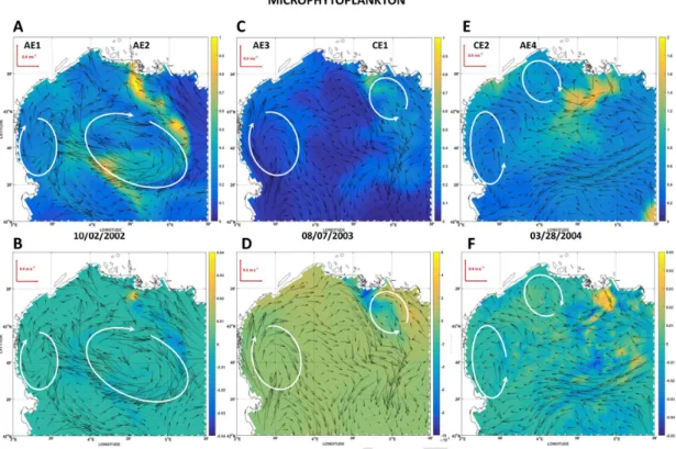
Fig. 5. Surface fields of mesozooplankton modeled biomass (mmol m−3) at three selected dates along the simulation. For a given date, upper panels show plankton biomass resulting from
the OSMOSE-GoL model (two-ways coupling mode between HTL and LTL models). The lower panels show patterns of differences (OSMOSE-GoL minus LTL model) in biomass (mmol m−3).
Vectors represent the surface field of currents at the corresponding date. The locations of hydrodynamic structures of interest as mesoscale cyclonic (CE) and anticyclonic (AE) eddies are indicated by the white ellipses.
Fig. 6. Same caption as Fig. 5 for microzooplankton biomass (in mmol m−3).
plementation of E2E models has rarely been undertaken in a dynamic two-ways coupling between LTL and HTL models but rather in a one-way forcing mode with outputs from biogeochemical models being used as forage fields for HTL organisms without any feedback on the
LTL biomass and distributions. As a result, the effects of the type of models' coupling (with or without feedbacks from HTL to LTL organ-isms) on ecosystem dynamics have only been documented for the ma
UNCORRECTED
PROOF
Fig. 7. Same caption as Fig. 5 for microphytoplankton biomass (in mmol m−3).
Fig. 8. Same caption as Fig. 5 for phosphate concentrations (in mmol m−3).
rine ecosystem of the Benguela Current (Travers-Trolet et al., 2009, 2014) to the best of our knowledge.
The aims of the present study are therefore the following. (i) To as-sess the impact of the two-ways coupling between the LTL and HTL sub-models on the outputs of the E2E model. This evaluation will be undertaken through the analysis of changes in the temporal dynamics of the biomass and landings of living resources, in predation pressure
on plankton groups and in the resulting trophic cascade effects. (ii) To evaluate the order of magnitude and potential impacts of the two-ways coupling and hydrodynamic processes (meso-scale eddies, region of freshwater influence by Rhone River) on the spatial distribution of plankton and nutrients. (iii) To propose hypotheses to enlighten the en-vironmental causes of the observed fluctuating stocks of certain fish species (e.g. European anchovy, European pilchard, and European
UNCORRECTED
PROOF
F. Diaz et al. Ecological Modelling xxx (xxxx) xxx-xxx
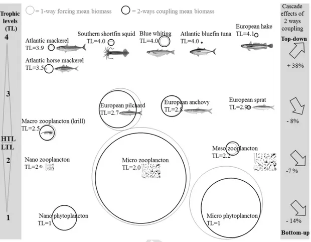
Fig. 9. Cascade effects on food web groups and species biomass and food web controls between the two-ways coupling mode vs. one-way forcing mode. Arrows indicate change in biomass
by trophic level. Circle size is proportional to their mean biomass. Grey circles indicate the mean biomass in the one-way forcing mode (years 36–39) and black circles indicate the mean biomass in the two-ways coupling mode (years 40–43).
Fig. A1. Temporal dynamics of nanophytoplankton biomasses during the last eight years of simulation. The solid line represents total biomass summed over the whole modeled domain.
The vertical line delimits two periods with different coupling techniques between the Eco3M-S LTL model and the OSMOSE-GoL HTL model: one-way forcing mode from years 36 to 39 and two-ways coupling mode from years 40 to 43.
UNCORRECTED
PROOF
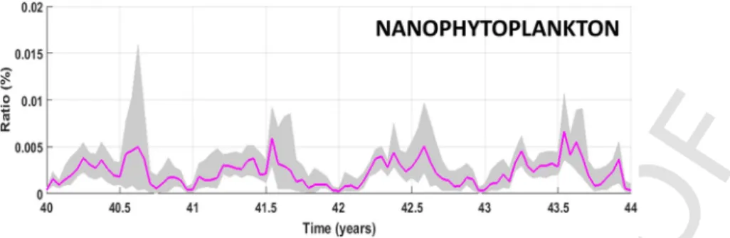
Fig. A3. Temporal evolutions of the HTL predation pressure (see Section 3.4. for a detailed definition) on nanophytoplankton groups over the whole modeled domain under the two-ways
coupling mode. The solid line shows the median levels computed from the 50 simulation replicates. The lower and upper limits of the grey envelope delineate the 0.25 and 0.75 percentiles computed from the 50 simulation replicates.
Fig. A4. Same caption as Fig. A3 for nanozooplankton.
sprat). The E2E model was run over a four-year period characterized by contrasted environmental conditions, involving a high interannual vari-ability of the biomass of certain plankton groups. The analysis of this run may enable to disentangle the respective roles of bottom-up and top-down processes on the seasonal and interannual dynamics of HTL organisms. This type of analysis is crucial to raise our capacity in mov-ing towards Ecosystem Based Management of the fisheries in the GoL marine area.
2. Methods
The OSMOSE-GoL model that has been previously described, para-metrised, calibrated and evaluated in the companion paper (Bănaru et al., 2019), is used in this study to achieve the aforementioned aims. This E2E model is composed of two sub-models. The first is the Eco3M-S/ Symphonie model (Campbell et al., 2013) that represents the dynam-ics of LTL organisms influenced by hydrodynamdynam-ics and meteorological processes. The second is the individual-based model OSMOSE (Shin and Cury, 2004; Grüss et al., 2015) that simulates the dynamics of HTL or-ganisms. The design of the numerical experiment is detailed in the com-panion paper (Bănaru et al., 2019), but its main points are reminded in the following for sake of clarity. The OSMOSE-GoL is firstly cali-brated using an optimization technique relying on an evolutionary al-gorithm and a likelihood-based objective function (Oliveros-Ramos and Shin, 2016). The calibrated model is then run in the one-way forcing configuration and feed in loop on the numerical fields of LTL biomass for year 2001, until a realistic equilibrium is reached in the levels of HTL outputs (Bănaru et al., 2019). This equilibrium is reached after a period of 35 years that is considered as a spin-up period. Following this spin-up period, the OSMOSE-GoL model is run first in the one-way mode during years 36 to 39 and then in the two-ways coupling mode by re-ceiving the numerical fields of LTL biomass from years 2001 to 2004 (corresponding to years referred to as 40 to 43 hereafter). A set of 50 simulations was launched to account for the stochasticity of the OS-MOSE model. The one-way forcing period (years 36 to 39) as well as the period of two-ways coupling mode (years 40 to 43) have been con
sidered for analysis in the following sections. Mean, median (and asso-ciated percentiles) values are used to synthetically present and analyze the outputs of the model.
3. Results
3.1. Temporal dynamics of plankton biomass
The annual cycles of microphytoplankton (Fig. 1A) show the high-est levels of biomass along winter period and at the onset of spring in the one-way forcing mode. The summer season is characterized by the lowest biomasses and weakest variations. Autumn is characterized by an increase in biomass that is of lower intensity than that of the spring. A more pronounced interannual variability of seasonal dynamics can be noted under the two-ways coupling mode. The intensity and duration of winter peak are very variable depending on the year. The sharp de-crease in biomass occurring later during spring is always present. Au-tumnal peak can be present on some years (e.g. 40, 42) while absent on the other ones. The microphytoplankton biomass yearly eaten (Table 1)
is on average ˜24.6 103tons (s.d. 180 tons) in the one-way forcing mode
which represents from 3 to 16% of the available stock. Over year 40,
the biomass eaten increases to nearly 27 103tons, that is 18% of the
available stock. The microphytoplankton biomass annually consumed
by predators significantly falls down to 19 103tons during the following
two years 41 and 42, and drastically decline again to 16.7 103tons
dur-ing year 43. Whatever the coupldur-ing mode, the main predators of micro-phytoplankton are the two largest classes (>3 cm) of European pilchard and northern krill. However, in year 43, the intermediate size class of European anchovy (3–8 cm) appears to be the second most important predator, at the expense of the largest European pilchard (>12.5 cm).
The annual cycle of microzooplankton biomass (Fig. 1B) in the one-way forcing mode shows sharp variations of biomass throughout the years while, in the two-ways coupling mode, the variability is less marked. In the one-way forcing mode, biomass is at its minimum at the
UNCORRECTED
PROOF
F. Diaz et al. Ecological Modelling xxx (xxxx) xxx-xxx
the year is characterized by a decreasing trend of biomass until the end of autumn, punctuated by large and rapid variations such as a recur-rent summer peak of biomass. The last three years of simulation in the two-ways coupling mode have the common point of showing a mini-mum biomass moved forward during autumn and a delayed peak occur-ring at the end of winter (years 41 and 42) or even duoccur-ring spoccur-ring (year 43). The amount of microzooplankton yearly eaten is slightly higher
than 29 103tons on average in the one-way forcing mode (Table 1)
and decreases gradually throughout the simulated years in the two-ways
coupling mode down to ca. 20 103tons (year 43), then representing
ca. 10% of the autumnal minimum. The largest size classes of European
pilchard (>3 cm) and European anchovy (>8 cm) are, on average, the main predators of microzooplankton in the two coupling modes. How-ever, it can be noted that there is a certain decrease in the predator size (e.g. European anchovy) since the intermediate size class appears to be one of the three main predators, at the expense of the largest size class from year 42.
As for microzooplankton, the annual cycle of the mesozooplankton biomass (Fig. 1C) in the one-way configuration strongly differs from those occurring in the two-ways mode. In the one-way configuration, minima levels of biomass are found during winter, followed by a sharp increase from spring to summer peaking at the end of summer. Then biomass quickly falls by ca. 40% before a slower decrease during au-tumn, then a sharper fall at the onset of the following winter. The sea-sonal cycles in the two-ways configuration are marked by a strong inter-annual variability. While the minimum biomass in winter increases over the years, the seasonal peaks of biomass are reached in spring, summer, autumn of years 42, 41, 43, respectively. The amount of mesozooplank-ton eaten yearly is 4714 mesozooplank-tons on average in the one-way configuration (Table 1), ranging between 5 and 15% of the available stock. In con-trast to the dynamics of predation on all other planktonic prey, there is no clear trend in the quantity of mesozooplankton eaten over the years in the two-ways configuration. It is worth noting that the amount of eaten biomass is the highest one (5572 tons) during year 43, in line with the sharp increase in available biomass during the second part of that year (Fig. 1C). The European anchovy (exclusively >8 cm) and Euro-pean pilchard (all size classes) are the main predators of mesozooplank-ton. The northern krill can occasionally be the second most important predator, as in years 42 and 43, and in the one-way configuration. It is interesting to note that, while the amount of eaten biomass increases by
ca. 20% from year 42 to 43, the ranking of the main predators does not
change.
The seasonal cycle of the nanophytoplankton biomass (Fig. A1) shows a minimum at the end of winter followed by an increase from spring to the end of autumn. The year-to-year variability of the bio-mass cycle is marked over the period of the two-ways coupling mode. The amount of nanophytoplankton consumed compared to the available stock (Fig. A1) remains extremely low (<0.004%) whatever the cou-pling mode considered (Table 1). However, this amount increases by ˜40% in the two-ways coupling mode. The smallest size classes of Euro-pean anchovy, EuroEuro-pean pilchard as well as northern krill are the main predators of nanophytoplankton whatever the linking mode considered. The annual cycles of nanozooplankton in the one-way forcing mode (Fig. A2) show an abrupt increase at the onset of winter followed by a sharp drop to very low levels along the rest of the year. Years 41–43 are characterized by a strong erosion of the winter peaks. The nanozoo-plankton biomass yearly eaten (Table 1) is very low (ca. 0.13 tons on average) in the one-way forcing mode and even lower when two-ways coupling is implemented, representing a tiny proportion of the plank-tonic food (<0.005%). As expected, the smallest sizes (<3 cm) of Euro-pean sprat and EuroEuro-pean anchovy as well as northern krill are the main predators of nanozooplankton.
3.2. Temporal dynamics of HTL species biomass
The seasonal dynamics of HTL species resulting from the one-way forcing mode have been already depicted in detail by Bănaru et al. (2019) and only the seasonal cycles produced under the two-ways cou-pling mode are hereafter described (years 40 to 43 in Fig. 2).
Most of the modeled biomass of HTL species shows interannual changes in median values within the ranges of biomass estimates from field observations, except that of European hake which is slightly over-estimated.
The median biomass of northern krill (Fig. 2A) shows wide varia-tions, with the highest and lowest values occurring in winter and the end of spring, respectively. Interannual variability of the seasonal cycle can be noted. For example, the autumnal plateau does not exist during year 42 and show a continuous increase up to a peak of biomass reached during the next winter. This year 43 winter maximum is ˜30% higher than those of previous years.
At the onset of the two-ways coupling, the biomass of southern
short-fin squid (Fig. 2B) decreases from ˜2.5 104tons down to ˜2 104tons. The
following two years show, on the contrary, a continuous and strong in-crease in biomass with only slight seasonal variations.
The temporal dynamics of European pilchard (Fig. 2C) show reg-ular seasonal variations, with maxima reached at the onset of spring and minima at the entrance of winter. The yearly range of extreme val-ues is wide, with variations of 30–40% of the biomass. During year 40,
the spring maximum of biomass reaches ˜2.6 105tons, while the
mini-mum is around 1.80 105tons. The following years then show a global
decrease in the biomass levels, with lower and lower spring maxima
(<1.25 105tons in year 43).
During year 40, the median biomass of European anchovy (Fig. 2D) shows a seasonal cycle characterized by highest biomass from mid-win-ter to the end of spring, and lowest biomass during autumn. This sea-sonal dynamic almost entirely disappears the following years, with spring peaks barely detectable (e.g. years 41 and 43).
The seasonal variations in the biomass of European sprat (Fig. 2E) are weak. However, the range of variations is more marked under the two-ways configuration. Highest biomass occurs at the end of spring while the lowest is found at the beginning of winter. The highest
me-dian biomass reaches ˜2 104tons during year-43, and is almost twice the
maximum of year 40.
The dynamic of Atlantic horse mackerel (Fig. 2F) has common points with that of European sprat. Seasonal variations in biomass are weak, but they perceptibly increase under the two-ways configuration. Fur-thermore, the biomass peaks regularly increase reaching up to ca. 2.5
104tons at the autumn end of year 43, that is 35% more than the
maxi-mum reached during year 40. In parallel, there is a larger spread of the percentiles range especially towards the high values of biomass.
A very weak seasonal signal can be observed in the simulated bio-mass of Atlantic mackerel (Fig. 2G). The amplitude of variations be-tween maxima from end of winter to mid-spring and minima from mid-summer to mid-autumn does not exceed ˜12%. However, year 41 is characterized by the absence of biomass peak at the end of winter. The last two years show a significant increase in biomass levels by >20% compared to previous years.
The biomass of blue whiting (Fig. 2H) does not show any clear
sea-sonal pattern. Median biomass fluctuates around 4 104tons during year
40 and the three last years are characterized by an increase in the
bio-mass up to 6.5 104tons.
The biomass of European hake (Fig. 2I) does not show any signifi-cant seasonal signals. The level of biomass remains almost constant (˜1.4
104tons) during years 40 and 41, but a slight decrease (˜10%) occurs
UNCORRECTED
PROOF
The median biomass of Atlantic bluefin tuna (Fig. 2J) shows a marked seasonal cycle. A minimum biomass during winter (˜5000-5500 tons) is followed by a rapid increase up to a first peak at the onset of spring (˜5600-6200 tons). Another minimum biomass oc-curs at the entrance of summer, and then the annual peak (˜7000 tons) occurs during every autumn. A slight increase in biomass (+10%) is noted, especially during the first three years under two-ways configura-tion.
3.3. Temporal dynamics of HTL species landings
The temporal dynamics of HTL species landings results from the in-put parameters of the model and particularly fishing mortality and sea-sonality that remain constant over the whole modeled period (Bănaru et al., 2019) and of the dynamics of the exploited stocks and the food web interactions.
As in the one-way configuration (Bănaru et al., 2019), the modeled landings of most of the HTL species (except southern shortfin squid and Atlantic mackerel) stand within the ranges of observed data (Fig. 3). Catches of northern krill and European sprat (results not shown) are not computed by the model as they are not landed by fishermen.
The temporal dynamics of HTL species with planktivorous-dominant diet, such as southern shortfin squid (Fig. 3A), European pilchard (Fig. 3B) and European anchovy (Fig. 3C) have in common to show signif-icant changes between year 40 and the following three years. For the latter two species, the seasonality of the landings remains similar, but a significant decline occurs over years 41–43. For the southern shortfin squid (Fig. 3A), both the seasonal cycle and the level of landings change radically. The landings are almost stable during the first part of year 40, and then sharply fall of more than 50% until the middle of year 41. The years 42 and 43 show an increase up to ca. 700 tons without a clear sea-sonal cycle.
The temporal dynamics of Atlantic horse mackerel (Fig. 3D) shows a seasonal cycle composed of two maxima (spring and autumn) and two minima (winter and summer). The spring maximum is considerably higher than that of autumn except in year 42. Year 40 shows the high-est spring peak, with landings exceeding 30 tons. In parallel, the winter minimum (˜8 tons) is generally lower than that of summer, except for year 42. The last two years are characterized by a larger spread of the percentiles range especially with regard to the high values of landings during spring.
Landings of Atlantic mackerel (Fig. 3E) increase during autumn and peak at the onset of winter. They then decline slowly down to minimum levels at the end of summer. The seasonal cycle is generally weakly marked. Year 43 shows an overall increase in landings by ˜15%.
The seasonality of landings of blue whiting (Fig. 3F) is almost un-changed in two-ways configuration. Landings are close to zero during autumn, and sharply increase during winter up to their maximum lev-els. This peak is transient and landings drastically fall in two phases. A small decline first occurs at the onset of summer, followed by a short stabilization, then landings quickly drop to zero during the second part of summer.
Maximum landings of European hake (Fig. 3G) oscillate from mid-winter to the end of summer between 90 and 100 tons during years 40 and 41 and between 80 and 90 tons during years 42 and 43. Autumn is characterized by a sharp decline down to a minimum of ˜10 tons, and the onset of winter shows a sharp increase up to the seasonal maximum. The pattern of annual dynamics of landings for Atlantic bluefin tuna (Fig. 3H) shows marked seasonal variations and a regular cycle during years 40 to 43. Modeled landings are close to zero from mid-autumn to the beginning of winter which corresponds to the period when bluefin tuna migrates out of this area. A first increase peaking at ˜280 tons fol
lows in spring. A second much higher peak (˜500 tons) then occurs dur-ing autumn.
3.4. Temporal dynamics of the HTL predation pressure on the plankton groups
The level of HTL pressure is defined as the ratio between the actual HTL-induced mortality rates and their potential maximum value (Table 2) for each group of planktonic prey.
The median levels of HTL predation pressure on the microphyto-plankton group (Fig. 4A) oscillate between 25% and 50%. The second part of the year is generally marked by the highest pressure with a peak during summer. The minimum pressure generally occurs during win-ter or even spring, as in year 43. There are, however, some significant differences in the annual cycle between years. The seasonal pattern of year 40 shows rather wide and rapid variations, with a minimum oc-curring at the beginning of winter, followed by an overall increase until reaching two successive peaks of around 47% in summer and autumn. The years 41–43 show (i) lesser variability, and (ii) a decreasing trend of predation characterized, for example, by lower and lower peaks and minima.
The HTL predation pressure on the microzooplankton group (Fig. 4B) oscillates between 25 and 55%. The seasonal pattern mirrors that of microphytoplankton: a predation minimum occurs at the end of win-ter and is followed by an overall increase from spring to mid-autumn. Year 40 differs from the last three years by wide variations and a marked winter peak. Interannual variability can be also noticed with a pressure minimum moved forward mid-winter (i.e. year 42) or delayed mid-spring (i.e. years 41, 43). Overall, predation pressure tends to de-crease over the simulated four years.
The levels of HTL predation pressure on the mesozooplankton group (Fig. 4C) are ca. 50% for most of the simulation period, except at the beginning of year 40 for which ratios exceed 60%. The seasonal pat-tern generally shows two periods of high pressure. The first one hap-pens in winter and lasts until the onset of spring (i.e. year 43), and the second one extends from mid-summer to the end of autumn. The spring period is then rather characterized by a minimum. From years 41 to 43, the winter maximum appears to be strongly reduced while the autumn maximum becomes dominant. As previously noted for the microplank-ton groups, there is globally a slow decrease in the predation pressure over the simulated period.
The pressure of predation on the nanoplankton groups (Figs. A3 & A4) remains very low (<0.005-0.006%) under the two-ways configura-tion. The highest pressures of predation generally happen from the on-set of the spring to that of autumn (e.g. year 43).
3.5. Spatial effects of two-ways coupling on plankton and nutrients
Three snapshots over the simulation period are hereafter shown to il-lustrate how the two-ways coupling can affect the spatial fields of plank-ton and even those of nutrients indirectly. Horizontal (Figs. 5–8) fields from February 2002, August 2003 and March 2004 are examined in details because these periods correspond to occurrences of high preda-tion pressure by HTL (Fig. 4) which can involve a direct consumppreda-tion of plankton prey but also some trophic cascading effects within the LTL. Only the distributions of prey (i.e. microphytoplankton, mesozooplank-ton and microzooplankmesozooplank-ton) for which the HTL predation pressure was the highest (predation ratio >20%, Fig. 4) over the simulation period are shown as well as those of phosphate contents, a nutrient potentially controlling the level of primary productivity in the GoL (e.g. Diaz et al., 2001).
To check the spatial effects of the two-ways coupling on plank-ton and nutrient, we compared numerical fields from the OSMOSE-GoL model (upper panels of Figs. 5–8) to those without considering any
UNCORRECTED
PROOF
F. Diaz et al. Ecological Modelling xxx (xxxx) xxx-xxx
coupling with OSMOSE model, i.e. only resulting from the LTL Eco3M-S/Symphonie model (Campbell et al., 2013). Easier comparisons are made by considering fields of differences (concentrations with HTL predation in two-ways configuration minus those without any HTL pre-dation) for plankton and phosphate (lower panels of Figs. 5–8).
The first snapshot to be analyzed happens during the beginning of autumn 2002, and two remarkable hydrodynamic structures under the form of anticyclonic eddies AE1 and AE2 (plots A and B of Figs. 5–8) are present at this period in the GoL. AE1 is of rather small size with an el-liptical shape (large semi-axis ca. 60 km, small semi-axis ca. 40 km), and is entirely located in the southwestern part of the OSMOSE-GoL domain while AE2 is much larger (large semi-axis ca. 140 km, small semi-axis
ca. 70 km) and only partly located in the OSMOSE-GoL domain. These
two eddies as well as the region of freshwater influence (ROFI) of the Rhone River (Diaz et al., 2008) mostly shape the distributions of plank-ton groups and to a lesser degree, that of phosphate. On the whole, the edges of the eddies show difference in biomass or concentrations com-pared to their center, or even, their surrounding water masses. Depend-ing on the plankton groups considered, these AE (AE2, especially) show at their edges either higher biomass in microphytoplankton, microzoo-plankton (Figs. 6A & 7A) or lower stocks in mesozoomicrozoo-plankton (Fig. 5A) than those around. The ROFI of the Rhone River is clearly identified
by the area of phosphate high concentrations (>0.15 mmol m−3on Fig.
8A). The ROFI is characterized by either high microphytoplankton and microzooplankton biomass on its western edge especially, or low meso-zooplankton biomass (upper panels and first column of Figs. 5A, 6A, 7A). Several intriguing features appear from the examination of the dif-ference maps (lower panels of Figs. 5–8). When the whole modeled do-main is considered, there is generally lower biomass in mesozooplank-ton and microphytoplankmesozooplank-ton (Fig. 5B & 7B) and slightly higher micro-zooplankton and phosphate stocks (Fig. 6B and 8B) in the two-ways cou-pling mode. The orders of magnitude of differences show strong vari-ations from one plankton group to another and for phosphate: up to a few percent of the available stock for microzooplankton and microphy-toplankton, but much lower than 1% for phosphate and mesozooplank-ton. Spatial gradients on the difference maps are marked for plankton especially in the vicinity of AE2 and the ROFI of the Rhone River. For example, implementing the two-ways coupling had a lower impact on mesozooplankton patterns both in the center and on the edges of AE2 than that modeled on the western part of the GoL shelf (Fig. 5B). By con-trast, the impact of considering two-ways coupling on microzooplank-ton and microphytoplankmicrozooplank-ton patterns was especially high on the edges of AE2 (Fig. 6B & 7B). Within the ROFI of the Rhone River, the ac-count for the two-ways coupling provokes less changes on the two zoo-plankton groups than those modeled at the edges of AE. The ROFI is also the only zone in this snapshot to show positive differences in mi-crophytoplankton biomass (Fig. 7B) indicating a stronger presence of this prey when the two-ways coupling is explicitly accounted for. Differ-ences in phosphate concentrations are hardly detectable at the edges of AE2. On the whole, the spatial structuration of nutrients and plankton near the small-sized AE1 does not show marked alterations whether the two-ways coupling is activated or not only except for microzooplankton. The second snapshot to be analyzed happens during the mid-sum-mer 2003 when two remarkable hydrodynamic structures (anticyclonic eddy AE3 and cyclonic eddy CE1, Fig. 5C) are present in the OS-MOSE-GoL domain. AE3 is of medium size with an elliptical shape (large semi-axis ca. 65 km, small semi-axis ca. 50 km) on the southwest-ern side of the GoL. CE1 is a smaller structure of almost circular shape (radius ca. 40 km). CE1 clearly interacts at the time of the snapshot with the ROFI of the Rhone River that can be finely located by the surface distribution of phosphate concentrations (Fig. 8C). The distributions of plankton groups and phosphate on the northeastern and southwest-ern sides were mainly constrained by CE1 and AE3 respectively. High
mesozooplankton biomass (˜0.25 mmol m−3, Fig. 5C) is modeled in the
central part of the GoL shelf, while a sharply decreasing biomass gradi-ent occurred in the northeastern part of the shelf owing to the presence of CE1. In the southwestern part of the GoL, mesozooplankton biomass was slightly lower at the edges of AE3 than in surrounding areas.
Surface structuration of microzooplankton biomass is almost the op-posite of that of mesozooplankton biomass. High microzooplankton bio-mass was modeled in the northeastern part of the GoL shelf and near the Rhone River mouth, and the flow of CE1 tended to advect these high biomass southwestwards (Fig. 6C). Similar spatial patterns could be ob-served for modeled phosphate concentrations (Fig. 8C). Depletion in modeled microphytoplankton was found in the central part of the shelf while the surrounding water masses near eddies showed higher biomass (Fig. 7C). The resulting flow of these two eddies involved an export in microphytoplankton from the coastal area to the offshore zone. In this second snapshot, the two-ways coupling generally provoked the high-est losses of plankton in areas of highhigh-est biomass whatever the group considered. For example, the northeastern area near CE1 and the Rhone River mouth showed the highest biomass of microphytoplankton and microzooplankton (Figs. 6C & 7C) and also the highest losses in bio-mass when two-ways coupling is accounted for (Figs. 6D & 7D). In par-allel, areas for which losses of biomass are the highest ones (e.g. CE1, Rhone River mouth) show a net gain in phosphate at the surface when two-ways coupling is accounted for (Fig. 8D). As noted for the first snap-shot analyzed, the orders of magnitude in the differences of biomass strongly vary depending on the prey considered: gains or losses do not exceed 1% of the available stock for microphytoplankton and mesozoo-plankton while they can reach a few percent of the biomass of micro-zooplankton.
The third snapshot at the beginning of spring 2004 shows the pres-ence of two remarkable hydrodynamic structures (cyclonic eddy CE2 and anticyclonic eddy AE4, Figs. 5E, 6E, 7E, 8E). AE4 is of small size with a circular shape (radius ca. 40 km) in the north central part of the GoL. CE2 is a medium sized structure of elliptical shape (large semi-axis ca. 75 km, small semi-axis ca. 30 km) that is located in the southwestern part of the GoL shelf. During this snapshot, the ROFI of the Rhone River is shaped by the phosphate surface distribution (Fig. 8E) which appeared to be spatially reduced near the mouth. Over the OSMOSE-GoL domain, mesozooplankton biomass is higher along the coastline (Fig. 5E). The cyclonic and anticyclonic flows of the two ed-dies tend to spread mesozooplankton on the shelf eastward and south-ward, respectively. The spatial distribution of microzooplankton bio-mass is patchy in this snapshot (Fig. 6E). It shows complex spatial pat-terns characterized by either high biomass as in the central part of the shelf between the two eddies and off the Camargue coast, or low bio-mass along the shoreline of the GoL. Two main strips of high micro-phytoplankton biomass are modeled (Fig. 7E). The first one is located along the western coast of the GoL near Cap d’Adge, and the second has a similar location to that of microzooplankton off the Camargue coast with a marked southward spreading. Between these two strips, a large area on the central part of the shelf is rather depleted in mi-crophytoplankton, suggesting that the flows of eddies act as a physi-cal barrier limiting connections between the coastal and offshore ar-eas. Except for the vicinity of the Rhone River mouth, characterized
by very high phosphate contents (>0.4 mmol m−3, Fig. 8E), the GoL
shelf shows moderate concentrations around 0.2 mmol m−3mainly in
its eastern part. From the examination of difference maps, the con-figuration of two-ways coupling systematically involves lower biomass of mesozooplankton (Fig. 5F) than those without considering any cou-pling. The effects induced by the two-ways coupling decrease from the western to the eastern edge of CE2 but at the opposite, there are no particular impacts associated with AE4. As for the two previous snap-shots, strongest effects of two-ways coupling generally match regions of highest mesozooplankton biomass but overall, the biomass losses re
UNCORRECTED
PROOF
main very low, less than 0.5% of the available stock (Fig. 5F). By con-trast, most of the zones with high microzooplankton biomass (e.g., cen-tral shelf, Camargue coast) are rather characterized by gains in biomass when considering the two-ways coupling (Fig. 6F). The losses in bio-mass can reach 1–2% of the available stock on the shelf break area while gains do not exceed more than 0.5% off the Camargue coast, for exam-ple. In contrast to other plankton groups, the impacts of two-ways cou-pling on the microphytoplankton distributions are not clearly correlated with the levels of its available biomass. For example, the region of high biomass located off the Camargue coast is both characterized by gains at its eastern edge and losses at its southwestern edge (Fig. 7F). The changes due to the two-ways coupling are relatively important during this snapshot, since the fraction of gain or loss is never lower than 1% and can reach several percent of the available stock. The two-ways cou-pling do not induce particular changes in phosphate concentrations in relation with the presence of eddies (Fig. 8F). On the whole, there are only minor gains in phosphate near the Rhone River mouth when HTL and LTL models are coupled.
3.6. Effects of considering two-ways coupling on the food web functioning
A similar food web organization is found between the one-way forc-ing and the two-ways couplforc-ing periods (Bănaru et al., 2019), i.e. there are no differences concerning the main prey of the HTL species (Fig. 9). Trophic levels do not change between the two configurations for all the species (Bănaru et al., 2019).
Some small differences (less than 5%) can be noticed with lower flows of consumption between microzooplankton and juveniles of Euro-pean anchovy, and between juveniles of EuroEuro-pean pilchard and adults of Atlantic horse mackerel (results not shown).
However, some small differences in diet (generally less than 5%, val-ues are not indicated) are noted for the two-ways coupling mode com-pared to the one-way forcing mode, that are detailed hereafter. Euro-pean anchovy prey more on microzooplankton and less on nano- and microphytoplankton during winter. Juveniles of European sprat prey more on microzooplankton during winter while adults consume more mesozooplankton and less teleost larvae. Predators generally consume smaller prey. Southern shortfin squid, adults of Atlantic horse mackerel, juveniles of European hake consume more mesozooplankton and less teleosts. In the two-ways coupling mode, only Atlantic bluefin tuna in-crease their percentage of teleost consumption (juveniles and adults of European sprat and blue whiting, and juveniles of European hake).
Higher differences appear for larvae of European pilchard, adults of European sprat, juveniles of Atlantic horse mackerel, juveniles of At-lantic mackerel, juveniles of blue whiting with an increase in their con-sumption of mesozooplankton (ca. 20%, 15%, 13%, 12% and 19%, re-spectively) while their consumption of teleost larvae decrease, and that of microzooplankton decrease for larvae of European pilchard, juveniles of Atlantic horse mackerel and juveniles of Atlantic mackerel. For ex-ample, juvenile Atlantic mackerel’s consumption of juvenile European pilchard decreases by 9%. The size distribution of the prey of adult At-lantic mackerel changes as well, with a decreasing consumption of ju-venile and adult European pilchard (by 7.5% and 3%, respectively), but an increasing consumption of the larvae stages (by 5%).
In the two-ways coupling mode, the species composition of the prey is less even in the diet of the majority of predators than those in the one-way forcing mode (northern krill, southern shortfin squid, larvae and juveniles of European pilchard, juveniles and adults of European sprat, juveniles of Atlantic horse mackerel, juveniles of blue whiting). Only juveniles of Atlantic mackerel increase the evenness in their prey composition.
In the two-ways coupling mode, the seasonal variability in the prey composition is reduced compared to that of the one-way forcing mode for northern krill, southern shortfin squid, European pilchard, Euro
pean anchovy, juveniles of European sprat, and juveniles of Atlantic mackerel. Only Atlantic mackerel and adults of European hake show a higher seasonal variability in the two-ways coupling mode.
For all the OSMOSE HTL groups, the interannual variability in prey composition is higher in the two-ways coupling mode than that in the one-way forcing mode.
Even if small changes in flows and diets are noted between the one-way forcing and the two-ways coupling modes, some changes in biomass by trophic level are found between these two periods (Fig. 9). Phytoplankton biomass decreases by 14% mainly related to microphy-toplankton. Zooplankton biomass globally decreases by 7%, which may be related to the decrease in microzooplankton biomass, while mesozoo-plankton biomass slightly increases. Planktivorous teleosts and north-ern krill biomass decrease by 8%, mainly related to the decreasing bio-mass in European pilchard and northern krill, while the biobio-masses of European anchovy and European sprat slightly increase. Globally, high trophic level predatory teleosts and southern shortfin squid increase their biomass by 38%, all of them showing an increasing biomass trend despite the assumption of a constant fishing mortality during the two periods of coupling modes (Bănaru et al., 2019).
4. Discussion
4.1. Interannual variability of hydrodynamics winter/spring conditions in the North-western Mediterranean Sea over the period 2001–2004
A strong interannual variability of the intensity of deep convection and dense water (DW) formation has been observed for a long time (e.g. MEDOC Group, 1970; Gascard, 1978) and it is now known, on the ba-sis of modelling studies (e.g. Herrmann et al., 2008; Somot et al., 2018), that the main modes of variability are related to the variability of at-mospheric conditions during winter. According to the recent study of Somot et al. (2018) that was based on empirical and model-based in-dicators (i.e. mixed layer depth, yearly maximum extension of the con-vective zone) of the intensity of DW formation in the study area, the period 2001–2004 was characterized by a succession of winter convec-tive phases which were strongly variable in intensity. The 2001 win-ter period (defined from January to March) showed a weak convec-tive episode, followed by a slightly weaker convecconvec-tive episode in win-ter 2002. In contrast, the 2003 winwin-ter period was characwin-terized by an episode of strong convection. The 2004 winter period showed a convec-tive phase of moderate intensity, much lower than in 2003 but higher than in 2001 and 2002. For at least three decades, it has been ob-served that the intensity of spring blooms (especially surface extension, export fluxes) in the NW Mediterranean Sea depended on the inten-sity of the convection process during the preceding winter on the basis of in situ data (e.g., San Feliu and Munoz, 1971; Rigual-Hernandez et al., 2013; Severin et al., 2014), and, satellite remote sensing data (e.g., Volpe et al., 2012; Mayot et al., 2016). Results and analyses with re-gional 3D coupled models (e.g., Herrmann et al., 2013; Auger et al., 2014; Ulses et al., 2016) corroborate these set of observations. In par-ticular, these latter modelling studies and a recent study related to ob-servation data (Mayot et al., 2017) showed that the size structure of the plankton community during the spring bloom and of the yearly primary productivity was closely related to the intensity of the win-ter convection events, i.e. the higher the intensity of the convective sequence, the more the plankton size spectrum moves towards larger cells. This is a major result that may have some crucial consequences on the structure of the HTL community. The present study aimed to analyze these potential consequences over the 2001-to-2004 time-pe-riod that was characterized by a marked interannual variability of deep convection (Somot et al., 2018). The ability of the SYMPHONIE hydro-dynamics model to correctly reproduce the shelf DW formation in the GoL (Dufau-Julliand et al., 2004; Ulses et al., 2008) as well as the off
UNCORRECTED
PROOF
F. Diaz et al. Ecological Modelling xxx (xxxx) xxx-xxx
shore DW formation by deep convection in the Northwestern Mediter-ranean Sea (Herrmann et al., 2008; Herrmann and Somot, 2008; Auger et al., 2014) has been recurrently shown. The version of the Eco3M-S/ Symphonie model implemented here is very close to that of Auger et al. (2014) which produced a similar sequence of interannual variability for the convection process to that modeled by Somot et al. (2018).
4.2. Seasonal and interannual bottom-up and top-down effects between the LTL and HTL communities
Most of the five plankton groups considered in this study show sea-sonal dynamics that is partly influenced by the winter conditions of the DW formation (Figs. 1, A1, A2). The mesozooplankton and nanoplank-ton biomass is generally decreasing during winter time but with differ-ential rates. For example, the more convective the winter is, the sharper is the decline in nanophytoplankton biomass, but the lower is the de-crease in the biomass of nano- and mesozooplankton. For nanoplank-ton, the rest of the seasonal dynamics was shaped by the winter evolu-tion of their biomass with the most convective winters (e.g. 2003, 2004) generally leading to lower biomass ensuing. Microphyto- and microzoo-plankton are the groups showing an increase in their biomass during the convective winter period. The pattern of seasonal dynamics of mi-crophytoplankton biomass was more sensitive to the interannual vari-ability of the convection process than that of microzooplankton. Indeed, the spring to autumn biomass of microphytoplankton is higher in the case of moderate (2004) to high (2003) convective winters. The rela-tionship between the winter peak and the intensity of DW formation was less clear, since the year 2001 (2002 respectively) showed higher winter maxima than in 2003 (2004 respectively). This set of model out-puts on the seasonal dynamics of plankton vs. interannual variability of winter convection intensity is very informative because it shows cer-tain deviations relative to the usual pattern observed in recent datasets (Mayot et al., 2017), and from hydrodynamics-LTL models (Auger et al., 2014). Highly convective winters such as 2003 and, to a lesser ex-tent, 2004 do not systematically have a positive (negative respectively) impact on the microphytoplankton and mesozooplankton biomass (mi-crozooplankton, respectively) as usually assumed. In our E2E modelling study, these deviations may be attributable to the HTL predation on the different plankton groups. Indeed, the groups showing the widest di-vergences with regard to the usual assumed pattern (i.e. microplankton, mesozooplankton) are those under the highest pressure of predation by HTL organisms (Fig. 4). A negative impact of moderate-to-high convec-tive winters on the seasonal cycles of nanoplankton biomass was found (Figs. A1, A2), similarly to the aforementioned previous studies, but oc-casional deviations could be noted from spring to summer when HTL predation pressure reaches the highest levels, especially for nanophy-toplankton. This feature is interesting because, while the direct preda-tion due to HTL on nanophytoplankton remains overall very far from its maximum (<0.01%), this process might be able to shape the seasonal cycle of this size class of phytoplankton during spring and summer. Sta-ble isotope studies showed that nanophytoplankton represents the main organic matter source for the entire food web in the GoL (Bănaru, 2015). This group is dominant in terms of biomass in the NW Mediterranean Sea for most of the year (Marty et al., 2002; Siokou-Frangou et al., 2010; Estrada and Vaqué, 2014; Mayot et al., 2017), and according to our re-sults, it is likely to play an important role for fueling the HTL productiv-ity, even though the HTL predation rate appears to be low. The effects of HTL predation on plankton combined with the variable intensity of the convection process offer some new insights on the controls on plank-ton biomass at certain crucial periods of the seasonal cycle. For exam-ple, the recent study of Auger et al. (2014) based on LTL modeling (i.e. without top-down control by HTL) showed that the higher the intensity of convection during winter, the lower the stocks of mesozooplankton
are, mainly due to the dispersal of predators and prey with increas-ing mixincreas-ing. Our study showed contrastincreas-ing results when two-ways cou-pling between LTL and HTL models was performed. The winter stocks of mesozooplankton were the lowest during the winters of 2001 and 2002, that are however the least convective winters of the simulation period. These two sets of results are not fundamentally in opposition. A less convective winter may involve more mesozooplankton and, in turn, higher predation by HTL on this plankton group, reducing its stock
in fine, while a more convective winter would induce higher stocks by
lower predation by HTL, due to dispersal of their prey. This scheme of functioning would consecutively result in winter mesozooplankton stocks that are higher during convective winters and lower during less convective winters. This top-down control on mesozooplankton winter biomass is confirmed by the maintenance of high levels of HTL pre-dation pressure (Fig. 4) during the least convective winters (e.g. 2001, 2002) of the simulated period. The maximum (minimum respectively) of HTL predation pressure is delayed to autumn (middle of spring re-spectively) for microplankton as the winter convection decreases in in-tensity. This may explain why their biomass is the lowest at the end of autumn in 2001 and 2002. But their winter-spring dynamics are harder to decipher because, in addition to the impact of winter convection and top-down control by HTL, microplankton is also a usual prey for meso-zooplankton. Then ecological process of trophic cascading has to be also considered as a further driver of seasonal dynamics. For example, if the positive impact of convection on the microphytoplankton stock is only considered, the 2003 winter peak of microphytoplankton should be the highest one of the simulated period, whereas the highest peak was mod-eled for winter 2001. Strong top-down controls by both HTL throughout autumn 2002 (Fig. 4) and mesozooplankton at the beginning of winter 2003 (Fig. 1), may explain the difference in the peaks of microphyto-plankton biomass between winter of 2001 and 2003. This example illus-trates that the seasonal dynamics of plankton biomass, especially from winter-to-spring, may result from an intricate combination of top-down controls and convection intensity (bottom-up) in the study area. In the same way, this combination of drivers may also influence the duration of winter-to-spring peaks for microzooplankton.
It is interesting to analyze whether the interannual variability of the winter convection could have some impacts on the seasonal dynamics of the modeled HTL groups, through the spatio-temporal dynamics of their prey, especially. The answer to this question can be found in the analy-sis of the “who eats what and when?” (Table 1). Northern krill tended to become a major predator of some plankton groups such as micro-phytoplankton and mesozooplankton during moderate-to-high convec-tive winters (2003 and 2004). European pilchard was also a main con-sumer of the largest size classes of plankton but this size-based preda-tion pattern changed in relapreda-tion with the convecpreda-tion intensity. European pilchards of intermediate and large size were generally the first preda-tors of microplankton in years with low-to-very low convective winters, but consumed much less of these prey in years with more convective winters, when the main predators were the intermediate size classes of northern krill and European anchovy. European anchovies, especially those of large size, are one of the three main predators of micro- and mesozooplankton when winter convection tends to be low-to-very low, whereas they exert very low predation on these plankton groups when winters are more convective. On the whole the size-based predation pat-tern appeared to change towards smaller individuals eating smaller zoo-plankton and microphytozoo-plankton when the intensity of convection in-creases. This pattern is in line with recent observations showing that European pilchard and European anchovy were consuming smaller prey than in previous studies (Le Bourg et al., 2015), and is probably one of the main factors explaining the decrease in their body condition and the current small pelagic fisheries crisis (Brosset et al., 2016; Saraux et al., 2018).
UNCORRECTED
PROOF
Most of the seasonal dynamics of HTL landings and biomass showed a stronger interannual variability in the two-ways coupling mode, but this variability could not be clearly related to changes in the intensity of winter convection. However, modeled variations in the seasonality of LTL groups influenced by winter convection may disrupt the process of predator-prey match (Cushing, 1996) that may impact the recruitment and biomass of the HTL groups.
While the seasonal dynamics of LTL groups have been shown to be partly shaped by the intensity of winter convection, there were no clear relationships with the interannual variability of HTL groups along the simulated time sequence. It is suggested here that the length of the sim-ulation period was probably too short to detect a bottom-up control of the HTL dynamics by the hydrodynamics of the region. Palomera et al. (2007) have shown a positive correlation between European pilchard and European anchovy biomass and the intensity of winter mixing in the Catalan Sea (NW Mediterranean Sea) from a 15-y time-series. Another field study suggested a year and a half time lag between sardine catches and wind mixing in this area (Lloret et al., 2004). The detectability of the response of small pelagic fishes to bottom-up controls might also depend on the recurrence of winters with similar convective intensities as the small pelagic population dynamics emerge from those of several cohorts and age classes. A succession of at least two or three low or high convective winters might be required to observe a clear response of the small pelagic community. This hypothesis should be tested in future works with the present model, but also putting more focus on the re-cruitment level each year. A recent study by Brosset et al. (2017) found that global environmental indices (such as NAO, Mediterranean indices) could not explain the observed changes in fish landings and the gen-eral decline in the condition of small pelagic fish populations in the Mediterranean Sea. According to this study, the observed changes might be rather due to a combination of more local environmental processes and/or combined with anthropogenic factors such as fishing or pollu-tion.
4.3. Spatial structuration of LTL and HTL communities and associated trophic effects in relation with mesoscale hydrodynamics
The present study enabled investigation of the effects of mesoscale hydrodynamics and HTL predation on the distributions of plankton groups and nutrients in the GoL, and indirectly, understanding of the spatial structuration of some HTL groups of interest, such as small pelagic planktivorous fishes (i.e. European pilchard, European anchovy and European sprat). Saraux et al. (2014) highlighted a strong over-lap of the latter three species distribution (presence/absence) within the GoL, but they also showed a differential density of biomass at local scale due to either potential interspecific avoidance or different sensi-tivities to local environmental characteristics. Moreover, Le Bourg et al. (2015) and Brosset et al. (2016) showed overlaps in the diet and sta-ble isotope ratios of these three planktivorous species in the GoL prob-ably related to their spatial distribution and prey availability. In par-allel some recent studies, based on either coupled biogeochemical-hy-drodynamics modelling (e.g. Campbell et al., 2013) or field observa-tions (Marrec et al., 2018), revealed an intricate spatial structuration of the plankton community in connection with the presence of mesoscale to sub-mesoscale eddies. Physical processes down to sub-mesoscale can temporarily favor the access to nutrients and light by local alterations of the density gradient involving changes in the ecological niches of plank-ton species down to minute spatial scale (Cotti-Rausch et al., 2016). Overall, the model results showed that mesoscale eddies were areas of the strongest gradients in plankton concentrations and of the more sig-nificant gains or losses of plankton biomass when the two-ways cou-pling is considered. In such a configuration of coucou-pling, these gradi-ents could be caused by a combination of processes acting together and whose it is rather difficult to decipher their respective roles.
As aforementioned, hydrodynamic processes associated to the eddy could act on spatial distributions either mechanically by increasing dispersal or aggregation of plankton through advection and diffusion or/and by locally modifying environmental conditions favoring furtive bloom or at the opposite accelerating senescence of plankton commu-nity. Secondly, aggregation of plankton in the vicinity of eddies could have also attracted planktivorous pelagic fish and krill hence enhanc-ing HTL predation around eddies. This predation would then have been able to furthermore shape spatial gradients by a differential consump-tion of plankton groups according to the size-structure of HTL organisms attracted. And finally, this differential predation could in turn reshape the plankton community in term of abundances or/and size structure by provoking cascading trophic processes within the community itself. On the one hand, the edges of AE detected in the southwestern and central parts of the GoL showed the most important impacts of two-ways cou-pling whatever the plankton group considered. This result is in coher-ence with the uplift of nutrients and the subsequent increase in primary productivity on the edges of anticyclonic eddies (Campbell et al., 2013; review of McGillicuddy, 2016). On the other hand, the two-ways cou-pling only involved minor changes in the plankton distributions around cyclonic eddies in the GoL. This result could be explained by the shorter lifetimes of cyclonic structures generally observed in this area (Flexas et al., 2002; Hu, 2011). The short life span of these eddies might not en-able to reach a significant local increase in plankton biomass to attract HTL in particular. Even though in OSMOSE fish do not track food gra-dients, but local fish movements follow a random walk (equivalent to the diffusion term in a population advection-diffusion model) and their mean spatial distributions are driven by observed data, their opportunis-tic feeding behavior may increase predation in cells with higher prey density. However, the structuring role of cyclonic eddies on spatial gra-dients may also depend on their locations in the GoL. The case of CE1 was particularly intriguing due to its location near the Rhone mouth (Figs. 5C, 6C, 7C, 8C). There is a close interaction between the Rhone plume enriched in microplankton and the northeastern edge of CE1 that shapes, by transport, the distributions of plankton biomass and in turn, probably HTL predation in this area of the GoL. The process of bio-mass aggregation resulting from the presence of an eddy potentially in-volved strong pressure of HTL predation on microplankton groups. Data set showed that there could be an attractor effect of plankton spatial dis-tribution with higher biomass in the Rhone river plume for juveniles of different fish species (Morfin et al., 2012; Saraux et al., 2014). Our study shows that mesoscale structures and Rhone river inputs may thus play an important role in fish recruitment in the GoL and may be related to recent changes observed in small pelagic fish stocks. This seems to cor-roborate the hypothesis of a bottom-up control of their stocks (Le Bourg et al., 2015; Saraux et al., 2018).
When examining the surface distributions of phosphate contents, the differences in concentrations involved by the two-ways coupling are in the order of the nanomolar (up to 10 nM near the Rhone mouth). This order of magnitude is within the range of concentrations mea-sured in the GoL (Diaz et al., 2008). Phosphate exerts a control on primary productivity during part of the year in this area (Diaz et al., 2001) and probably shapes the structure of the picoplankton commu-nity (Moutin et al., 2002). In this study, the two-ways coupling may impact phosphate distributions indirectly through the HTL activity of plankton predators or grazers. But their metabolism also releases inor-ganic nutrients and orinor-ganic matter in the environment (Libralato and Solidoro, 2009), and may, in turn, influence more directly the spatial distributions of nutrients. The roles of HTL activity on nutrient fields is hence accounted for a minima in the present work. This type of processes within the HTL community should be taken into account in E2E modelling developments, as, despite the low numbers of eddies, our results highlighted the intricate interactions between mesoscale hy