HAL Id: hal-00670785
https://hal.univ-brest.fr/hal-00670785
Submitted on 20 Feb 2012
HAL is a multi-disciplinary open access
archive for the deposit and dissemination of
sci-entific research documents, whether they are
pub-lished or not. The documents may come from
teaching and research institutions in France or
abroad, or from public or private research centers.
L’archive ouverte pluridisciplinaire HAL, est
destinée au dépôt et à la diffusion de documents
scientifiques de niveau recherche, publiés ou non,
émanant des établissements d’enseignement et de
recherche français ou étrangers, des laboratoires
publics ou privés.
Li/Ca enrichments in great scallop shells (Pecten
maximus) and their relationship with phytoplankton
blooms
Julien Thébault, Laurent Chauvaud
To cite this version:
Julien Thébault, Laurent Chauvaud. Li/Ca enrichments in great scallop shells (Pecten maximus) and
their relationship with phytoplankton blooms. Palaeogeography, Palaeoclimatology, Palaeoecology,
Elsevier, 2012, 373, pp.108-122. �10.1016/j.palaeo.2011.12.014�. �hal-00670785�
Li/Ca enrichments in great scallop shells (Pecten maximus) and their relationship
with phytoplankton blooms
Julien Thébaulta,∗, Laurent Chauvauda
aUniversité de Brest, Institut Universitaire Européen de la Mer, Laboratoire des sciences de l’environnement marin (UMR6539 CNRS/IRD/UBO), rue
Dumont d’Urville, 29280 Plouzané, France
Abstract
Phytoplankton dynamics in coastal oceans is a major component of the global biogeochemical carbon cycle, and is cur-rently affected by global change through modifications in levels of primary productivity and composition of phytoplank-ton communities. Despite many attempts, no straightforward geochemical proxy has been found yet in marine biogenic carbonates for reconstruction of past phytoplankton dynamics with high temporal resolution. Here, we report on sub-weekly variations of lithium-to-calcium ratios (Li/Cashell) along the axis of maximum growth of great scallop shells (Pecten maximus) collected alive between 1999 and 2007 in the bay of Brest, northwest France. Inter-individual variability of Li/Cashelltime series was very low, suggesting an environmental control on the incorporation of Li within shells. Con-versely, inter-annual variability of Li/Cashellwas high, with limited seasonal Li/Cashellvariations in 2001 and 2007, and the presence of Li enrichments from May to July in 1999 and 2004. Comparison of these results with shell growth measure-ments (increment width) and environmental parameters suggests (i) that shell calcification rate is likely the main factor controlling incorporation of Li in Pecten maximus shell calcite, (ii) that seawater temperature has only a weak positive influence on Li/Cashellof this species over the range 8–18°C, and (iii) that during diatom blooms, additional amounts of Li may be trapped in the shell following dissolution of Li-rich frustules of edible species in the digestive tract of scallops, being responsible for Li/Cashellpeaks. Therefore, we suggest that Li/Cashellratio may be a novel proxy for timing and mag-nitude of diatom blooms in coastal ecosystems. Analysis of ancient shells may thus provide useful information on past phytoplankton dynamics and on the importance of recent shifts observed from diatoms to non-siliceous phytoplankton in coastal areas affected by anthropogenic activities.
Keywords: bivalve, calcite, lithium, shell growth, phytoplankton, diatom
1. Introduction
In the past decades, a consensus emerged in the inter-national scientific community: human activities have, or will shortly have, consequences on the structure and func-tioning of all the Earth’s ecosystems, especially on coastal areas of the world ocean (Jackson, 2001). Coastal zones are one of the most dynamic interfaces of the biosphere, both from a geochemical and a biological point of view (Twil-ley et al., 1992); therefore, they hold an important place along the land-sea continuum. The most significant an-thropogenic impacts affecting coastal ecosystems are re-lated to changes in inputs of sediments, organic and inor-ganic pollutants, and above all, nutrients (nitrogen, phos-phorus). The latter can induce changes of trophic con-ditions (up to eutrophication) and disturbances in phyto-plankton dynamics (changes in primary production lev-els, in bloom frequency, in the composition of microalgal communities such as shifts from diatoms to dinoflagellates; Cloern, 2001). Phytoplankton are the keystone organism of the oceans. Indeed, although they account for only 0.1% of the total photosynthetic biomass on Earth, phytoplankton are responsible for nearly half of the biospheric net primary
production, annually fixing ca. 50 PgC by photosynthesis (Field et al., 1998). About 14% of this global ocean produc-tion, along with 80–90% of new producproduc-tion, takes place in coastal oceans that yet occupy less than 0.5% of the ocean volume (Chen et al., 2003). As a consequence, phytoplank-ton dynamics in the coastal zone is undoubtedly a major component of the global geochemical carbon cycle. Be-yond this impact, these tiny ocean primary producers also serve as the base of the ocean food chain, supplying food for higher trophic levels; therefore their abundance deter-mines the overall health of ocean ecosystems and fisheries. In order to assess the respective roles of natural variabil-ity and anthropogenic activities in the current changes in structure and functioning of coastal ecosystems, it is cru-cial to quantify past phytoplankton dynamics, especru-cially on levels of primary productivity and composition of phyto-plankton communities which both seem to be affected by global change (Sarmiento et al., 2004; Miller et al., 2006). A problem is that conventional monitoring time series (elec-tronic instruments, periodic water sampling) are relatively sparse, scattered, often very short (especially for phyto-plankton) and therefore, do not encompass low frequency cycles of natural variations of coastal environments
(Jack-∗Corresponding author. Tel.: +33 2 98 49 86 47; Fax: +33 2 98 49 86 45.
Figure 1: (A) Upper surface of the left valve of Pecten maximus. W1–W4 correspond to winter marks deposited during spring growth restart. Dashed areas indicate the different sections analysed for elemental concentrations in shell #6. White arrow is the axis of maximum shell growth. (B) Daily growth increments can be observed without any treatment aside from surface cleaning.
son, 2001). In this context, biological records of environ-mental variability appear as the best way of extending con-ventional records related to phytoplankton dynamics over long time periods. These biological records are obtained by deciphering environmental proxies incorporated within biogenic archives during their growth (e.g., corals, scle-rosponges, mollusc shells). These organisms form their external calcium carbonate (CaCO3) skeleton periodically, which leads to the formation of growth lines that can be used as chronological landmarks.
Many of the processes occurring in these highly dy-namic coastal oceans take place on short time scales, rang-ing from days to weeks: this is especially true for phy-toplankton dynamics. Corals and sclerosponges provide useful data on past ecological variability at a seasonal time scale, at most, but they are not suited to reconstruc-tion of past phytoplankton dynamics. On another hand, bivalve mollusc shells have an outstanding potential for high-resolution palaeoecological studies because (i) most of them form distinct daily growth structures and, there-fore, provide information on high-frequency variations of palaeoenvironmental conditions, (ii) many species grow very fast (tens to hundreds of µm d-1), and (iii) some valves have a lifespan of many centuries. For instance, bi-valve mollusc shell analysis recently led to palaeoenviron-mental reconstructions of seawater temperature (Schöne et al., 2011), oceanic circulation (Wanamaker Jr. et al., 2008), climatic oscillations such as North Atlantic Oscilla-tion or El Niño Southern OscillaOscilla-tion (Schöne et al., 2003; Carré et al., 2005), or pollution (Gillikin et al., 2005).
Surprisingly, and despite many efforts to assess the po-tential of these shells as high-resolution palaeoproductiv-ity archives, no straightforward relationship has ever been found between isotopic or elemental composition of shells and phytoplankton dynamics in seawater. Attempts to use the carbon isotope composition (δ13C
shell) as a
palaeopro-ductivity proxy have not been successful, partly because a large part of the carbon required for mollusc shell calcifica-tion originates from the bivalve metabolism (Lorrain et al., 2004; McConnaughey and Gillikin, 2008). However, a recent
study suggested that variations of this geochemical variable in shells of the great scallop Pecten maximus reflected food availability (including phytoplankton cells), which may be useful for ecophysiological studies (Chauvaud et al., 2011). In the past decade, sharp peaks have been observed in ontogenetic profiles of Ba/Ca ratio in some bivalve shells (Stecher et al., 1996; Vander Putten et al., 2000; Lazareth et al., 2003; Gillikin et al., 2006, 2008; Barats et al., 2009; Thébault et al., 2009a). Several of these studies suggested a linkage between phytoplankton biomass (especially di-atoms) and barium incorporation into the shell structure. However, many bivalve species do not display such rela-tionships, suggesting that factors controlling variations of Ba/Ca in shells are numerous and complex, so that it can-not be considered as a universal proxy for phytoplankton dynamics (Gillikin et al., 2008). Finally, two recent studies suggested that Mo/Ca may be used as a proxy for spring productivity in coastal ecosystems (Thébault et al., 2009a; Barats et al., 2010), but this barely studied element must be investigated in other bivalve species to confirm this hy-pothesis. Aside from Ba and Mo, an important set of el-ements was analysed by our research group in shells of Pecten maximus from the bay of Brest, France. Amongst them, lithium presented very intriguing time series that evoked patterns of phytoplankton dynamics in the bay.
Lithium has barely been investigated in marine biocar-bonates. Most studies dealt with foraminifera where Li/Ca ratio was suggested to be a proxy either for temperature, for Li/Ca ratio in seawater, or for oceanic carbonate ion concentration (Delaney et al., 1985; Hall and Chan, 2004; Marriott et al., 2004b; Hathorne and James, 2006). The only known study dealing with Li/Ca in bivalves was per-formed on aragonitic shells of the ocean quahog Arctica is-landica (Thébault et al., 2009b). It was suggested that calci-fication rate and/or river inputs of Li-rich silicate particles were likely the main factors controlling incorporation of Li in shell aragonite. However, the relatively low shell growth rates of Arctica islandica prevented thorough investigations of high-frequency variations of Li/Ca.
because of its very high shell growth rate (up to 350–400 µm d-1), its lifespan (up to 12 years), and the production of clearly visible annual and daily growth lines, called striae (Chauvaud et al., 1998; Figure 1). Moreover, this species has a wide biogeographical distribution, extending from south-ern Morocco to the Lofoten Islands (Norway), including the Mediterranean Sea (Malaga). Its is especially abundant all along the French, Irish, British and Scottish coasts, and can be found between 0 and 500 m water depth (Chauvaud et al., 2005). Finally, its shell is composed of foliated cal-cite (Larvor et al., 1996) and is relatively immune to dissolu-tion and recrystallizadissolu-tion (Hickson et al., 1999), thus offer-ing good opportunities for assessoffer-ing palaeoenvironmental conditions.
The aims of this paper are (i) to analyse time series of Li/Ca variations in shells of Pecten maximus over several years between 1999 and 2007 in the bay of Brest, (ii) to com-pare these variations to environmental data obtained from a high-frequency monitoring station located close to our study site, (iii) to review the different processes that may explain incorporation of Li in shell calcite, and (iv) to assess the potential of Li/Cashellenrichments as proxies for phyto-plankton dynamics.
2. Material and methods
2.1. Study area
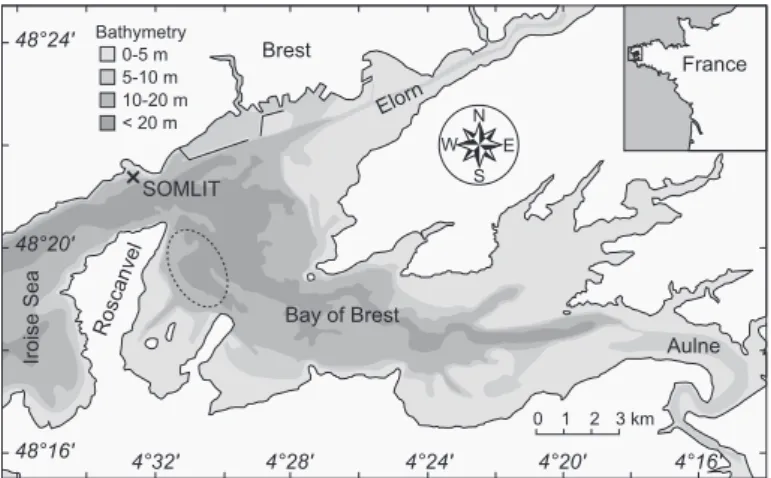
Our study site, the Roscanvel bank, is located in the bay of Brest (Brittany, northwest France; Figure 2), a semi-enclosed marine ecosystem of 180 km2connected to shelf waters (Iroise Sea) by a narrow and deep strait (2 km width, 40 m depth). This bay is a shallow basin with an aver-age depth of 8 m. Two rivers, the Aulne (catchment area = 1792 km2) and the Elorn (catchment area = 379 km2), are responsible for up to 80% of the total freshwater input in the bay. Both catchements are composed of protero-zoic and palaeoprotero-zoic sedimentary rocks (shales and sand-stones), punctuated with some more recent granite intru-sions. Tidal amplitudes reach 8 m during spring tides, re-sulting in an oscillating volume that is 40% of the high tide volume; this induces short-term variability in hydrographic parameters and mixing of water masses (Chauvaud et al., 2005). Brest 4°32' 4°28' 4°24' 4°20' 4°16' E N W S 0 1 2 3 km 48°16' 48°24' 48°20'
Roscanvel Bay of Brest
Iroise Sea SOMLIT 0-5 m 5-10 m 10-20 m < 20 m Bathymetry France Aulne Elorn
Figure 2: Shell sampling location in the Bay of Brest, north-west France (Roscanvel bank: dashed ellipse) and SOMLIT-Brest water monitoring station (black cross).
The Roscanvel bank (30 m water depth), is located in the western part of the bay of Brest (Figure 2). It is charac-terized by mixed sandy and silty sediments, and is known to host a large population of great scallop Pecten maximus. The Roscanvel bank has marine characteristics as bottom-water salinity only decreases down to 32.5 during winter flood tides, whereas it is quite stable (34–35) from spring to fall, ie. when scallops accrete calcite (Chauvaud et al., 1998).
2.2. Environmental parameters
Environmental parameters were monitored weekly from 1999 to 2007 at the SOMLIT-Brest station located at the outlet of the bay (Figure 2). Water sampling and mea-surements were performed at 1 m depth at slack high tide in mean tidal conditions, in order to favour the oceanic sig-nal more than the influence of riverine inputs. Temperature and salinity were measured with a Sea-Bird SBE 19 CTD profiler (Sea-Bird Electronics, Inc.). For the determination of chlorophyll a concentration, 1 L of seawater collected us-ing a Niskin bottle was filtered onto Whatmann GF/F fil-ters. The analysis was done according to Yentsch and Men-zel (1963) using a calibrated Turner 111 fluorometer. Wa-ter samples for phytoplankton species deWa-termination were preserved in Lugol’s solution. Species were identified and counted by examination on an inverted microscope. Un-fortunately, no information is available on phytoplankton community composition over the period 2005–2007, thus preventing comparison of Li/Cashellwith in situ biological data.
Temperature and salinity measured at SOMLIT-Brest are known to reflect very precisely environmental conditions at Roscanvel bank (Lorrain, 2002). On another hand, there are some differences in the composition of phytoplankton communities and timing of blooms between both stations; if blooms of dominant diatom and dinoflagellate species occur approximately at the same time at SOMLIT-Brest and Roscanvel, their intensities could differ significantly. More-over, many minor species observed at SOMLIT-Brest are typically oceanic and are not found at Roscanvel. Conse-quently, we only considered cell counts for diatom species (i) that are known to be dominant species at Roscanvel (Chauvaud et al., 1998; Lorrain et al., 2000), and (ii) that rep-resented more than 10% of total diatom counts at SOMLIT-Brest over the period 1999–2004. The same strategy was applied to dinoflagellates. Therefore, we used counts of Chaetoceros spp. (30% of total diatoms), Dactyliosolen frag-ilissimus (formerly Rhizosolenia fragilissima; 10%), Guinar-dia delicatula (formerly Rhizosolenia delicatula; 17%), and Pseudo-nitzschia spp. (10%). All together, these species represented two thirds of diatoms counted at SOMLIT-Brest between 1999 and 2004. As for dinoflagellates, Gymno-dinium spp. represented 60% of total dinoflagellates be-tween 1999 and 2004.
2.3. Shell sampling and growth measurements
Live scallops were collected from Roscanvel bank using SCUBA diving. Individuals of age class I (ie. specimens that have lived only one 1stof January) were sampled on 21 November 2001 (n = 3 shells born in 2000), on 3 September 2004 (n = 3 shells born in 2003) and on 5 November 2007 (n
= 4 shells born in 2006). For all these specimens, we anal-ysed the part of the shell between the first winter growth mark and the ventral margin. This portion corresponded to shell material formed in 2001, 2004, and 2007, respectively (ie. during the second year of growth). In addition, age class III specimens were collected on 23 March 2001 (n = 3 shells born in 1998). For these three individuals, we anal-ysed shell material located between the first and the second winter growth mark, ie. calcite formed in 1999. Analysis of shell material formed between the first and the second winter growth mark was chosen because this second year of growth corresponds to the longest annual growth season, and thus provides the longest annual calcitic record (Figure 1). In the bay of Brest, scallops in their second year grow from late March-early April to November (Chauvaud et al., 1998).
Before shell growth and elemental analyses, the upper surface of the left valves was cleaned by soaking for 3 min-utes in 90% acetic acid. They were then rinsed by deion-ized water and air-dried. Daily shell growth rates (DSGR) were determined by measuring distances between succes-sive daily growth striae along the axis of maximum growth using the image analysis method described by Chauvaud et al. (1998). On the basis of the daily rhythm of striae for-mation, absolute dates of precipitation were assigned to each stria by backdating from the last deposited stria at the day of collection (see Chauvaud et al. (2005) for elabora-tion).
2.4. Elemental analyses
Using a micromilling device (New Wave Research) equipped with a 300-µm tungsten carbide drill bit, calcite powder was milled directly from the upper surface of the left valve of the shells, along the axis of maximum growth. One stria was milled every three striae, a sampling strat-egy corresponding to ca. two calcite samples per week of shell growth (sub-weekly resolution). Sample prepara-tion and analyses were performed at the Pôle Spectrométrie Océan (Plouzané, France). All samples were prepared in a class 10000 clean laboratory. Ultra-pure deionized wa-ter (resistivity = 18.2 MΩ.cm) was used for mawa-terial clean-ing and acid dilutions. Nitric acid solutions (commercial grade, Merck) were purified by distillation in sub-boiling silica glass stills (Quartex). All material (polypropylene cen-trifuge tubes, disposable pipette tips, etc.) was pre-cleaned using 5% HNO3and rinsed with ultra-pure deionized water. A known weight of each shell sample (average weight = 127 µg) was transferred into a pre-cleaned polypropylene centrifuge tube, dissolved in 2% HNO3, and spiked with a known amount (about 7 µL) of a mono-elemental thulium solution (Tm concentration = 77.9 ng g-1). Thulium was used as an internal standard to correct short- and long-term instrumental drift (see Barrat et al. (1996) and Bayon et al. (2009) for detailed information on this method). Ex-ternal calibration was performed using an in-house multi-element solution prepared from certified stock solutions. This calibration solution was prepared so that it closely matched the calcium carbonate matrix and elemental com-position of mollusc shells.
Elemental concentrations were measured on a Thermo Electron Element2 high-resolution inductively coupled
plasma mass spectrometer equipped with an ASX 260 auto-sampler (CETAC Technologies). Solutions were introduced via a Teflon nebulizer and a Peltier cooled cyclonic spray chamber. The Element2 was equipped with a glass injec-tor and a set of nickel sampler and skimmer cones. Along the course of this study, plasma power ranged between 1270 and 1310 W and argon flow rates were 16.06 L min-1(cooling gas), 0.54–0.65 L min-1(auxiliary gas), and 0.95–1.35 L min-1 (nebulizer gas). The Element2 was operated in medium resolution (m/∆m = 4000) and measured isotopes were7Li and43Ca (among other elements not presented in this arti-cle). Concentrations were calculated using the Tm addition method. Details on the calculations can be found in Bayon et al. (2009). Briefly, for each sample, elemental concentra-tions were calculated using the sample mass, the amount of Tm added, and by calibrating the raw data acquired during the measurement session against the unspiked (no added Tm) in-house multi-element solution, run after every five samples.
Precision (degree of reproducibility) and accuracy (de-gree of veracity) of our procedure were controlled through analyses of (i) a certified reference material purchased from the National Research Council of Canada (FEBS-1: red snapper Lutjanus campechanus saggital otolith; certified values in Sturgeon et al., 2005), and (ii) a Pecten maximus in-house reference material (left valve of a specimen from the bay of Brest, crushed and carefully homogenized). Re-peated measurements of these reference materials yielded a precision (relative standard deviation) of 2.05% (average Li/CaFEBS-1 = 4.32 µmol mol-1; 1σ = 0.09 µmol mol-1; n = 12) and 7.76% (average Li/CaPecten = 22.50 µmol mol-1; 1σ = 1.75 µmol mol-1; n = 109). Accuracy was extremely good with a Li concentration value in FEBS-1 of 0.304± 0.007 mg kg-1(mean± standard deviation) compared with the rec-ommended value of 0.305 ± 0.044 mg kg-1. Our method slightly overestimated Ca concentration (+ 6%) with a mea-sured value in FEBS-1 of 407 000± 9 000 mg kg-1 (mean ± standard deviation) compared with the recommended value of 383 000± 14 000 mg kg-1.
In order to check the reproducibility of Li/Cashellratios along a given shell, one specimen collected on 5 Novem-ber 2007 (shell #6) was also analysed for elemental content along three different axes of shell growth: the central axis (ie. axis of maximum shell growth), an axis on the left side of the shell, and another one on the right side.
2.5. Statistical analyses
Differences in Li/Cashellratios between left, central and right axes of shell #6 were tested with an analysis of vari-ance after verification of homoscedasticity with Bartlett’s test (α = 0.01). Tukey HSD (Honestly Significant Differ-ence) post-hoc test was used to identify which axis differed from the other ones. Simple and multiple linear regres-sions were performed between Li/Cashell and possible ex-planatory variables (seawater temperature, salinity, chloro-phyllaconcentration, and daily shell growth rate) for each single year (1999, 2001, 2004, and 2007) and for the whole dataset (1999–2007). Before performing multivariate re-gressions, we used the Schwartz’s Bayesian Information Criterion (BIC) to select the best subset of explanatory vari-ables. Finally, a model II regression was used to fit Li/Cashell
6 8 10 12 14 16 18 20 0 1 2 3 4 5 6 7 8 30 31 32 33 34 35 36 Te m perature ( °C) Salinity Chlorophyll a (µ g L -1) 1999 2000 2001 2002 2003 2004 Pseudo-nitzschia sp. Guinardia delicatula Gymnodinium sp. Chaetoceros sp. Dactyliosolen fragilissimus 0 2 4 6 8 0 2 4 6 8 0 2 4 6 8 0 2 4 6 8 0 2 4 6 8 10 5 cell L -1 10 5 cell L -1 10 5 cell L -1 10 5 cell L -1 10 5 cell L -1 2005 2006 2007 1999 2000 2001 2002 2003 2004 2005 2006 2007 No phytoplankton data available over the period
2005-2007
Figure 3: Variations of physical (temperature, salinity) and biological (chlorophyll a concentration, phytoplankton counts) parameters recorded at the SOMLIT-Brest monitoring station from 1999 to 2007. Note that phytoplankton counts are not available between 2005 and 2007.
and DSGR (Standard Major Axis). All statistical analyses were performed with R, using “leaps” (for BIC model selec-tion criteria) and “lmodel2” (for model II regressions) pack-ages.
3. Results
3.1. Variability of environmental parameters between 1999 and 2007
Temperature variations at SOMLIT-Brest displayed a clear seasonal signal over the study period, with an annual temperature range from 8.0°C in 2007 to 10.1°C in 2003 (Fig-ure 3). Water temperat(Fig-ure was lowest between mid-January and mid-March (mean 1999–2007 = 8.8°C; σ = 0.6°C) and reached a maximum in August–September (mean 1999– 2007 = 17.7°C; σ = 0.5°C). Over the same period, there were minor fluctuations in surface salinity, usually ranging be-tween 33 and 35.6. Salinity drops during winter and early spring corresponded with increases in Aulne and Elorn flows. Exceptional surface salinity decreases were recorded in January 2000 (31.7) and January 2001 (32.3). These quite low salinities were likely restricted to surface waters and did not influence scallops in Roscanvel bottom water. Intra-annual salinity ranges varied from 0.97 in 2005 to 3.84 in 2000. These temperature and salinity values were very simi-lar to bottom-water values measured at Roscanvel by Chau-vaud et al. (1998).
Chlorophyll a concentration ranged from 0.12 µg L-1in February 2005 to 6.39 µg L-1in April 2003 (Figure 3). Largest annual phytoplankton blooms were recorded in May, ex-cept in 2002 (maximum concentration in August) and in 2006 (maximum concentration in October), with varying intensities depending on the year (from 2.70 µg L-1in 2004 to 6.39 µg L-1in 2003). The mean chlorophyll a value was 1.2 µg L-1over the study period. This value masked some inter-annual variations, especially in 2002 (highest mean annual concentration of 1.8 µg L-1) and in 2005 (lowest mean annual concentration of 0.6 µg L-1).
Most of this chlorophyll a was contained within cells of the diatom genus Chaetoceros (Figure 3). This genus was present in the water column every year, with concen-trations reaching 634 670 cell L-1 on 22 June 2004. High-est abundances were recorded in 1999 and 2004, whereas 2001 was characterized with only two small blooms (< 250 000 cell L-1). Another abundant diatom, Dactyliosolen frag-ilissimus, displayed important blooms at SOMLIT-Brest in 2003 and 2004 (up to 402 730 cell L-1on 8 June 2004). This species presented very low levels from 1999 to 2002 (< 100 000 cell L-1). The diatom Guinardia delicatula formed large blooms in 1999, 2001, and 2002, up to 653 877 cell L-1(in May 2001), but displayed low levels in 2000, 2003, and 2004 (< 150 000 cell L-1). The fourth genus of diatoms abundant at SOMLIT-Brest was Pseudo-nitzschia. These species were usually not present in the water column, except in July 2000 and in May 2004 when they formed a very large bloom up to 822 931 cell L-1. One dinoflagellate genus, Gymnodinium, presented quite high levels between 1999 and 2002, with two large blooms in late August (773 478 cell L-1) and mid-October 2001 (486 388 cell L-1). It should be mentioned that another dinoflagellate species, Karenia mikimotoi (for-merly Gymnodinium nagasakiense), represented 23% of to-tal dinoflagellates at SOMLIT-Brest, because of a unique
large bloom in August 2002 (678 321 cell L-1). Finally, max-imum chlorophyll a concentrations recorded in 2000 and 2003 were related to diatom blooms of Thalassiosira spp. (196 997 cell L-1 on 2 May 2000; 5% of total diatoms at SOMLIT-Brest) and Cerataulina pelagica (444 357 cell L-1on 28 April 2003; 4% of total diatoms).
0 10 20 30 40 50 60 70
Mar Apr May Jun Jul Aug Sep Oct
Year 2007
Li/Cashell (left) Li/Cashell (center) Li/Cashell (right)
Li/Ca shell ( µ mol mol -1)
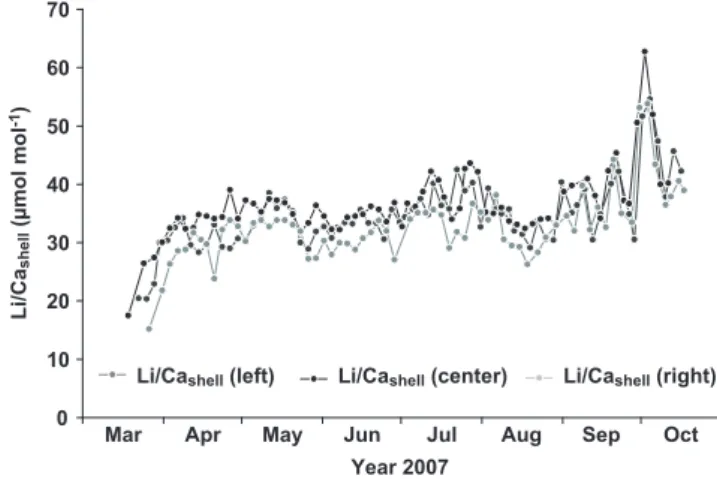
Figure 4: Temporal variations of Li/Ca ratios along left, cen-tral, and right axes of growth of shell #6 collected on 5 November 2007.
3.2. Li/Cashelltime series and daily shell growth rate
Li/Cashellratio time series along the three axes of growth were remarkably similar, with highest ratios recorded at the same time between 2 October 2007 and 4 October 2007 (Figure 4). Average Li/Cashellratio on left, central, and right axis were 34.54 µmol mol-1 (σ = 5.81 µmol mol-1), 36.40 µmol mol-1(σ = 5.83 µmol mol-1), and 32.79 µmol mol-1(σ = 5.86 µmol mol-1), respectively. These small differences were statistically significant (Bartlett’s test: χ2Bartlett= 0.006, df = 2, p = 0.997; ANOVA: F = 6.56, df = 2 and 206, p = 0.002); post-hoc test indicated that average Li/Cashell ratio on the right axis was significantly lower than on the central axis.
Temporal variations of Li/Cashelldisplayed a high degree of synchronism (inter-individual reproducibility), whatever the year (Figure 5). On another hand, Li/Cashellshowed very different trajectories in 1999, 2004, and in 2001 and 2007. In 1999, all three specimens presented a kind of exponen-tial increase in Li/Cashellfrom ca. 20 µmol mol-1in March to 190–250 µmol mol-1 (depending on the specimen) be-tween 2 July 1999 and 4 July 1999. Li/Cashellthen decreased down to values around 30–40 µmol mol-1at the end of July and stayed at this level until December. In 2004, Li/Cashell presented values around 30–40 µmol mol-1, except from the end of May to the end of July. During that period, all three specimens displayed a high degree of synchronism, presenting the same profiles punctuated with three main Li/Cashellpeaks at the beginning of June (90–95 µmol mol-1), at the end of June (90–100 µmol mol-1), and in mid-July (65– 75 µmol mol-1). In 2001 and 2007, Li/Ca
shell values
fluctu-ated between 15 and 50 µmol mol-1 all year long, except a little sharp peak around 65–70 µmol mol-1at the begin-ning of October 2007 on the four studied specimens. Given the very low inter-individual variability in Li/Cashelland the sharpness of Li/Cashell peaks, it is likely that the latter re-sulted from transient phenomenons in the water column (environmental forcing).
Table 1: Annual minimum, maximum, and mean values of Li/Cashelland daily shell growth rate of each Pecten maximus specimen analyzed over the period 1999–2007.
Year Shell Li/Cashell(µmol mol-1) DSGR (µm d-1)
Min. Mean Max. Min. Mean Max.
1999 #103 19.05 50.03 243.83 40.66 202.32 329.29 #105 17.02 50.79 191.22 86.17 229.91 377.09 #106 16.48 48.53 202.28 45.08 176.69 307.64 2001 #5 14.87 28.86 43.09 42.17 176.34 298.25 #10 19.90 32.01 48.53 57.52 176.29 262.42 #12 20.24 34.87 47.22 53.44 177.37 274.62 2004 #1 15.19 47.89 93.41 37.11 227.82 340.16 #2 18.39 47.94 90.43 36.88 244.44 385.60 #3 21.14 50.83 100.96 61.47 228.24 409.84 2007 #5 15.64 35.97 63.53 68.17 213.06 377.27 #7 18.32 34.51 70.01 30.98 167.84 290.74 #666 18.49 35.18 70.09 47.11 177.98 285.14 #6 17.49 36.40 62.74 42.43 166.19 306.47
Daily shell growth rate varied by an order of magnitude over a given growing season from minima around 35–50 µm d-1to maxima reaching 250–350 µm d-1, with very lit-tle inter-individual variability (Figure 5). Whatever the year, shell growth restarted at the end of March after a winter growth cessation, and reached maximum values in June-July. Significant differences were observed in shell growth trajectories between years. In 1999, scallops exhibited a sharp increase in DSGR from March to July, and then a slow decrease until the following winter growth cessation. Shell growth, however, was abruptly reduced in May 1999 (-75 µm d-1). In 2001, shell growth slightly increased from March to mid-May, suddenly dropped down to ca. 90 µm
d-1at the end of May, abruptly increased to reach maxima in July, and then slowly decreased until November. The lat-ter decrease was punctuated with a growth retardation in September 2001. Shell growth trajectory was quite similar in 2001 and 2004, at least until the end of August. No data were available after August 2004 as shells were collected be-fore the end of the growing season. Finally, in 2007, DSGR sharply increased from 35 µm d-1in March to ca. 220 µm d-1in April, and stayed around 150–250 µm d-1until Octo-ber (except at the end of May 2007 when a sudden decrease down to 100 µm d-1was observed). Note that all geochemi-cal and shell growth data obtained on each of the 13 speci-mens analysed in this study can be retrieved in Table 1. Table 2: Summary of simple and multiple linear regressions performed with Li/Cashellas response variable, and seawater temperature, salinity, chlorophyll a concentration and daily shell growth rate as explanatory variables.
Estimate Std. error T p-value F -statistic Adjustedr2 p-value
Year 1999 Temperature 3.57 2.83 1.261 0.216 1.59 on 1 and 32df 0.018 0.216 Intercept -3.57 43.58 -0.082 0.935 Salinity -6.44 17.21 -0.374 0.711 0.14 on 1 and 32df -0.027 0.711 Intercept 274.36 597.17 0.459 0.649 Chlorophylla 9.52 6.45 1.475 0.150 2.18 on 1 and 32df 0.034 0.150 Intercept 37.23 11.01 3.382 0.002 DSGR 0.40 0.10 4.113 < 0.001 16.92 on 1 and 32df 0.325 < 0.001 Intercept -24.92 19.09 -1.305 0.201 DSGR 0.55 0.13 4.286 < 0.001 10.41 on 2 and 31df 0.363 < 0.001 Temperature -5.22 3.06 -1.703 0.099 Intercept 27.25 35.81 0.761 0.452 Year 2001 Temperature 2.05 0.33 6.255 < 0.001 39.12 on 1 and 30df 0.552 < 0.001 Intercept 0.53 4.99 0.107 0.916 Salinity 6.64 1.24 5.380 < 0.001 28.94 on 1 and 30df 0.474 < 0.001 Intercept -199.19 42.89 -4.644 < 0.001 Chlorophylla -0.25 0.91 -0.279 0.782 0.078 on 1 and 30df -0.031 0.782 Intercept 32.00 2.09 15.289 < 0.001
Table 2 – Continued from previous page
Estimate Std. error T p-value F -statistic Adjustedr2 p-value
DSGR 0.10 0.01 9.021 < 0.001 81.38 on 1 and 30df 0.722 < 0.001 Intercept 14.64 1.94 7.533 < 0.001 DSGR 0.08 0.01 5.533 < 0.001 44.06 on 2 and 29df 0.735 < 0.001 Salinity 1.95 1.22 1.595 0.122 Intercept -50.11 40.64 -1.233 0.228 Year 2004 Temperature 3.94 1.39 2.826 0.010 7.99 on 1 and 20df 0.250 0.010 Intercept -8.12 20.13 -0.403 0.691 Salinity 16.70 8.06 2.072 0.051 4.30 on 1 and 20df 0.136 0.051 Intercept -528.31 278.03 -1.900 0.072 Chlorophylla 12.94 9.04 1.432 0.167 2.05 on 1 and 21df 0.046 0.167 Intercept 32.46 11.31 2.871 0.009 DSGR 0.18 0.05 3.638 0.002 13.23 on 1 and 21df 0.357 0.002 Intercept 6.94 11.65 0.596 0.558 DSGR 0.45 0.12 3.862 0.001 11.10 on 2 and 19df 0.490 < 0.001 Salinity -40.19 15.98 -2.516 0.021 Intercept 1332.06 526.90 2.528 0.020 Year 2007 Temperature 1.50 0.68 2.199 0.037 4.83 on 1 and 25df 0.129 0.037 Intercept 13.44 10.28 1.307 0.203 Salinity 19.07 4.69 4.064 < 0.001 16.52 on 1 and 25df 0.374 < 0.001 Intercept -628.31 163.42 -3.845 < 0.001 Chlorophylla -3.96 1.76 -2.254 0.033 5.08 on 1 and 25df 0.136 0.033 Intercept 41.62 2.89 14.427 < 0.001 DSGR 0.07 0.03 2.146 0.042 4.60 on 1 and 25df 0.122 0.042 Intercept 23.92 5.72 4.181 < 0.001 DSGR 0.05 0.03 2.087 0.048 11.55 on 2 and 24df 0.448 < 0.001 Salinity 17.69 4.46 3.971 < 0.001 Intercept -589.57 154.56 -3.815 < 0.001 Years 1999–2007 Temperature 2.73 0.94 2.911 0.004 8.48 on 1 and 113df 0.062 0.004 Intercept 0.62 14.15 0.044 0.965 Salinity 4.45 4.71 0.944 0.347 0.89 on 1 and 113df -0.001 0.347 Intercept -112.90 163.50 -0.691 0.491 Chlorophylla 0.40 2.29 0.173 0.863 0.03 on 1 and 114df -0.009 0.863 Intercept 40.77 4.13 9.882 < 0.001 DSGR 0.21 0.03 6.539 < 0.001 42.76 on 1 and 114df 0.266 < 0.001 Intercept 1.42 6.38 0.223 0.824 DSGR 0.24 0.04 6.678 < 0.001 22.92 on 2 and 112df 0.278 < 0.001 Salinity -7.29 4.37 -1.668 0.098 Intercept 249.99 149.14 1.676 0.097
3.3. Multivariate statistical analyses of Li/Cashellvariations Simple and multiple linear regressions provided inter-esting information on variables that may explain Li/Cashell variations (Table 2). As inter-individual variability in Li/Cashelltime series was very low for a given growing sea-son (Figure 5), we calculated average Li/Cashellprofiles for each year. Simple regressions performed on each year in-dicated that the variable with the strongest statistically sig-nificant (p < 0.05) relationship with average Li/Cashellwas DSGR in 1999 (r2= 0.325), in 2001 (r2= 0.722), and in 2004 (r2 = 0.357), and salinity in 2007 (r2 = 0.374). Except in 2007 (r2= 0.136; p = 0.033), chlorophyll a concentration did not present a significant relationship with Li/Cashell. Sea-water temperature relationship with Li/Cashell was strong in 2001 (r2 = 0.552; p < 0.001), weak albeit significant in
2004 (r2= 0.250; p = 0.01) and 2007 (r2= 0.129; p = 0.037), and non-significant in 1999 (r2= 0.018; p = 0.216). Multi-ple linear regressions performed for each year with the two best explanatory variables (selected using the Schwartz’s Bayesian Information Criterion: DSGR and temperature in 1999; DSGR and salinity in 2001, 2004, and 2007) were all statistically significant (p < 0.001). However, the only vari-able that was always statistically significant in these mod-els was DSGR (together with salinity in 2004 and 2007). These models explained between 36.3 and 49.0% of aver-age Li/Cashellvariability in 1999, 2004 and 2007, suggesting that most of this variability resulted from another param-eter (see discussion below on phytoplankton species). On another hand, our multivariate model explained 73.5% of Li/Cashell variability in 2001, ie. when no Li/Cashell peaks
Li/Ca shell ( µ mol mol -1)
Daily shell growth rate (
µ m d -1) 0 50 100 150 200 250 0 100 200 300 400
Mar Apr May Jun Jul Aug Sep
Year 2004 0 50 100 150 200 250 0 100 200 300 400
Mar Apr May Jun Jul Aug Dec
Year 2001
Sep Oct Nov
Li/Ca shell ( µ mol mol -1)
Daily shell growth rate (
µ m d -1) 0 50 100 150 200 250 0 100 200 300 400
Mar Apr May Jun Jul Aug Dec
Year 1999
Sep Oct Nov
Li/Ca shell ( µ mol mol -1)
Daily shell growth rate (
µ m d -1) 0 50 100 150 200 250 0 100 200 300 400
Mar Apr May Jun Jul Aug Sep Oct
Year 2007 Li/Ca shell ( µ mol mol -1)
Daily shell growth rate (
µ
m d
-1)
Daily shell growth rate
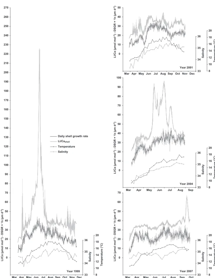
Figure 5: Time series of Li/Cashell(greyscale symbols) and average daily shell growth rate (black line;± 1 standard error) in 1999 (n = 3 shells), 2001 (n = 3), 2004 (n = 3), and 2007 (n = 4).
were recorded in the shells. Most of this variability was ex-plained by DSGR as salinity was not a significant predic-tor in this model (p = 0.122). When all years were con-sidered as a single dataset covering the period 1999–2007, the only variables that significantly explained some part of the Li/Cashell variability were DSGR (r2= 0.266; p < 0.001) and, to a lesser extent, seawater temperature (r2= 0.062; p = 0.004).
Graphical outputs confirmed results of these statistical analyses. Average Li/Cashellprofiles are displayed on Figure 6, together with average DSGR and seasonal variations of seawater temperature and salinity, ie. the three variables that could most likely explain variations of Li/Cashell (see Table 2). We increased the vertical resolution of the y-axis in comparison with Figure 5 in order to get a better insight of baseline variations of Li/Cashell time series. It appeared clearly that Li/Cashellpeaks were not induced by variations of DSGR, temperature or salinity. None of these parameters presented sharp increases or decreases synchronous with Li/Cashell peaks (Figure 6). Therefore, the statistically sig-nificant relationships described between average Li/Cashell variations on one hand, and DSGR, temperature or salin-ity on the other hand, very likely pertained to variations of baseline Li/Cashell. Outside peak periods, variations of baseline Li/Cashelltended to follow the same pattern as sea-sonal variations of DSGR. This was particularly striking for shells collected in November 2001 and, to a lesser extent, in November 2007 (part of the time series between March and September 2007, ie. before the early October Li/Cashell peak). This growth–Li/Cashell relationship was also visible on 1999 and 2004 shells, between March and May 1999, be-tween August and December 1999, and from March to May 2004 (ie. outside the peak periods). Cross-plots of Li/Cashell
versus DSGR, established for each year, confirmed these observations (Figure 7). In 2001, ie. the year when shells did not present Li/Cashellpeaks, Li/Cashelland DSGR presented a strong and highly significant relationship (Standard Ma-jor Axis regression, n = 237, r = 0.86, p < 0.001; Figure 7). In 1999, 2004, and to a lesser extent 2007, growth–Li/Cashell relationships, although statistically significant (p < 0.001), were weaker (r ≤ 0.64) and deviated from the relationship established in 2001. Slopes of these relationships (0.160≤ slope≤ 0.550) were higher than in 2001 (slope = 0.107), re-flecting the presence of Li/Cashellpeaks in 1999, 2004, and 2007 (Figure 7).
On another hand, no obvious relationship was observed between variations of baseline Li/Cashell and variations of temperature and salinity (Figure 7). This was especially noticeable in May 2001 when Li/Cashelldecreased abruptly whereas temperature and salinity did not present any sig-nificant decrease nor abrupt increase. This confirmed equivocal results of simple and multiple linear regressions between Li/Cashell and these two environmental variables (Table 2).
3.4. Variations of excess Li/Cashell
In order to investigate determinism of Li/Cashell peaks, we made the assumption that Li/Cashell variations were mostly controlled by DSGR outside peak periods (which was confirmed by statistical analyses and graphical out-puts; Table 2 and Figures 6–7). We selected data obtained on shells collected in November 2001, that did not present Li/Cashellpeaks, to derive the growth–baseline Li/Cashell re-lationship:
Year 2001 Year 2004 Year 2007 0 10 20 30 40 50 Li/Ca ( µ mol mol -1) - DSGR × 1/8 (µ m d -1)
Mar Apr May Jun Jul Aug Sep Oct Nov Dec 33
34 35 36 Salinity 8 10 12 14 16 18 20 Temperature ( °C) 0 10 20 30 40 50 70 80 90 60 100 Li/Ca ( µ mol mol -1) - DSGR × 1/8 ( µ m d -1)
Mar Apr May Jun Jul Aug Sep 33
34 35 36 Salinity 8 10 12 14 16 18 20 Temperature ( °C) 0 10 20 30 40 50 70 60 Li/Ca ( µ mol mol -1) - DSGR × 1/8 ( µ m d -1)
Mar Apr May Jun Jul Aug Sep Oct 33
34 35 36 Salinity 8 10 12 14 16 18 20 Temperature ( °C)
Daily shell growth rate
Li/Cashell Temperature Salinity Year 1999 0 10 20 30 40 50 60 70 80 90 100 110 120 130 150 140 200 190 180 170 160 210 240 230 220 250 Li/Ca ( µ mol mol -1) - DSGR × 1/8 ( µ m d -1)
Mar Apr May Jun Jul Aug Sep Oct Nov Dec 33
34 35 36 Salinity 8 10 12 14 16 18 20 Temperature ( °C) 260 270
Figure 6: Time series of average Li/Cashell(grey line;± 1 standard error), average daily shell growth rate (DSGR; black line; ± 1 standard error), seawater temperature (black dotted line) and salinity (grey dotted line) in 1999 (n = 3 shells), 2001 (n = 3), 2004 (n = 3), and 2007 (n = 4), revealing co-variations of shell growth and baseline Li/Cashell.
0 50 100
0 100 200 300 400
Daily shell growth rate (µm d-1)
Li/Ca shell ( µ mol mol -1) 0 50 100 0 100 200 300 400 Li/Ca shell ( µ mol mol -1)
Daily shell growth rate (µm d-1)
0 0 100 200 300 400 50 100 Li/Ca shell ( µ mol mol -1)
Daily shell growth rate (µm d-1)
0 50 100 150 200 250 0 100 200 300 400 Li/Ca shell ( µ mol mol -1)
Daily shell growth rate (µm d-1)
Year 1999
Year 2001
Year 2004
Year 2007
Li/Cashell = 0.550 × Growth - 55.879
(r = 0.64; p < 0.001)
Li/Cashell = 0.107 × Growth + 12.824
(r = 0.86; p < 0.001)
Li/Cashell = 0.305 × Growth - 21.539
(r = 0.62; p < 0.001)
Li/Cashell = 0.160 × Growth + 6.667
(r = 0.45; p < 0.001) 2001 2007 2001 2004 2001 1999 Pecten maximus Arctica islandica
Figure 7: Cross-plots of average Li/Ca versus daily shell growth rate for years 1999, 2001, 2004, and 2007. Model II regression lines (SMA; black dashed line) are presented to-gether with regression statistics. For comparative purposes, (i) 2001 SMA regression line is displayed on cross-plots for years 1999, 2004, and 2007 (grey dotted lines), and (ii) Li/Ca versus daily shell growth rate regression line calculated for Arctica islandica (Thébault et al., 2009b) is presented on the 2001 cross-plot (grey dotted line).
Then, we predicted Li/Cashell variations for each year using average daily shell growth data and Equation 1, as-suming that baseline Li/Cashellvariations were only caused by variations in DSGR. Time series of the difference be-tween predicted and observed Li/Cashell, so-called excess Li/Cashell (Li/Caexcess), are displayed on Figure 8, together with DSGR and phytoplankton abundances (except for year 2007 when no phytoplankton data were available). Phyto-plankton species were split into two groups: (i) edible di-atoms (Chaetoceros spp. and Dactyliosolen fragilissimus), ie. diatoms that have no negative influence on scallop growth in the bay of Brest, and (ii) toxic (Gymnodinium spp., harmful dinoflagellates responsible for red tides; Landsberg, 2002) and aggregate-forming or chain-forming species (Guinardia delicatula and Pseudo-nitzschia spp.) that can hamper scallop growth (Chauvaud et al., 1998; Lor-rain et al., 2000; Nézan et al., 2010).
Temporal variations of edible diatom abundance tended to mimic those of Li/Caexcess, with a time lag of ca. 3 weeks (Figure 8, upper panels). This was particu-larly striking in 2004 (proportionality between Li/Caexcess and edible diatom peaks). In 1999, intensity of the edible diatom bloom recorded at SOMLIT-Brest was close to 500 000 cell L-1on 10 June 1999; this did not seem sufficient to induce the large Li/Caexcesspeak recorded in early July 1999. However, this bloom was much larger on Roscanvel Bank than at SOMLIT-Brest, as indicated by the environmental survey performed by Lorrain et al. (2000) in 1999 exactly where our scallops were collected (9 June 1999: 1 458 000 cell Chaetoceros spp. L-1). On the other hand, neither large edible diatom bloom nor Li/Caexcesspeak were observed in 2001.
3.5. Relationship between shell growth retardation and phy-toplankton blooms
Several growth retardation episodes were recorded on 1999, 2001, and 2004 shells (Figure 8, lower panels). In 1999 and 2001, main accidents always occurred a few days after blooms of Guinardia delicatula (May 1999 and May 2001) and Gymnodinium spp. (September 2001). Some toxic blooms, however, did not seem to hamper shell growth (Au-gust 1999 and October 2001). In 2004, a severe growth retar-dation was observed but was not preceded by a bloom. Fi-nally, a very large bloom of Pseudo-nitzschia spp. occurred on 24 May 2004 (> 800 000 cell L-1), ie. 2 weeks after the growth accident. It should be kept in mind, however, that the timing of blooms may be slightly different at SOMLIT-Brest and Roscanvel.
4. Discussion
Lithium content has rarely been investigated in marine biogenic carbonates in comparison with other elements such as Mg, Sr, or Ba. Most studies on Li/Ca ratio in bio-carbonates dealt with foraminifera (Delaney et al., 1985; Delaney and Boyle, 1986; Hall and Chan, 2004; Marriott et al., 2004b; Hathorne and James, 2006; Lear and Rosen-thal, 2006; Hendry et al., 2009; Lear et al., 2010), and to a lesser extent with corals (Marriott et al., 2004a; Montagna et al., 2006) and brachiopods (Delaney et al., 1989). The
0 20 40 60 80 100 120 140 160 180 0 3 6 9 12 15 0 20 40 60 80 100 120 140 160 180 0 3 6 9 12 15 0 20 40 60 80 100 120 140 160 180 0 3 6 9 12 15 Mar Apr May Jun Jul Aug Sep Oct Nov Dec Mar Apr May Jun Jul Aug Sep Oct Nov Dec Mar Apr May Jun Jul Aug Sep Excess Li/Ca shell (µ mol mol -1 ) Phytoplankton (10 5 cell L -1 ) Phytoplankton (10 5 cell L -1 ) Phytoplankton (10 5 cell L -1 ) Mar Apr May Jun Jul Aug Sep Oct Nov Dec
Daily shell growth rate (µ m d -1 ) 0 2 4 6 8 10 0 100 200 300 400 Phytoplankton (10 5 cell L -1 ) Mar Apr May Jun Jul Aug Sep Oct Nov Dec 0 100 200 300 400 0 2 4 6 8 10 Phytoplankton (10 5 cell L -1 )
Daily shell growth rate (µ m d -1 ) Mar Apr May Jun Jul Aug Sep 0 100 200 300 400 0 2 4 6 8 10 Phytoplankton (10 5 cell L -1 )
Daily shell growth rate (µ m d -1 ) Excess Li/Ca shell (µ mol mol -1 ) Excess Li/Ca shell (µ mol mol -1 ) Thalassiosira sp. (02/04/1999) Chaetoceros sp. (09/06/1999: 1 458 000 cell L -1)
Daily shell growth rate Guinardia delicatula Pseudo-nitzschia sp. Gymnodinium sp.
Year 1999 Year 2001 Year 2004 Year 1999 Year 2001 Year 2004 Excess Li/Ca shell
Edible diatoms: - Chaetoceros sp. - D. fragilissimus
Figure 8: Upper panels: time series of Li/Caexcess(black line) and counts of edible diatoms measured at SOMLIT-Brest (solid circles; Chaetoceros spp. + Dactyliosolen fragilissimus), for years 1999, 2001, and 2004. Lower panels: time series (1999, 2001, and 2004) of average daily shell growth rate (black line) and abundances of growth-reducing diatoms (solid squares = Guinardia delicatula; solid triangles = Pseudo-nitzschia spp.) and dinoflagellates (light gray crosses = Gymno-dinium spp.).
only known study on Li/Ca ratio in bivalve mollusc shells was conducted on juvenile Arctica islandica shells from northeast Iceland (Thébault et al., 2009b). Given the very low inter-individual variability in Li/Cashellfor a given sea-son of growth (Figures 5 and 6), it is likely that this ratio responds either to variations of one (or several) environ-mental parameter(s), and/or to variations of a physiologi-cal process synchronized within a given population. Previ-ous studies put forward several hypotheses to explain vari-ations of Li/Ca ratio in calcite: influence of calcification temperature, salinity, dissolved Li concentration in seawa-ter, river inputs of Li-rich silicate particles, calcification rate and seawater carbonate ion (CO32-) concentration. In the following paragraphs, we discuss the merits of these hypotheses to explain temporal variability of Li/Cashell in Pecten maximus. A new hypothesis, related to phytoplank-ton blooms, will address the formation of Li/Cashellpeaks. 4.1. Calcification temperature
Many authors highlighted inverse relationships be-tween calcification temperature and Li/Ca in coralline aragonite (Marriott et al., 2004a; Montagna et al., 2006), in foraminifera (Hall and Chan, 2004; Marriott et al., 2004b), in brachiopods (Delaney et al., 1989), as well as in inorganic calcite (Marriott et al., 2004a). Surprisingly, these results are in contradiction with thermodynamic calculations stat-ing that Li content in calcium carbonate should increase with increasing temperature (Hall and Chan, 2004). Con-versely, recent studies on foraminifera and aragonitic bi-valve shells found a positive dependance of Li/Cashell on temperature (Hendry et al., 2009; Thébault et al., 2009b). Simple and multiple linear regressions performed on the whole dataset (1999–2007) indicated that seawater temper-ature alone explained only 6.2% of the Li/Cashellvariability (r2= 0.062; p = 0.004; slope = 2.73; Table 2). In addition, no thermal anomaly, either positive or negative, was observed synchronously with abrupt Li/Cashellincreases, suggesting that temperature did not induce Li/Cashellpeaks (Figure 6). In 2001, ie. a year without Li/Cashellpeaks, temperature ap-peared quite strongly related with Li/Cashell(r2= 0.552; p < 0.001) but thorough observation of Figure 6 indicated that this statistical relationship was not obvious (e.g. in May 2001). It is clear from our results that seawater temperature in the bay of Brest was not the primary factor explaining variations of Li/Cashellbetween 1999 and 2007. Therefore, we conclude that calcification temperature has only a weak positive influence on Li incorporation in Pecten maximus shell calcite precipitated between 8 and 18°C, thus confirm-ing observations by Thébault et al. (2009b) on juvenile Arc-tica islandica.
4.2. Salinity and dissolved lithium concentration
Salinity was put forward as a possible explanation for variations of Li/Ca in inorganic calcite; a salinity decrease, induced by dilution, from 50 to 10 led to a four-fold de-crease in Li/Cacalcite (Marriott et al., 2004b). A similar influence of salinity was also highlighted on Na/Cacalcite and might be general for all alkali metals (Ishikawa and Ichikuni, 1984; Marriott et al., 2004b). Indeed, alkali met-als are known to be incorporated in an interstitial location
in calcite, while they are incorporated in the crystal struc-ture of aragonite in substitution of Ca, leading to forma-tion of Li2CO3crystals (Okumura and Kitano, 1986). Con-sequently, it is their concentration in the calcifying fluid that controls the amount of alkali metals incorporated in-terstitially within calcite, while there is a competition be-tween alkali metals and Ca to enter aragonite so that it is the Li/Ca ratio in the solution which controls Li/Caaragonite. Be-cause Li concentration is approximatley one order of mag-nitude lower in rivers than in seawater (rivers: 0.012 ppm; seawater: 0.180 ppm; Li, 2000), freshwater inputs leading to salinity decrease therefore also induce a decrease of Li concentration in seawater. At SOMLIT-Brest monitoring station, salinity variations were very small between 1999 and 2007, ranging between 33 and 35.6 during the sea-son of growth of Pecten maximus (salinity minima below 33 occurred in winter, when scallops did not grow). Ac-cording to Marriott et al. (2004b), and assuming that bio-genic calcite has the same sensitivity to salinity as inor-ganic calcite, a 1 unit salinity decrease would result in a 3% decrease in Li/Cashell for salinity around 35. There-fore, the salinity range measured at SOMLIT-Brest would be responsible for 8% changes in Li/Cashell, at most. How-ever, average Li/Cashellvariations ranged from 15 to 40 µmol mol-1in 2001, ie. when Li/Ca
shellvariations were the
weak-est. Therefore, salinity, and consequently Li concentra-tion variaconcentra-tions in seawater, cannot be responsible alone for Li/Cashell variations in Pecten maximus. Nevertheless, results of simple and multiple linear regressions, albeit equivocal, suggested that salinity might slightly influence Li/Cashellvariations, in addition to another factor (Table 2). 4.3. Weathered Li-rich particles
In their study on Li/Cashellin juvenile Arctica islandica from northeast Iceland, Thébault et al. (2009b) observed that seasonal variations of the closest river discharge roughly followed the same pattern as Li/Cashell, with max-imum values in June. A direct relationship was highlighted by Gislason et al. (2009) between river discharge and me-chanical weathering of Icelandic basaltic rocks that have a high Li content. Consequently, Thébault et al. (2009b) hypothesized that high loads of Li-rich suspended basaltic particles probably flow to the sea with Icelandic rivers as soon as snow melts. Direct ingestion of these particles, or their weathering on the seafloor after deposition, may be responsible for significant increases in Li content in shells. Could such an hypothesis explain variations of Li/Cashell time series in shells of Pecten maximus? No data are avail-able on lithium concentration in shales and sandstones composing Aulne and Elorn rivers catchments. Assum-ing that these rocks have a high Li content and that they are highly susceptible to mechanical weathering, then high concentrations of Li-rich particles could occurr in the bay of Brest when river flows are at their annual maximum, ie. in January (see figure 4 in Chauvaud et al., 1998). Con-versely, Li-rich particles concentration would be lowest during low water periods, ie. from June to October. Given that highest Li/Cashell values were recorded during these low river levels, it is unlikely that mechanical weathering of river catchments could explain variability of Li/Cashellin
Pecten maximus. This possible explanation can therefore likely be ruled out.
4.4. Calcification rate
Our results distinctly highlighted a statistically signif-icant positive relationship between Li/Cashell and DSGR measured along the axis of maximum growth (Figure 7). This was particularly obvious in 2001 when no Li/Cashell peak occurred (Figures 6 and 7). For years with periods of Li enrichments in shells (1999, 2004, and to a lesser ex-tent 2007), this relationship was still present but partially concealed by the presence of these Li/Cashellpeaks. A simi-lar relationship between Li/Cashelland shell growth was ob-served in Arctica islandica (Thébault et al., 2009b). It is worth noting that the slope of the Li/Cashell–DSGR relation-ship is very similar in both study (0.098 d m-1for aragonitic Arctica islandica vs. 0.107 d m-1 for calcitic Pecten max-imus; Figure 7), suggesting that the control of this physi-ological factor on Li incorporation within bivalve mollusc shells may be general and ubiquitous. This control of shell growth is supported by results of the elemental analyses performed on three different growth axes of shell #6 col-lected on 5 November 2007. Li/Cashellratios displayed very similar temporal variations whatever the growth axis (Fig-ure 4). Nevertheless, average Li/Cashell ratios were signif-icantly higher on the central axis (ie. axis of maximum growth). These differences could likely be explained by the lower daily shell growth rates on lateral ribs in comparison to the median one.
At this point, a clarification must be made about the dif-ference between daily shell growth rate and absolute cal-cification rate. DSGR is not equal to absolute calcal-cification rate (or crystal growth rate) because it does not take into ac-count ontogenetic changes in shell thickness and enlarge-ment. A problem is that crystal growth rate is hardly mea-surable. Lorrain et al. (2004) tried to estimate it more pre-cisely during the second year of growth of Pecten maximus shells from the Bay of Brest by measuring their daily car-bon precipitation rate (DCPR). It appeared than DSGR and DCPR slightly differed. Therefore, it must be kept in mind that DSGR is only an approximation of absolute calcifica-tion rate.
Beside bivalves, several studies also suggested that changes in calcification rate, that could in turn reflect long-term changes in CO32-concentration and carbonate satu-ration state, may be responsible for variations of Li/Ca in foraminiferal calcite (Hall and Chan, 2004; Lear and Rosen-thal, 2006; Hendry et al., 2009). The mechanisms involved in these physiological effects have barely been studied. The influence of calcification rate on Li incorporation in bio-carbonates might be related to the presence of calcifica-tion anomalies. Indeed, Busenberg and Plummer (1985) suggested that the amount of Na incorporated in calcite may be highly dependent on the number of crystal defects, which is in turn favoured by faster growth rates. By analogy, and because Na and Li are both situated in interstitial po-sitions in the calcite crystals (Okumura and Kitano, 1986), it is reasonable to hypothesize that the same effect con-trols Li/Cashell. The faster a shell grows, the more defaults there are in the crystal structure, and the more interstitial
spaces are available for Li inclusions. Concurrent measure-ments of Li/Cashell and scanning electron microscope ob-servations of crystal fabrics in the same shell might help confirming this hypothesis. In any case, our results sug-gested that Li/Cashell was probably controlled by calcifica-tion rate (as estimated by DSGR) most of the year (ie. out-side peak periods).
4.5. Phytoplankton blooms
Once the influence of shell growth on Li/Cashellhas been removed, Li/Caexcessshowed very distinct peaks which may be explained by phytoplankton dynamics (Figure 8). In-deed, a striking similarity and proportionality was high-lighted between Li/Caexcess and abundance of Chaetoceros spp. and Dactyliosolen fragilissimus, ie. diatoms that are known to be eaten by scallops in the bay of Brest with no detrimental influence on physiology. An exception is Chaetoceros sociale that can form large aggregates and al-ter scallop growth (Chauvaud et al., 1998) but this species was not observed between 1999 and 2004 (except one oc-currence on 23 September 2003 with 8720 cell L-1). Impor-tant shell growth retardation occurred only a few days after every large bloom of the diatom Guinardia delicatula. This confirms observations of Chauvaud et al. (1998) and Lor-rain et al. (2000) who suggested that sedimentation of large aggregates of this species affected food intake and/or respi-ratory activity of the scallops by gill clogging or oxygen de-pletion, thus strongly hampering shell growth. Therefore, although this species does not produce toxins, it can defi-nitely not be classified as an edible diatom.
Many species of the diatom genus Pseudo-nitzschia are known to produce a powerful neurotoxin named domoic acid (DA), that can generate serious trouble and amnesia (Amnesic Shellfish Poisoning ASP) in human populations feeding on marine resources (Bates et al., 1989). Lithium is known to be an element significantly stimulating produc-tion of DA by Pseudo-nitzschia spp. (Subba Rao et al., 1998). As DA is a powerful chelating agent, synthesis and release of large quantities of this neurotoxin might be an attempt to sequester lithium (Stewart and Subba Rao, 1995). Given that many marine bivalve species, especially Pecten max-imus, are known for their capability of accumulating high DA levels (James et al., 2005), it could be hypothesized that peaks of Li/Caexcesswere produced (i) after direct ingestion of DA-enriched Pseudo-nitzschia, and/or (ii) after ingestion of dissolved DA released in seawater following blooms of toxin-producing Pseudo-nitzschia. Only two large blooms of Pseudo-nitzschia were recorded at SOMLIT-Brest be-tween 1999 and 2004 (July 2000 and May 2004). There-fore, most of the Li/Caexcesspeaks cannot be attributed to such blooms. An exception may be the Li/Caexcess peak recorded in early June 2004, ie. a few weeks after high Pseudo-nitzschia concentrations at SOMLIT-Brest. How-ever, there are some uncertainties about the exact timing of this bloom at Roscanvel. Indeed, a shell growth retar-dation was recorded in early May 2004. Concentrations of Guinardia delicatula and Gymnodinium spp. were defi-nitely too low to explain this growth reduction. We suppose that the latter was induced by Pseudo-nitzschia and that the bloom recorded in late May at SOMLIT-Brest actually oc-curred 2–3 weeks earlier at Roscanvel. Indeed, blooms of
Pseudo-nitzschia are known to display an especially high spatial variability and they can occur at a very local scale even in a small-size ecosystem such as the bay of Brest (H. Hégaret, pers. comm.). Rines et al. (2002) also high-lighted the possibility of Pseudo-nitzschia populations to be concentrated into thin horizontal layers, from centime-tres to a few mecentime-tres within the water column or near to the bottom due to the physical transport of water masses. Moreover, most members of the Pseudo-nitzschia genus are elongated diatoms that are known for their ability to form chains (Hasle, 1994), thus possibly hampering shell growth by gill clogging. And, finally, Liu et al. (2008) found nega-tive impacts on growth rate and survival of juvenile Pecten maximus when exposed to food previously enriched with DA.
Consequently, we suggest (i) that shell growth retarda-tions were induced by blooms of either chain-forming di-atoms (Pseudo-nitzschia spp.), aggregate-forming didi-atoms (Guinardia delicatula), and/or toxic phytoplankton species (Pseudo-nitzschia spp. and dinoflagellate Gymnodinium spp.), and (ii) that occurrence and amplitude of Li/Caexcess peaks were probably related to timing and magnitude of edible diatom blooms (especially Chaetoceros spp. and Dactyliosolen fragilissimus). Nevertheless, a question re-mains: what is the exact relationship between edible di-atoms and Li in shells?
It has previously been estimated that biogenic carbon-ate and biogenic opal production were two of the main re-moval processes of lithium from the ocean (Coplen et al., 2002). However, while marine carbonates contain 2 ppm of lithium on average, Quaternary radiolarian and diatoma-ceous oozes are one order of magnitude more enriched in lithium (about 30 ppm; Coplen et al., 2002). Biogenic opal originating from diatom frustules was assumed to be a ma-jor source of Li in diatomaceous sediments of the Gulf of California, based on a Li concentration maximum in pore fluids within a zone of active silica diagenesis (Gieskes et al., 1982). It could therefore be assumed that dissolution of Chaetoceros spp. and Dactyliosolen fragilissimus frustules in the stomach of Pecten maximus led to an increase in lithium concentration in the internal fluids and, ultimately, in the shell. Unfortunately, no data are available about dis-solution rates of diatom frustules in digestive tract of mol-luscs. Nevertheless, the residence time of biogenic silica in sediments of the bay of Brest has previously been estimated to be on the order of 1 month (Chauvaud et al., 2000). Sim-ilarly, Laruelle et al. (2009) found that the benthic recycling flux of dissolved silicon to the water column of the bay of Brest follows the diatom deposition pulse with a time lag of 1 to 2 months. These data are consistent with laboratory experiments indicating that opal dissolution is quite slow (2.9–6.6 % d-1, ie. frustules are entirely dissolved after 15–34 days; Moriceau et al., 2007). Assuming that these rates are of the same order of magnitude in scallop stomach, then these data give strength to our hypothesis as it provides an explanation for the ca. 3 week time lag between edible di-atom blooms and Li/Caexcesspeaks.
5. Summary and conclusions
This first study on Li/Cashellratio in calcitic bivalves pro-vided promising and definitely very interesting informa-tion. First of all, individuals from a given population pre-sented very similar time series of Li/Cashell, which suggests that incorporation of this element responds to variations of environmental parameters affecting simultaneously all specimens in a given area. Secondly, a strong and signifi-cant linear relationship has been found between daily shell growth rate and variations of Li/Cashell outside Li enrich-ment periods, thus confirming previous results obtained on shells of Arctica islandica (Thébault et al., 2009b). In-terestingly, the slopes of these shell growth–Li/Cashell re-lationships are very similar for both species (about 0.1 d m-1). Thirdly, seawater temperature had only a weak pos-itive influence on Li incorporation in Pecten maximus shell calcite growing over the range 8–18°C. And finally, we pro-vided prima-facie evidence towards an influence of diatom blooms on Li/Cashellenrichments.
To conclude, we suggest that Li/Cashellratio may be used as a proxy for timing and magnitude of diatom blooms in coastal ecosystems. Hence, this proxy would be very useful to assess (i) importance of past phytoplankton blooms as diatoms were dominant in pre-industrial “pristine” coastal ecosystems due to higher Si/N ratios than today (Smayda, 1990), and (ii) magnitude of recent shifts from diatoms to non-siliceous phytoplankton in areas affected by anthro-pogenic activities (e.g., N-enriched freshwater inputs). A limit of this proxy would be that variations of abundance of non-edible diatoms could likely not be reconstructed using this proxy. However, these species represent only a small fraction of coastal diatom communities. Undoubtedly, Li should therefore be added in the list of elements commonly analysed by ICP-MS in the framework of sclerochemical studies.
Acknowledgments
We kindly acknowledge Manuel Richard and Claire Bassoullet (Laboratoire Domaines Océaniques, Univer-sité de Bretagne Occidentale, France) for elemental anal-yses of Pecten maximus shells, Beatriz Beker (Centre d’Océanologie de Marseille / Institut Universitaire Eu-ropéen de la Mer, France) for counting and identifica-tion of phytoplankton species, and Hélène Hégaret (Lab-oratoire des sciences de l’environnement marin, CNRS, France) for helpful comments on toxic phytoplankton
dy-namics. Thanks are due to the SOMLIT-Brest (Service
d’Observation en Milieu LITtoral, INSU-CNRS) group re-sponsible for water sampling, analysis and data manage-ment. This manuscript has greatly benefited from criti-cal reviews and very helpful comments by David P. Gillikin (guest editor), Leon Clarke, and an anonymous reviewer. This work was supported by the Region Bretagne and the French program ANR-Blanc (Agence Nationale de la Recherche - CHIVAS project).