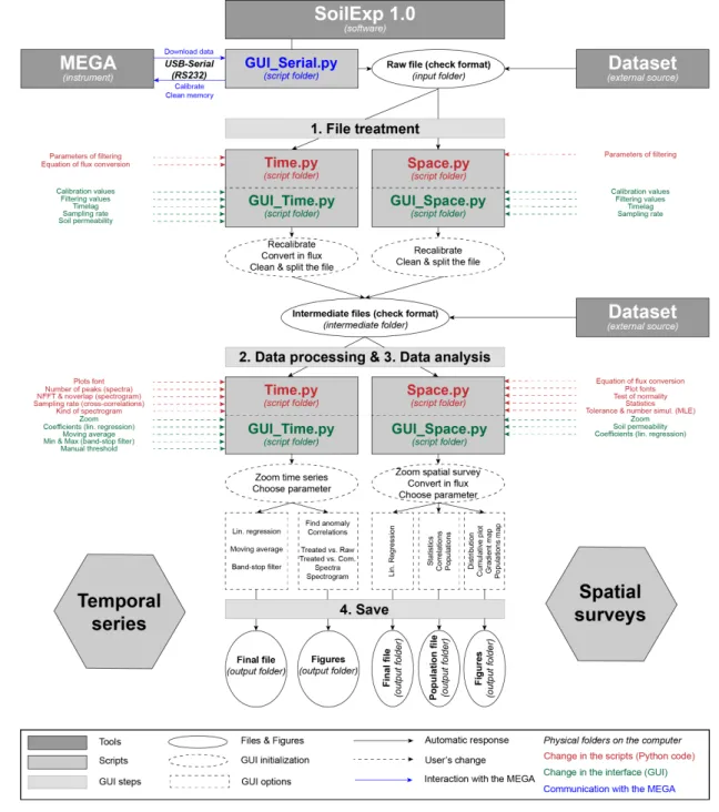
The SoilExp software: An open-source Graphical User Interface (GUI) for post-processing spatial and temporal soil surveys
Texte intégral
Figure

Documents relatifs
In this paper a new control system called Franklin is presented to be used with CNC machines in general and 3-D printers specifically. It was developed while exploring
In or- der to support this kind of development method, software is required throughout the user interface development life cycle in order to create, edit, check models that
To make the collection process of the hard metrics more efficient, we developed a web service to gather quantifiable FOSS project information from Open Hub and GitHub
L’archive ouverte pluridisciplinaire HAL, est destinée au dépôt et à la diffusion de documents scientifiques de niveau recherche, publiés ou non,. The Practice of Free and Open
The Free and Open Source Software (f/oss) model is a philosophy and method- ology characterized by development and production practices that support ac- cess to the sources
The focus of this review is to describe the potential interplay between oxygen, iron and sulfide in the oral ecosystem, especially in the subgingival plaque,
de déposition est déterminé par les facteurs source, trarrsport et aussi par les ri principales conditions de la surf'ace du substrat.. Chapitre I : Propriétés
maximus est corrélée positivement à la concentration en matière particulaire en suspension (Szostek et al. A notre connaissance, aucune étude ne permet de déinir si : i)
