Adaptive filtering for global interference cancellation and real-time recovery of evoked brain activity: a Monte Carlo simulation study

Adaptive filtering for global interference

cancellation and real-time recovery of evoked

brain activity: a Monte Carlo simulation study

The MIT Faculty has made this article openly available.

Please share

how this access benefits you. Your story matters.

Citation

Zhang, Quan, Emery N. Brown, and Gary E. Strangman. “Adaptive

Filtering for Global Interference Cancellation and Real-Time

Recovery of Evoked Brain Activity: a Monte Carlo Simulation Study.”

Journal of Biomedical Optics 12, no. 4 (2007): 044014. © 2007

Society of Photo-Optical Instrumentation Engineers

As Published

http://dx.doi.org/10.1117/1.2754714

Publisher

SPIE

Version

Final published version

Citable link

http://hdl.handle.net/1721.1/87658

Terms of Use

Article is made available in accordance with the publisher's

policy and may be subject to US copyright law. Please refer to the

publisher's site for terms of use.

Adaptive filtering for global interference cancellation

and real-time recovery of evoked brain activity:

a Monte Carlo simulation study

Quan Zhang

Harvard Medical School Massachusetts General Hospital Neural Systems Group

13th Street, Building 149, Room 2651 Charlestown, Massachusetts 02129

Emery N. Brown

Department of Anesthesia and Critical Care Massachusetts General Hospital

Department of Brain and Cognitive Sciences Harvard-MIT Division of Health Science

and Technology

Massachusetts Institute of Technology

Gary E. Strangman

Harvard Medical School Massachusetts General Hospital Neural Systems Group

13th Street, Building 149, Room 2651 Charlestown, Massachusetts 02129

Abstract. The sensitivity of near-infrared spectroscopy 共NIRS兲 to

evoked brain activity is reduced by physiological interference in at least two locations: 1. the superficial scalp and skull layers, and 2. in brain tissue itself. These interferences are generally termed as “global interferences” or “systemic interferences,” and arise from cardiac ac-tivity, respiration, and other homeostatic processes. We present a novel method for global interference reduction and real-time recovery of evoked brain activity, based on the combination of a multisepara-tion probe configuramultisepara-tion and adaptive filtering. Monte Carlo simula-tions demonstrate that this method can be effective in reducing the global interference and recovering otherwise obscured evoked brain activity. We also demonstrate that the physiological interference in the superficial layers is the major component of global interference. Thus, a measurement of superficial layer hemodynamics共e.g., using a short source-detector separation兲 makes a good reference in adaptive inter-ference cancellation. The adaptive-filtering-based algorithm is shown to be resistant to errors in source-detector position information as well as to errors in the differential pathlength factor共DPF兲. The technique can be performed in real time, an important feature required for ap-plications such as brain activity localization, biofeedback, and poten-tial neuroprosthetic devices.© 2007 Society of Photo-Optical Instrumentation

Engi-neers. 关DOI: 10.1117/1.2754714兴

Keywords: near-infrared spectroscopy; brain; neuronal; hemodynamics; Monte Carlo; adaptive filter; interference; cancellation.

Paper 06351R received Dec. 2, 2006; revised manuscript received Apr. 18, 2007; accepted for publication Apr. 20, 2007; published online Jul. 16, 2007.

1 Introduction

Over the past 15 years, near-infrared spectroscopy共NIRS兲 and diffuse optical imaging共DOI兲 have been used to detect hemo-dynamic or neuronal changes associated with functional brain activity in a variety of experimental paradigms.1–16Compared with existing functional methods共e.g., fMRI, PET, EEG, and MEG兲, the advantages of NIRS and DOI for studying brain function include good temporal resolution, measurement of both oxygenated hemoglobin 共O₂Hb兲 and deoxygenated he-moglobin 共HHb兲, nonionizing radiation, portability, and low cost.4,6Disadvantages include modest spatial resolution, lim-ited penetration depth, potential sensitivity to hair absorption and motion artifacts, and global interference共also called sys-temic physiological interference兲.

Global interference can arise from at least two spatial sources: 1. in the superficial layers共such as scalp and skull兲, and 2. inside brain, due to factors such as heart activity, res-piration, and spontaneous low frequency oscillations关i.e., low frequency oscillations 共LFOs兲 and very low frequency

oscil-lations 共VLFOs兲兴.17–21 In empirical studies of brain function using NIRS and DOI, the amount of global interference varies from subject to subject and from time to time. In some cases, the amount of interference is small and evoked brain activity can be seen in the raw measurement; other times the amount of interference is too large for the evoked brain activity to be detected without signal processing.18 Several methods have been explored for the removal of global interference and im-provement of evoked brain activity measurements. Low pass filtering is the most common and straightforward, as it is highly effective in removing cardiac oscillations.22,23 How-ever, for physiological variations such as respiration, LFOs, and VLFOs, there is a significant overlap between their fre-quency spectra and that of the hemodynamic response to brain activity. Frequency-based removal of these interferences can therefore result in large distortion and inaccurate timing for the recovered brain activity signal. Other methods for improv-ing the contrast-to-noise ratio共CNR, mean signal during task performance minus mean signal during baseline, divided by the noise兲 for NIRS-based brain function measurements in-clude adaptive average waveform subtraction,24 direct sub-traction of a “nonactivated” NIRS waveform,22 state space 1083-3668/2007/12共4兲/044014/12/$25.00 © 2007 SPIE

Address all correspondence to Quan Zhang, Harvard Medical School, Neural Systems Group, MGH-13th St, Building 149, Rm 2651, Charlestown, MA 02129 United States of America; Tel:共617兲 724–5550; Fax: 共617兲 726–4078; E-mail: qzhang@nmr.mgh.harvard.edu

estimation,25–27and principal components analysis.28

Recently, Morren et al. adopted the technique of adaptive filtering to remove cardiac oscillations, using signals acquired from pulse oximetry as a reference.29Adaptive filtering has been widely used in interference cancellations,30,31 and has great potential in the removal of global interferences and re-covery of evoked brain activity detection, as demonstrated in EEG and MRI studies.32The advantage of adaptive filtering includes its capability of following the signal’s nonstationary changes and its simple implementation with low computa-tional overhead. Since biomedical signals are generally non-stationary and real-time features are desired for most NIRS applications, adaptive filtering has the potential to be a good fit for NIRS applications. Morren et al. showed that this method effectively removes the cardiac-related signal varia-tion in the optical measurements. However, in the applicavaria-tion of evoked brain activity detection, global interference in-cludes not only cardiac oscillations but also other physiologi-cal variations such as vasomotor waves and respiration, which are not represented by pulse oximetry signals. Moreover, pulse oximetry is often measured from fingers or toes, far from the head, and acquires measurements at different wave-lengths. Thus, this reference signal is less representative of the NIRS signal observed during head measurements and hence is not optimal for reducing head/brain-based interferences.

In evoked brain activity detection, a good reference mea-surement used in adaptive interference cancellation should be highly correlated to the global interference. Ideally, it mea-sures directly the interference while avoiding any sampling of the evoked response. Previously, researchers have used opti-cal measurements with short interoptode distances for moni-toring superficial layer hemodynamics.17,20 For example, McCormick et al. have attempted to measure interference from superficial layers using short source-detector separation to correct cerebral oxygen delivery monitoring.20No detailed algorithm for interference correction was presented in their publication, and the superficial layer interference measure-ment was used simply to visually compare measuremeasure-ments from far source-detector separations rather than for interfer-ence correction. The methodology we developed combines a multiseparation probe for data collection and adaptive filter-ing for signal processfilter-ing, and it can be used in conjunction with the existing methods such as low pass filtering. This method has low computational requirements, and hence can be implemented in real time, an important feature needed for potential applications for real-time brain function localization procedures, biofeedback, and potential neuroprosthetic devices.

2 Multidistance Optode Configuration and

Adaptive Filtering Algorithm to Remove

Global Interference

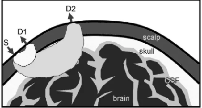
According to a photon transport theory,33photons propagating through a highly scattering tissue travel along a zig-zag path before they are detected. The collective photon propagation follows a roughly banana-shaped pattern 共formulated by three-point Green’s function34,35兲 when reflection geometry is used, as in most applications of NIRS in the measurement of neuronal activity 共see Fig. 1兲. With appropriate source and detector placement, we can make one channel primarily

sen-sitive to the shallow layer hemodynamic changes共S-D1, with close separation of source and detector; Fig. 1兲 and another channel sensitive to hemodynamic changes, both in the shal-low layer 共unavoidably兲 and on the cerebral cortex 共S-D2, with far separation of source and detector兲. In adaptive inter-ference cancellation, measurements from S-D2 can be used as a target signal channel, and with measurements from S-D1 used as reference channel. This process is equivalent to as-suming a linear mapping between the shallow layer hemody-namics, acquired from S-D1, and the global interference in the target measurement from S-D2. Optimized cancellation is then achieved by a point-to-point optimization of this linear mapping. This cancellation, and hence the improvement in CNR, is maintained even when hemodynamic changes in the superficial layer are nonstationary, so long as the changes are relatively slow compared to the adaptive filter convergence rate.

Our study used the continuous wave共CW兲 NIRS method, where two wavelengths共690 and 830 nm兲 of light are shone into the head, detected at the scalp’s surface, and then are converted to relative changes in the concentration of deoxy-hemoglobin 共HHb兲 and oxyhemoglobin 共O2Hb兲 using the modified Beer-Lambert law.5,34,36,37 First we calculate the changes in the absorption coefficient by:

⌬␮a共␭兲 = ln

I0共␭兲

I共␭兲/共DPF · d兲, 共1兲

where I₀is the baseline light intensity, or the light intensity at the initial time, and I is the time-dependent light intensity.

DPF is the differential pathlength factor, a constant that

ac-counts for the scattering properties of tissue, and d is the separation between the source and the detector. After solving the equations ⌬␮a共␭1兲 = ln共10兲␧HHb共␭1兲⌬关HHb兴 + ln共10兲␧O₂Hb共␭1兲⌬关O2Hb兴 共2兲 ⌬␮a共␭2兲 = ln共10兲␧HHb共␭2兲⌬关HHb兴 + ln共10兲␧_O 2Hb共␭2兲⌬关O2Hb兴,

we obtain the concentration of ⌬关HHb兴, the variation of deoxygenated hemoglobin, and ⌬关O2Hb兴, the variation of Fig. 1 Multisource-detector separation approach. Superficial layer he-modynamics acquired from S-D1 will be used to estimate the global interference presented in the target measurement from S-D2, which is then canceled using adaptive filtering.

oxygenated hemoglobin, as a function of time. The␧’s are the specific extinction coefficients of deoxygenated and oxygen-ated hemoglobin at different wavelengths. Water content is assumed to be stable, thus is not shown in Eq.共2兲.

An adaptive filter with a finite impulse response共FIR兲 and transversal structure 共tapped delay line兲 is used in our global interference cancellation.38The filter output signal eiis given

by:

e_i= y_i−

兺

k=0 M

␻k,ixi−k. 共3兲

Here the⌬关HHb兴 共or ⌬关O₂Hb兴兲 acquired from far source-detector separations共S-D2 in Fig. 1兲, which contains evoked brain hemodynamic changes, is used as the target measure-ment共the signal channel兲, denoted by yi. The subscript i is the

index of the time point. The⌬关HHb兴 共or ⌬关O₂Hb兴兲 acquired from short source-detector separations共S-D1 in Fig. 1兲 is used as reference measurement共the reference channel兲, denoted by

xi. M represents the order of the filter and the␻kare the filter

coefficients, where k is the coefficient index. Since the coef-ficients are adjusted by the filter output ei on a sample by

sample basis, we use␻_k,ito denote the k’th coefficient at time

i. Coefficients were updated via the Widrow-Hoff least mean

square 共LMS兲 algorithm.39This algorithm is simple and fast, features needed for real-time applications, especially for ap-plications such as diffuse optical imaging where hundreds of channels would have to be processed together in real time. The LMS algorithm for optimization is:

␻k,i=␻k,i−1+ 2␮eixi−k, 共4兲

where the constant ␮ is a step size, which controls the con-vergence rate of the algorithm.

The processing steps proceed as follows. First, we calcu-late the⌬关HHb兴 共or ⌬关O₂Hb兴兲 time series for both close and far source-detector separations, xiand yi, respectively. These

time series become the inputs to the adaptive filter. The adap-tive filter converts xi, the hemodynamic and oxygenation

variation associated with the superficial layers, to an estimate of the global interferences embedded in yi. Finally, this

esti-mate is then subtracted from the original time series. The transfer function of the adaptive filter is optimized dynami-cally, via LMS关Eq. 共4兲兴, to ensure the best quality of cancel-lation and account for variations of the living tissue. To expe-dite the convergence of the LMS algorithm, we can normalize the two time series xiand yi, so that both have standard

de-viations close to one. In real application on human subjects, such normalization could be achieved by collecting共e.g.兲 rela-tively short共30 to 60 sec兲 pretest recordings prior to running the main experiment. Pretests will also allow pretraining of the adaptive filter to acquire good initial FIR filter coefficients.

The performance of the filter is controlled by the order of the FIR filter M and the step size used in updating the FIR nodes ␮. Note that if M= 1, the adaptive filter becomes a straight subtraction:

ei= yi−␻0xi, 共5兲

with␻₀as a scaling factor. A previous study by Franceschini et al. demonstrated a CNR improvement of approximately 20% by subtracting manually selected “nonactivated” pixels from other pixels when imaging brain activities,22 which is equivalent to assigning␻0a fixed value of 1. Instead of using a nonactivated channel共which presupposes knowledge of ac-tivation in the face of noisy data兲, as shown in Eq. 共5兲, we use short source-detector separation measurements to estimate global interference and a scaling factor to adaptively adjust the quantitative value. Here,␻0can be adjusted using Eq.共4兲, or in some cases be estimated and updated dynamically ac-cording to the instant variation amplitudes of the xi and yi

time series. For example,␻₀= std共yi兲/std共xi兲, where std

indi-cates estimation of standard deviation using current or short-term data. Since different tissue areas may have different blood concentrations 共and different variations in amplitude兲, in many cases by assigning␻₀a fixed value of 1, we may not be able to remove all interference. Adaptive filtering depends more on the relative variation rather than their absolute mag-nitude, thus by performing adaptive filtering we expect the result to be further improved.

3 Monte Carlo Simulation Study of Evoked

Brain Activity Recovery

3.1 Simulation Design

To assess the performance of our methodology, we developed a Monte Carlo simulation of head tissue, using layered struc-tures to simulate scalp, skull, CSF, white matter, and gray matter, respectively. One light source location with two wave-lengths, 690 and 830 nm, and two detectors were located on the surface of the medium to collect reflectance data. Simu-lated cardiac oscillations and respiration are used as sources of global variations, and they present in all layers. A proto-typical hemodynamic response in the gray matter layer was introduced via synchronous reduction of关HHb兴 and increased 关O2Hb兴. The “stimulation” paradigm was a common block-design paradigm composed of alternating blocks of15 sec of rest and 15 sec of stimulation, for a total of 200 sec. Data were collected at a sampling rate of 10 Hz, and scattering properties of tissue throughout the simulation were assumed to be stable. The adaptive filtering used measurements from S-D1 as reference to acquire an estimate of global interfer-ence 共1.5-cm separation兲 and measurements from S-D2 as a target dataset共4.5-cm separation兲 to acquire evoked hemody-namic response after removal of global interference. By com-paring the raw measurements from S-D2, recovered evoked response and the true evoked response, we evaluated the fil-ter’s ability to remove unrelated physiological variations from the hemodynamic response.

3.2 Simulating Global Interference and Evoked Functional Brain Hemodynamics

Generally, multiple Monte Carlo simulations have to be per-formed to acquire the simulated time series. However, using the tMCimg Monte Carlo program 共implemented in C兲,40,41 pathlengths through the simulated tissue are recorded for each photon detected. So for different time points where only ab-sorption changes, the result can be calculated without

rerun-ning the whole simulation. We launched 100,000,000 photons from the source for the simulated data collection at each time point. As shown in Fig. 2, the size of the simulated tissue is 150⫻100⫻50 mm3_{. The thickness and scattering properties} selected for each layer can be found in the first column of Table 1. Because the source and detectors are in the middle of the simulated tissue surface, the boundary effect was ignored. The index of refraction mismatch was also ignored in this study共both tissue and air were given a refraction index of 1兲. The hemodynamic changes in the scalp, skull, CSF, and gray and white layers were simulated as a combination of cardiac fluctuation c共t兲, respiratory fluctuations r共t兲, and func-tional hemodynamic responses v共t兲. In a real experiment,

there would be a certain amount of uncorrelated changes in the superficial layers compared with deep layers. For ex-ample, the skin may sweat, which will only produce varia-tions in the scalp layer. To simulate this phenomenon, we also introduced a slow varying random time series g共t兲 in the scalp layer response. In summary:

f_HHb1 共t兲 = HHb₀1+ g共t兲关A_HHb1 c共t兲 + B_HHb1 r共t兲 + C_HHb1 v共t兲兴, 共6兲 f_O 2Hb 1 _{共t兲 = O} 2Hb0 1_{+ g共t兲关A} O₂Hb 1 _{c共t兲 + B} O₂Hb 1 _{r共t兲 + C} O₂Hb 1 _v共t兲兴, 共7兲 f_HHb2,3,4,5共t兲 = HHb₀2,3,4,5+ A_HHb2,3,4,5c共t兲 + B_HHb2,3,4,5r共t兲 + C_HHb2,3,4,5v共t兲, 共8兲 fO₂Hb 2,3,4,5_{共t兲 = O} 2Hb0 2,3,4,5 + AO₂Hb 2,3,4,5 c共t兲 + BO₂Hb 2,3,4,5 r共t兲 + CO₂Hb 2,3,4,5 v共t兲, 共9兲 where f_HHb1 共t兲, f_O 2Hb 1 _{共t兲, f} HHb 2,3,4,5_{共t兲, and f} O2Hb 2,3,4,5_{共t兲 represent the} concentration of deoxygenated and oxygenated hemoglobin in each layer as a function of time, with the superscripts 1 to 5 indicating the layer index for scalp, skull, CSF, and gray and white matters, respectively. HHb0 and O2Hb0 represent the average or baseline concentrations. The coefficients A, B, and

C with layer index as superscript and HHb or O₂Hb as sub-script are the hemodynamic variation amplitude control pa-rameters. They are used to adjust the magnitude of variations of deoxygenated and oxygenated hemoglobin concentrations in each layer due to cardiac pulsation, respiration, and evoked brain response. The values of the previously described param-eters, including the baseline concentration and the variation amplitude control parameters A, B, C for deoxygenated and oxygenated hemoglobin in each layer, can be found in Table 1. Since this study focuses on signal and hemodynamic varia-tions, the constant absorption from water and other back-ground chromophores is not considered. The parameters used are based on Choi et al.42and others,34,43–45together with our own human subject data.

The cardiac and respiratory oscillations c共t兲 and r共t兲 were both simulated as amplitude- and frequency-varying sinu-soidal oscillations:

c共t兲 = Mheartsin共2␲fheartt兲, 共10兲 Fig. 2 Geometry of the Monte Carlo simulation for removal of global

interferences and recovery of evoked brain activity.

Table 1 Hemodynamic parameters used in the Monte Carlo simulation.

Head layers Blood content Baseline concentration 共␮M兲 respirationA共␮M兲, B共␮M兲, heartbeat C共␮M兲, evoked response Scalp, 7 mm 共␮s⬘=10 cm−1兲 O2Hb 39 2 1.1 0 HHb 16 0.13 0.074 0 Skull, 7 mm, 共␮s⬘=12 cm−1兲 O2Hb 39 2 1.2 0 HHb 16 0.13 0.078 0 CSF, 1 mm共␮s⬘=0.1 cm−1兲 O2Hb 11.7 0.2 0.12 0 HHb 4.8 0.01 0.006 0 Gray matter, 3 mm 共␮s⬘=5 cm−1兲 O2Hb 56 2 1.2 15 HHb 20 0.13 0.076 −4 White matter, 33 mm 共␮s⬘=7 cm−1兲 O2Hb 56 2 1.1 0 HHb 20 0.13 0.072 0

r共t兲 = Mrespsin共2␲frespt兲, 共11兲 where M_heart, f_heart, M_resp, and f_respare all random variables, and were generated by low pass filtered Gaussian white noise 共with offset added兲. The average value and standard deviation of the previous variables and the bandwidth of the low pass filter 共fourth order, Butterworth兲 used to filter the Gaussian white noise are listed in Table 2. These values were chosen based on our human subject data.

The evoked hemodynamic responsev共t兲 was defined as the

convolution of the stimulation paradigm s共t兲, 关s共t兲=0 for rest and 1 for stimulation兴 and a prototypical hemodynamic im-pulse response h共t兲46: s共t兲 =

再

冉

冊

冉

冊

Independent scalp variation g共t兲 is also generated by bi-ased and low pass filtered Gaussian white noise; its related information can be found in Table 2.

The hemoglobin concentration changes at each layer were converted to reduced absorption coefficients using a linear transform with specific extinction coefficients at 690 and 830 nm. Monte Carlo simulations were performed using the prior parameters共about 15 h of compute time on a Gateway 450 laptop兲, and the simulated fluence rate for a 2000 point time series共200 sec of data at a sampling rate of 10 Hz兲 was calculated without rerunning the Monte Carlo for each time point 共the calculation for one entire time series took about 32 h in Matlab兲. Noise was then added to the acquired simu-lated optical measurements. Simusimu-lated electronic noise was generated by low pass filtered white noise to 3 Hz, with a standard deviation of 1/100 standard deviation caused by res-piration and heart beat.

3.3 Determining Differential Pathlength Factor and Sensitivity Correction Factor

Differential pathlength factor is a correction to the source-detector separation, which is used to estimate the actual

path-length a photon propagates through the medium.33 Usually,

DPFs are defined for homogeneous medium; for the

hetero-geneous medium used in the Monte Carlo simulation, we tried two ways to determine the DPF. First, we used CW light in the Monte Carlo simulation and determined the DPFs by:

DPF = lnU0

U

⌬␮ad

, 共15兲

where U₀ is the baseline measurement acquired from Monte Carlo, U is the measurement with a small and known pertur-bation⌬␮ain all layers, and d is the source-detector

separa-tion. In the second method, we used radio frequency 共RF兲 modulated light 共70 MHz兲. In our simulation, the average phase delay of the optical measurement at each detector is acquired, and this phase delay is proportional to the average photon propagation length, thus we can determined the DPF using the phase delay via

DPF = ␸c

2␲f␭d, 共16兲

where ␸ is the phase delay after the diffuse photon density wave 共DPDW兲 propagates through the medium, acquired from the Monte Carlo simulation; c is the speed of light; f is the modulation frequency共e.g., 70 MHz, the result is not sen-sitive to modulation frequency changes兲; ␭ is the index of refraction; and d is the source-detector separation. The results are presented in Table 3.

DPFs were variable, depending on separation and wave-length. The difference between the results from these two methods is less than 2%. Part of this error may be because the photon propagation pattern 共banana pattern兲 for RF and CW are different. Since we are using CW illumination in the simu-lation, we applied the results from the CW method to our further data analysis.

When comparing the recovered brain hemodynamic changes with the true evoked hemodynamic response v共t兲,

since surface measurements are more sensitive to superficial layers and there is a partial volume effect 共i.e., in the tissue probed by the light, the blood concentration changes in the gray layer part are “averaged” to the whole volume兲, we can-not compare the quantitative filtered results directly with the expected values. To examine the quantitative performance of our methodology, we calculated the sensitivity correction scaling factor by introducing a known perturbation into the blood content of the gray matter layer only and then calculat-ing the blood content changes uscalculat-ing the surface measurements Table 2 Simulation parameters for amplitude and frequency of

inter-ference oscillations.

Parameters

Baseline

共average兲 value Standarddeviation

Bandwidth of the low pass filter共Hz兲

Mheart共a.u.兲 1 0.32 0.8

fheart共Hz兲 1.1 0.003 0.2

Mresp共a.u.兲 1 0.18 0.2

fresp共Hz兲 0.18 0.002 0.1

g共t兲 共a.u.兲 1 0.1 0.01

Table 3 Calculated DPFs using CW and RF methods.

690 nm 830 nm Methods S-D1 共1.5 cm兲 共4.5 cm兲S-D2 共1.5 cm兲S-D1 共4.5 cm兲S-D2 CW method 5.4 7.0 5.1 6.6 RF method 5.5 7.1 5.2 6.7

and the modified Beer-Lambert law共MBLL兲. The sensitivity correction factor is defined as the ratio of true blood content change to measured blood volume change. For our simulation, this sensitivity correction factor is calculated to be about 27.

3.4 Simulated Optical Measurements

Figure 3 shows the raw simulated optical measurement at 690 nm and its power density spectrum, acquired from the 1.5- and 4.5-cm source-detector separations. The simulated measurements qualitatively match human subject data.47The gray bars indicate blocks of evoked stimulation. As from the raw time series and from the power density spectrum, neither the simulated measurements from S-D1 nor from S-D2 show any obvious evoked response, because the signal variation is dominated by global interference, i.e., respiration and heartbeat.

3.5 Adaptive-Filtering-Based Removal of Global Interference and Recovery of Simulated Hemodynamic Response

After the simulated optical measurements are acquired, the data analysis described in Sec. 2.1 is applied. For the filtering parameters, considering both convergence speed and filter sta-bility, we chose␮= 0.0001 and we use M = 100, about twice as large as the average period of the respiration fluctuation. To speed up the convergence, we prenormalized the target and

the reference datasets by dividing by their estimated standard deviation, so that both time series have a standard deviation of approximately 1. After the adaptive filtering, the quantitative values of the filtered results were recovered by multiplying back the standard deviation. The initial guess of the adaptive filter weights was关1 0 ... 0兴, in other words we assume that the shape of the global interference and the S-D1 measure-ments are identical at the beginning of the adaptive filtering. 关O2Hb兴 and 关HHb兴 were filtered separately and are presented in Figs. 4 and 5, respectively. In these figures, we show both raw time series of calculated blood concentration 共the first column兲 and their block averaged results 共the second column兲. For the block average results, we average from 5 sec prior through25 sec after the onset of each simulated stimulation. The gray bars indicate the period of active stimulation.

In Fig. 4, where the O2Hb result is presented, the target dataset for adaptive filtering is the calculated 关O2Hb兴 from S-D2 with 4.5-cm source-detector separation 关Figs. 4共a兲 and 4共b兲兴, and the reference dataset is the calculated关O₂Hb兴 from S-D1 with 1.5-cm source-detector separation 关Figs. 4共c兲 and 4共d兲兴. In theory, the target dataset should contain the evoked hemodynamic response; however, neither its raw time series 关Fig. 4共a兲兴 nor its block average 关Fig. 4共b兲兴 show visible sig-nal change correlated with the stimulation paradigm. In fact, its similarity 共both in the raw time series and the block aver-Fig. 3 Simulated optical measurements at 690 nm from S-D1 and S-D2共a兲 and 共c兲, together with their power density spectrum 共b兲 and 共d兲.

ages兲 to the reference dataset 关Figs. 4共c兲 and 4共d兲兴 indicates that it is dominated by global interferences.

After adaptive filtering, as seen from the filtered result 关Figs. 4共g兲 and 4共h兲兴, approximately 80% of the signal varia-tion has been removed. This is another indicavaria-tion that the signal variations in the target dataset are predominantly global interferences that correlate well with the superficial layer re-sponses. After we multiplied the sensitivity correction factor back into the filtered result, we compared it with the real evoked brain hemodynamic changes in the gray matter layer. The comparison can be seen in Figs. 4共i兲 and 4共j兲, with the solid line as the filtered result recovered after sensitivity cor-rection, and the dashed line as the true evoked brain response used in the simulation. Although obvious interferences still remain, the contrast-to-noise ratio is dramatically improved for evoked hemodynamic response detection. We also see, quantitatively, good agreement between the filtered result 共af-ter sensitivity correction兲 and the true value. Cardiac and res-piration variations were significantly reduced, even without the application of any bandpass filtering. The CNR of the evoked response can be further improved by block averaging 关Fig. 4共j兲兴, since the global variations are not temporally cor-related 共due to the random factors in the frequency and am-plitude of heartbeat and respiration兲, and can be canceled and thus suppressed significantly by block averaging.

Comparing the recovered evoked hemodynamics 关solid line in the block average results, Fig. 4共j兲兴 with the real un-derlying hemodynamics 关dashed line in the block average re-sult, Fig. 4共j兲兴, we noticed several types of errors. 1. Residual interference: the recovered evoked response is not as smooth as the real hemodynamics, due to the leftover global interfer-ence after filtering. 2. Quantitative error: the amplitude of the recovered evoked response is about 85% of the real value. 3. Timing error or phase lag: the rise and fall of the evoked response has a small amount of time delay compared with the real hemodynamic response. Residual interference is ex-pected, as no technique will completely remove truly random interference. In our adaptive filtering, the error may be be-cause the random factor g共t兲 in superficial layers reduced the correlation between the global interference in the superficial layers and the global interference in the brain layers. In addi-tion, the convergence of the LMS algorithm is relatively slow, and the results may improve when another adaptive filtering algorithm with faster convergence is used.

We also compared the adaptive filtering result with a tra-ditional low pass filtering result.关O₂Hb兴 acquired from S-D2 关Fig. 4共a兲兴 was low pass filtered with an eighth-order Butter-worth filter with 0.5-Hz bandwidth, and the result is shown in Figs. 4共e兲 and 4共f兲. From Fig. 4共e兲, we can see that this low Fig. 4 Adaptive filtering to remove global interference and to recover evoked brain activity.共a兲 target O2Hb measurements from S-D2 with 4.5-cm

source-detector separation and共b兲 its block averaged result. 共c兲 and 共d兲 Reference measurements from S-D1 with 1.5-cm source-detector separa-tion.共e兲 and 共f兲 Low pass filtering result for the target measurements. 共g兲 and 共h兲 Adaptive filtering result for the target measurement. 共i兲 and 共j兲 Adaptive filtering result with sensitivity correction 共solid line兲, together with the true evoked brain activity 共dashed line兲 used for quantitative comparison and evaluation of the performance of the adaptive filtering method.

pass filter effectively removes the cardiac oscillations; how-ever, systemic variations due to respiration remain. After block average, seen in Fig. 4共f兲, the systemic interference was further suppressed; however, it is still too large for the evoked brain activity to be detected. Comparing Fig. 4共f兲 with the final adaptive filtering block averaged result 关Figs. 4共h兲 and 4共j兲兴, we can see that adaptive filtering removes the global interference and recovers the evoked brain activity much more effectively.

In Fig. 5, we show the equivalent of Fig. 4 but for关HHb兴. The evoked response is visible, although noisy, after block averaging without adaptive filtering 关Fig. 5共b兲兴. This is be-cause the amount of global interference in关HHb兴 is relatively small. After adaptive filtering, the global interference is sig-nificantly removed, CNR increased, and the evoked response can be clearly seen关Figs. 5共g兲 and 5共h兲兴. The performance of adaptive filtering for interference removal and evoked brain activity detection can be further demonstrated with sensitivity correction关Figs. 5共i兲 and 5共j兲兴. As for O2Hb, we can see there are still interferences left; however, cardiac and respiration variations were significantly reduced, again without bandpass filtering. The quantitative value of the functional blood con-centration change was recovered to about 80% of the ex-pected value. When comparing adaptive filtering result with

the low pass filtering result shown in Figs. 5共e兲 and 5共f兲 using an eighth-order Butterworth filter with 0.5-Hz bandwidth, we can see that this low pass filter again effectively removes the cardiac oscillations; however, systemic variations due to res-piration remain. After block averaging关Fig. 5共f兲兴, the evoked brain activity can be clearly seen, and systemic interference was further suppressed; however, the residuals are still quite obvious. In comparison, the final adaptive filtering block av-eraged result 关Figs. 5共h兲 and 5共j兲兴 has much less residual in-terferences and improved CNR.

Both 关O₂Hb兴 and 关HHb兴 demonstrated approximately 20% quantitative error after adaptive filtering 关Figs. 4共j兲 and 5共j兲兴. We hypothesized that there was a small sensitivity to brain tissue at a 1.5-cm separation, and the evoked brain ac-tivity detected by the reference channel was removed from the signal channel after adaptive filtering, resulting in reduced filtered results. This hypothesis was supported by the fact that when we re-ran the simulations using a reference separation of1.0 cm in place of 1.5 cm, we were able to recover 95% of the expected value of functional blood concentration change 共result not shown兲. Generally, using a reference that is partly correlated with the expected hemodynamic response will re-sult in a loss in quantitative accuracy when filtering. Optimi-zation of the selection of reference channels for the best fil-Fig. 5 Adaptive filtering to remove global interference and to recover evoked brain activity.共a兲 Target HHb measurements from S-D2 with 4.5-cm source-detector separation and共b兲 its block averaged result. 共c兲 and 共d兲 Reference HHb measurements from S-D1 with 1.5-cm source-detector separation.共e兲 and 共f兲 Low pass filtering result for the target measurements. 共g兲 and 共h兲 Adaptive filtering result for the target measurement. 共i兲 and 共j兲 Adaptive filtering result with sensitivity correction 共solid line兲, together with the true evoked brain activity 共dashed line兲 used for quantitative comparison and evaluation of the performance of the adaptive filtering method.

tering performance will be studied and reported in the future. Together, our Monte Carlo simulations show that, in prin-ciple, our methodology significantly removes global interfer-ence and improves the CNR in evoked brain activity detec-tion.

4 Resistance to Positional Errors

and Differential Pathlength Factor Errors

Errors in the location of optical sources and detectors and in the assumed DPFs are two major error sources in NIRS using CW measurements and MBLL. Both affect the quantitative values of the result significantly, but less on the relative varia-tions or the shape of the关O₂Hb兴 and 关HHb兴 time series. Since this adaptive-filtering-based method uses mostly the shape of the time series rather than the quantitative values of the time series, it is resistant to the errors in source and detector posi-tion measurements or in DPFs. One example demonstrating this method’s resistance to DPF error is shown in Fig. 6. The optical measurements are the same as described in Sec. 3.2; however, when calculating the 关O2Hb兴 and 关HHb兴 time se-ries, the DPFs used for S-D1 and S-D2 are 4.3 and 5.6 at 690 nm, and 3.6 and 4.6 at 830 nm共i.e., introduction of 25% error兲. From the result we see that the quantitative values of 关O2Hb兴 and 关HHb兴 changed; however, the global interfer-ences are still effectively removed and evoked responses suc-cessfully detected, although the quantitative values of the re-covered evoked response changed due to DPF error. Generally speaking, when DPFs are underestimated, the re-constructed quantitative values will be overestimated and vice versa. This effect, however, will be systematic throughout an experiment, such that all measurements will be over- or un-derestimated in a similar way, preserving comparability in terms of relative change.

An example demonstrating our method’s resistance to po-sitional error is shown in Fig. 7. In this test, we introduced random positional error 共generated in Matlab using the func-tion “randn,” with standard deviafunc-tion of5 mm兲. Again, global interferences are effectively removed and evoked responses are still successfully detected, although the quantitative values

of the recovered evoked response changed due to source and detector positional error. Generally, when source-detector separation estimates are smaller than the real separations, the calculated blood concentration will be larger than the results using the correct separations, and vice versa.

5 Comparison of Shallow Layer Hemodynamics

and Global Interference

The performance of the adaptive-filtering-based removal of the global interference depends on how well the global inter-ference共in the target measurement from S-D2兲 and the refer-ence measurement 共from S-D1兲 are correlated. In principle, global interference in the target dataset comes from all layers, since respiration, heart beat, and related hemodynamics could exist in all tissue types. Our reference measurement, however, is predominantly sensitive to shallow layer hemodynamics, and hence changes there may differ from those in deeper lay-ers. Two major reasons conspire to make the reference mea-surements and the global interference in the target measure-ments correlate well: 1. sensitivity dominance of the superficial layer, and 2. physiological connection between su-perficial and deeper layers.

5.1 Sensitivity Preeminence of Superficial Layers

First, superficial layer variation is the predominant component in the total global interference in the noninvasive surface measurement. According to photon transport theory, even for measurements with large source-detector separation like S-D2, the surface measurements are more sensitive to super-ficial layer changes.34,35 Although the total global interfer-ences consist of superficial layer hemodynamic variations and deep-layer hemodynamic variations, the superficial layer he-modynamic variation comprises a much larger portion of the total global interferences. Hence, a measurement of the super-ficial layer hemodynamics is a very good choice for a refer-ence measurement in a noninvasive reflectance probe geometry.

Our Monte Carlo simulation allows us to look at the total global interference and its components共i.e., from superficial Fig. 6 Adaptive filtering results using inaccurate DPFs共25% error兲.

layers and from cerebral layers兲 separately. This is done as follows. To acquire total systemic interference, we performed simulation with the same parameters as those we described in Sec. 3.2, except that there is no evoked hemodynamic re-sponse added to the gray layer. Then, to acquire the compo-nent of global interference from superficial layers, we per-formed simulation with the respiration and cardiac hemodynamics restricted to scalp and skull layers only. Fi-nally, to acquire the component of global interference from deep layers, we restricted the respiration and cardiac to gray and white matters layers only. Again, those simulation time series are calculated based on recorded photon pathlength in-formation without rerunning individual Monte Carlos at each time point. Simulated optical measurements were acquired from S-D2 with 4.5-cm source-detector separation, and then blood content was calculated using MBLL.

The关O2Hb兴 result is shown in Fig. 8, where the solid line represents the total global interference in O2Hb, acquired when respiration and cardiac hemodynamics exists in all lay-ers; the dotted line represents the global variations from scalp and skull; and the dashed line represents the variations from deep brain layers. As Fig. 8 shows, the total global interfer-ence and its components look very similar. Quantitatively, the interference from scalp and skull is the major component, and it is about 80% of the total global interference, which is ap-proximately the same proportion of the signal removed during adaptive filtering. This decomposition of total global interfer-ence clearly demonstrates the sensitivity preemininterfer-ence of su-perficial layers for optical measurements with source-detector separation of4.5 cm in our simulation.

5.2 Physiological Connection between Superficial and Deep Layers

Shallow and deep layer hemodynamics should be correlated due to their close physiological connections. In a human sub-ject, the heart, blood vessels, and lungs are the sources of the global pressure-induced oscillations, and the carotid artery is the common gateway for both scalp and skull共shallow兲 and brain 共deep兲 hemodynamic oscillations. Thus, correlation is expected, even if the enclosed state of the tissue inside the

skull alters the shape of the oscillatory waveforms. In our simulation, the hemodynamic variations in the superficial lay-ers 共scalp, skull兲 and deep layers 共gray, white matter兲 were generated using linear combinations of respiration and cardiac waveforms. The factors that differ between the superficial and deep layers in our simulations included: 1. g共t兲 to simulate independent scalp processes such as sweating, 2. different relative weight on respiration and cardiac wave, which changes the final waveforms, 3. different scattering for each layer, and 4. electronic noise. Although we have added these factors to make the superficial and deep-layer hemodynamics different, when correlating shallow-layer variation time series and deep variation time series, the correlation coefficient is 0.9986.

Due to these two reasons, the measurement of the superfi-cial layer hemodynamics using short source-detector separa-tion provides a good estimate of the global interference in the target measurement for evoked brain activity detection, and enables good adaptive filtering performance. This conclusion appears to hold up in human subject experiments, which will be reported separately.47

6 Real-Time Implementation

of the Methodology

The LMS adaptive filtering algorithm we discussed is particu-larly suited to real-time implementation. We have imple-mented the algorithm in C + + and tested it共Intel Pentium M processor, 2000 MHz, 400-MHz external bus兲, and it is ca-pable of processing 833 K data points共64 bit data type兲 per second with adaptive filtering 共M =100兲. For a typical DOI imaging system with 50 sources, 50 detectors 共2500 chan-nels兲, and 100-Hz sampling rate, the time required to process all data collected in1 sec with adaptive filtering is 0.3 sec, or 30% of the total time 共70% can be used for data acquisition and other processing兲. Therefore, a real-time removal of glo-bal interference and recovery of evoked brain activity is prac-tical on even modestly current computer hardware, an impor-tant feature required for applications such as brain activity localization, biofeedback, and potential neuroprosthetic devices.

7 Discussion

Using Monte Carlo simulation, we demonstrated that one should be able to combine a multiseparation probe configura-tion with adaptive filtering to dramatically reduce global in-terference and improve the CNR in evoked brain activity de-tection. We further demonstrated that superficial layer interference is the major component of the total global inter-ference, making superficial layer hemodynamics a particularly good estimate for the total global interference. An added ad-vantage of our method is its suitability for real-time use.

In previous studies,23,34,48 we utilized simple, traditional signal conditioning methods共high and low pass filtering兲. The implicit assumption was that the overlying layers, even if they do interfere with the brain measurement, do not correlate with the stimulation protocol and hence can be reduced or elimi-nated by block averaging or statistical methods. Across stud-ies, however, we have consistently observed notable intersub-ject variability in 1. the robustness of evoked responses and 2. the magnitude of nonevoked variability 共especially cardiac Fig. 8 Total global interference and its components. Solid line

共la-beled 1兲 is the total global interference in the 关O2Hb兴 from S-D2 in the

simulation; dotted line共labeled 2兲 is the interference from superficial scalp and skull layers; and dashed line共labeled 3兲 is the interference from deep layers of gray and white matters.

and respiratory oscillations兲. Based on our findings here— particularly the observation that approximately 80% of our raw signal is removed during filtering—we suggest that the robustness of noninvasively recorded evoked brain responses may, at least in some cases, be much more severely affected by interference from overlying tissue layers than previously assumed. Preliminary application of this technique to human data supports this suggestion.

While we tried to make the simulation as realistic as we could, it is not possible to include every potential physiologi-cal variable. In the Monte Carlo simulation work, we chose to include respiration and cardiac oscillations, with respiration being representative of lower frequency oscillations 共and in-deed we selected a relatively low frequency for respiration of 0.18 Hz兲. In the human subject case report, the major inter-ferences were found to be Mayer waves and cardiac, and it was demonstrated that they were also effectively removed by adaptive filtering. In principle, with appropriate reference sig-nal and adaptive filter design, adaptive filtering helps to re-move interferences with different types.

In this study we performed adaptive filtering after convert-ing raw signal to blood content. Roughly speakconvert-ing, the raw optical signal is an exponential function of the blood concen-tration or absorption coefficient; the total measurement is a product of contributions from global interference and evoked brain hemodynamics. Linear adaptive filtering does not work well in this case, since here the output signal is total signal minus 共not divided by兲 estimated interference. Put another way, there is a nonlinear operation 共logarithm兲 between raw intensity and ⌬关O₂Hb兴 and ⌬关HHb兴, and nonlinear opera-tions cannot be transposed to get the same answer. However, after the raw optical measurements are converted to absorp-tion coefficients 共i.e., after taking the logarithm兲, then there should be minimal difference switching the linear procedures of blood conversion 共using the absorption coefficient兲 and adaptive filtering. Since the result will be presented as hemo-dynamics共blood concentration variations兲 at the end, the DPF error cannot be avoided. Conceptually it is relatively easier to explain the physiology and discuss the interference from O2Hb and HHb separately. In addition, in many of our human subject studies we found that the interference in O2Hb and HHb are different. While information about O2Hb and HHb are merged in the raw signals at each wavelength, converting the raw signal to blood components first gives us the flexibil-ity of choosing which blood species we will perform the adap-tive filtering on to get the greatest benefit.

Three limitations of the method need to be mentioned. First, in this study the stimulation paradigm and the global interference were uncorrelated. In some experiments, how-ever, the evoked brain activity and the global interference may be correlated to some degree. For example, tasks requiring exertion may increase respiration and heart rates in concert with task performance, thereby making the global interference and brain activity coupled. How well our adaptive filtering will work for this scenario is still under investigation. Gener-ally, error will occur if the reference time series and the signal to detect are correlated, and this error depends on the magni-tude of correlated components in the two time series. Second, good performance of our method depends on measurements from S-D1 with short source-detector separation correlating well with the global interference in measurements from S-D2.

In our simulation the head is assumed to be layered homog-enous, while those layers in an actual human head can be very heterogeneous, e.g., due to the heterogeneous distribution of large blood vessels. We are susceptible to independent optical changes around the location of D1, or movement of D1 inde-pendent of D2. In principle, adaptive filtering effectively re-moves only interferences that are contained both in the target measurement and in the reference channel; any independent changes or noise in the reference measurement can be added 共with inverted sign兲 into the target measurement by the sub-traction step in the filtering process. Thus, the reference mea-surement needs to be as free from artifact as possible. One possible solution might be to collect more than one short source-detector separation reference measurement and to combine or select these references as needed. Third, as com-pared with the true evoked hemodynamic response, the re-sponse recovered via adaptive filtering still has leftover inter-ferences, as well as quantitative error and phase distortion. The focus of this study is to preliminarily demonstrate the methodology, and solutions to the previously mentioned limi-tations are under investigation.

Overall, the combination of a multidistance probe and adaptive filtering appears quite promising for removing a ma-jor source of error in NIRS for evoked brain activity detec-tion. Such filtering may be particularly useful in studies of the optical fast signal,2,16,29where signals are small and lowpass filtering removes the signal of interest along with the noise. In depth discussion about the optimization of the adaptive filter parameters and comparison of different adaptive filter struc-tures will be reported in the future. In our tests, we have observed that the best parameters 共M and␮兲 in the adaptive filter are relatively robust and do not vary substantially from case to case. By optimizing the probe configuration and algo-rithm, for example choosing the best source-detector separa-tions for the reference measurement and target measurement, or using adaptive filtering algorithms with faster convergence 共e.g., normalized LMS, recursive least squares, adaptive RLS兲, we may be able to further improve the performance of this methodology.

Acknowledgments

This work was supported by the National Institutes of Health 共K25-NS46554 and R21-EB02416兲. We would also like to thank the PMI laboratory at Massachusetts General Hospital for the Monte Carlo simulation code 共available at http:// www.nmr.mgh.harvard.edu/PMI/resources.htm兲, and thank Margaret Duff for her help in preparing the manuscript.

References

1. J. Steinbrink, A. Villringer, F. Kempf, D. Haux, S. Boden, and H. Obrig, “Illuminating the BOLD signal: combined fMRI-fNIRS stud-ies,” Magn. Reson. Imaging 24共4兲, 495–505 共2006兲.

2. J. Steinbrink, F. C. D. Kempf, A. Villringer, and H. Obrig, “The fast optical signal-robust or elusive when non-invasively measured in the human adult?,” Neuroimage 26共4兲, 996–1008 共2005兲.

3. T. J. Huppert, R. D. Hoge, S. G. Diamond, M. A. Franceschini, and D. A. Boas, “A temporal comparison of BOLD, ASL, and NIRS hemodynamic responses to motor stimuli in adult humans,”

Neuroim-age 29共2兲, 368–382 共2006兲.

4. E. Gratton, V. Toronov, U. Wolf, M. Wolf, and A. Webb, “Measure-ment of brain activity by near-infrared light,” J. Biomed. Opt. 10, 011008共2005兲.

5. A. Villringer and B. Chance, “Non-invasive optical spectroscopy and imaging of human brain function,” Trends Neurosci. 20共10兲, 435–442

共1997兲.

6. G. Strangman, D. A. Boas, and J. P. Sutton, “Noninvasive brain im-aging using near infrared light,” Biol. Psychiatry 52, 679–693共2002兲. 7. C. Hirth, H. Obrig, J. Valdueza, U. Dimagl, and A. Villringer, “Si-multaneous assessment of cerebral oxygenation and hemodynamics during a motor task—a combined near infrared and transcranial Dop-pler sonography study,” Oxygen Transport Tissue 18, pp. 461–469, Plenum Press, New York共1997兲.

8. A. Villringer, J. Planck, C. Hock, L. Schleinkofer, and U. Dirnagl, “Near-infrared spectroscopy 共Nirs兲—a new tool to study hemodynamic-changes during activation of brain-function in human adults,” Neurosci. Lett. 154共1-2兲, 101–104 共1993兲.

9. W. N. Colier, V. Quaresima, B. Oeseburg, and M. Ferrari, “Human motor-cortex oxygenation changes induced by cyclic coupled move-ments of hand and foot,” Exp. Brain Res. 129, 457–461共1999兲. 10. V. Toronov, M. A. Franceschini, M. Filiaci, S. Fantini, M. Wolf, A.

Michalos, and E. Gratton, “Near-infrared study of fluctuations in ce-rebral hemodynamics during rest and motor stimulation: temporal analysis and spatial mapping,” Med. Phys. 27共4兲, 801–815 共2000兲. 11. M. A. Franceschini, V. Toronov, M. E. Filiaci, E. Gratton, and S.

Fantini, “On-line optical imaging of the human brain with 160-ms temporal resolution,” Opt. Express 6共3兲, 49–57 共2000兲.

12. K. Matsuo, N. Kato, and T. Kato, “Decreased cerebral haemodynamic response to cognitive and physiological tasks in mood disorders as shown by near-infrared spectroscopy,” Psychol. Med. 32共6兲, 1029– 1037共2002兲.

13. J. Ruben, R. Wenzel, H. Obrig, K. Villringer, J. Bernarding, C. Hirth, H. Heekeren, U. Dirnagl, and A. Villringer, “Haemoglobin oxygen-ation changes during visual stimuloxygen-ation in the occipital cortex,”

Oxy-gen Transport Tissue 19 428, 181–187共1997兲.

14. K. Sakatani, S. Chen, W. Lichty, H. Zuo, and Y. P. Wang, “Cerebral blood oxygenation changes induced by auditory stimulation in new-born infants measured by near infrared spectroscopy,” Early Hum.

Dev. 55共3兲, 229–236 共1999兲.

15. B. Chance, Z. Zhuang, C. Unah, C. Alter, and L. Lipton, “Cognition-activated low-frequency modulation of light-absorption in human brain,” Proc. Natl. Acad. Sci. U.S.A. 90共8兲, 3770–3774 共1993兲. 16. M. A. Franceschini and D. A. Boas, “Noninvasive measurement of

neuronal activity with near-infrared optical imaging,” Neuroimage 21共1兲, 372–386 共2004兲.

17. H. Obrig, M. Neufang, R. Wenzel, M. Kohl, J. Steinbrink, K. Ein-haupl, and A. Villringer, “Spontaneous low frequency oscillations of cerebral hemodynamics and metabolism in human adults,”

Neuroim-age 12共6兲, 623–639 共2000兲.

18. D. A. Boas, A. M. Dale, and M. A. Franceschini, “Diffuse optical imaging of brain activation: approaches to optimizing sensitivity, im-age, resolution, and accuracy,” Neuroimage 23, S275-S288共2004兲. 19. M. Kohl-Bareis, H. Obrig, K. Steinbrink, K. Malak, K. Uludag, and

A. Villringer, “Noninvasive monitoring of cerebral blood flow by a dye bolus method: separation of brain from skin and skull signals,” J.

Biomed. Opt. 7共3兲, 464–470 共2002兲.

20. P. W. McCormick, M. Stewart, M. G. Goetting, M. Dujovny, G. Lewis, and J. I. Ausman, “Noninvasive cerebral optical spectroscopy for monitoring cerebral oxygen delivery and hemodynamics,” Crit.

Care Med. 19共1兲, 89–97 共1991兲.

21. P. W. McCormick, M. Stewart, G. Lewis, M. Dujovny, and J. I. Ausman, “Intracerebral penetration of infrared light,” J. Neurosurg. 76共2兲, 315–318 共1992兲.

22. M. A. Franceschini, S. Fantini, J. H. Thomspon, J. P. Culver, and D. A. Boas, “Hemodynamic evoked response of the sensorimotor cortex measured noninvasively with near-infrared optical imaging,”

Psycho-physiology 40共4兲, 548–560 共2003兲.

23. G. Jasdzewski, G. Strangman, J. Wagner, K. K. Kwong, R. A. Poldrack, and D. A. Boas, “Differences in the hemodynamic response to event-related motor and visual paradigms as measured by near-infrared spectroscopy,” Neuroimage 20共1兲, 479–488 共2003兲. 24. G. Gratton and P. M. Corballis, “Removing the heart from the brain:

compensation for the pulse artifact in the photon migration signal,”

Psychophysiology 32共3兲, 292–299 共1995兲.

25. V. Kolehmainen, S. Prince, S. R. Arridge, and J. P. Kaipio, “State-estimation approach to the nonstationary optical tomography prob-lem,” J. Opt. Soc. Am. A 20共5兲, 876–889 共2003兲.

26. S. Prince, V. Kolehmainen, J. P. Kaipio, M. A. Franceschini, D. Boas, and S. R. Arridge, “Time-series estimation of biological factors in optical diffusion tomography,” Phys. Med. Biol. 48共11兲, 1491–1504

共2003兲.

27. S. G. Diamond, T. J. Huppert, V. Kolehmainen, M. A. Franceschini, J. P. Kaipio, S. R. Arridge, and D. A. Boas, “Dynamic physiological modeling for functional diffuse optical tomography,” Neuroimage 30共1兲, 88–101 共2006兲.

28. Y. H. Zhang, D. H. Brooks, M. A. Franceschini, and D. A. Boas, “Eigenvector-based spatial filtering for reduction of physiological in-terference in diffuse optical imaging,” J. Biomed. Opt. 10共1兲, 011014 共2005兲.

29. G. Morren, U. Wolf, P. Lemmerling, M. Wolf, J. H. Choi, E. Gratton, L. De Lathauwer, and S. Van Huffel, “Detection of fast neuronal signals in the motor cortex from functional near infrared spectros-copy measurements using independent component analysis,” Med.

Biol. Eng. Comput. 42共1兲, 92–99 共2004兲.

30. S. Selvan and R. Srinivasan, “Processing of abdominal fetal electrocardiogram—a review,” IETE Tech. Rev. 17共6兲, 369–384 共2000兲.

31. H. A. Mansy and R. H. Sandler, “Bowel sound signal enhancement using adaptive filtering—separating heart sounds from gastrointesti-nal acoustic phenomena,” IEEE Eng. Med. Biol. Mag. 16共6兲, 105–117 共1997兲.

32. G. Bonmassar, P. L. Purdon, I. P. Jaaskelainen, K. Chiappa, V. Solo, E. N. Brown, and J. W. Belliveau, “Motion and ballistocardiogram artifact removal for interleaved recording of EEG and EPs during MRI,” Neuroimage 16共4兲, 1127–1141 共2002兲.

33. D. T. Delpy, M. Cope, P. Vanderzee, S. Arridge, S. Wray, and J. Wyatt, “Estimation of optical pathlength through tissue from direct time of flight measurement,” Phys. Med. Biol. 33共12兲, 1433–1442 共1988兲.

34. G. Strangman, M. A. Franceschini, and D. A. Boas, “Factors affect-ing the accuracy of near-infrared spectroscopy concentration calcula-tions for focal changes in oxygenation parameters,” Neuroimage 18共4兲, 865–879 共2003兲.

35. M. A. O’Leary, “Imaging with diffuse photon density waves,” Ph.D. Thesis, Univ. Pennsylvania, Philadelphia共1996兲.

36. D. A. Boas, T. Gaudette, G. Strangman, X. Cheng, J. J. A. Marota, and J. B. Mandeville, “The accuracy of near infrared spectroscopy and imaging during focal changes in cerebral hemodynamics,”

Neu-roimage 13, 76–90共2001兲.

37. D. T. Delpy, M. Cope, P. van der Zee, S. Arridge, S. Wray, and J. Wyatt, “Estimation of optical pathlength through tissue from direct time of flight measurement,” Phys. Med. Biol. 33, 1433–1442共1988兲. 38. J. L. Semmlow, Biosignal and Biomedical Image Processing,

Matlab-Based Applications, Marcel Dekker, Inc., New York共2004兲.

39. S. Haykin, Adaptive Filter Theory. Prentice-Hall, Upper Saddle River, NJ共2001兲.

40. D. A. Boas, J. P. Culver, J. J. Stott, and A. K. Dunn, “Three dimen-sional Monte Carlo code for photon migration through complex het-erogeneous media including the adult human head,” Opt. Express 10共3兲, 159–170 共2002兲.

41. See http://www.nmr.mgh.harvard.edu/DOT/resources/tmcimg/ index.htm.

42. J. Choi et al., “Noninvasive determination of the optical properties of adult brain: near-infrared spectroscopy approach,” J. Biomed. Opt. 9, 221–229共2004兲.

43. S. Kohri, Y. Hoshi, M. Tamura, C. Kato, Y. Kuge, and N. Tamaki, “Quantitative evaluation of the relative contribution ratio of cerebral tissue to near-infrared signals in the adult human head: a preliminary study,” Physiol. Meas 23共2兲, 301–312 共2002兲.

44. T. S. Leung, C. E. Elwell, and D. T. Delpy, “Estimation of cerebral oxy- and deoxy-haemoglobin concentration changes in a layered adult head model using near-infrared spectroscopy and multivariate statistical analysis,” Phys. Med. Biol. 50共24兲, 5783-5798 共2005兲. 45. E. Okada and D. T. Delpy, “Near-infrared light propagation in an

adult head model. I. Modeling of low-level scattering in the cere-brospinal fluid layer,” Appl. Opt. 42共16兲, 2906–2914 共2003兲. 46. M. S. Cohen, “Real-time functional magnetic resonance imaging,”

Methods 25共2兲, 201–220 共2001兲.

47. Q. Zhang, E. N. Brown, and G. E. Strangman, “Adaptive filtering to remove global interference in evoked brain activity detection: a hu-man subject case study,” J. Biomed. Opt.,共in press兲.

48. G. Strangman, J. C. Culver, J. H. Thompson, and D. B. Boas, “A quantitative comparison of simultaneous BOLD fMRI and NIRS re-cordings during functional brain activation,” Neuroimage 17, 719– 731共2002兲.