HAL Id: hal-02827169
https://hal.inrae.fr/hal-02827169
Submitted on 7 Jun 2020
HAL is a multi-disciplinary open access
archive for the deposit and dissemination of sci-entific research documents, whether they are pub-lished or not. The documents may come from teaching and research institutions in France or abroad, or from public or private research centers.
L’archive ouverte pluridisciplinaire HAL, est destinée au dépôt et à la diffusion de documents scientifiques de niveau recherche, publiés ou non, émanant des établissements d’enseignement et de recherche français ou étrangers, des laboratoires publics ou privés.
To cite this version:
Jean-Marc Boussard, Marie-Gabrielle Piketty. Risk in the commodity chain: The sugar example. [Other] 2001, 30 p. �hal-02827169�
Jean-Marc BOUSSARD* and Marie-Gabrielle PIKETTY**
23 November 2001
Contributed paper to the congress of the International Association of Agricultural Economists, Berlin, August 2000.
Revised version
* INRA, Paris, France
Address : 45 bis, avenue de la Belle Gabrielle, 94736 Nogent-sur-Marne Cedex
** CIRAD, Paris, France
Address : 45 bis, avenue de la Belle Gabrielle, 94736 Nogent-sur-Marne Cedex [email protected]
Risk in the commodity chain :
The sugar example.
Jean-Marc BOUSSARD and Marie-Gabrielle PIKETTY
ABSTRACT
A sectoral model of the world sugar industry is presented. Results suggest that sugar prices are naturally chaotic. As a consequence, and contrary to the conventional creed, liberalisation, instead of damping fluctuations out, is likely to increase them. But since decision makers are risk averse, and restrain production when faced with uncertain prices, the average price level without is significantly lower than with liberalisation, thus jeopardising the benefits of a more efficient use of resources due to comparative advantage. The policy implication is that care should be taken not to create undesired situations for the right purpose of a better division of labour between nations.
According to common wisdom, sugar is one of these commodity for which the desirability of liberalization is not questionable. There are three good reasons for that :
i – In Europe and Japan, as well as in many other countries, sugar producers are relatively wealthy farmers, for whom the classical “poor farmer argument” –it would be necessary to support incomes by providing high price guarantees because farmers are poor, and that something must be done for helping the poor- obviously does not apply 1/. On the contrary, the many restrictions to sugar production and exchange implemented in these countries are harmful to consumers, who could otherwise enjoy much cheaper sweetened foods.
ii – By constraining the benefits from trade and comparative advantage, these policies introduce inefficiency into the whole world sugar system. In particular because of the low price of manpower and because sugar cane is probably more efficient than the sugar beet as a solar energy converter, production costs are far smaller in developing than in developed countries. The latter should therefore cease to produce inefficiently, and let poor developing countries enjoy the benefit of the few advantages they can claim without discussion, for the ultimate satisfaction of consumers everywhere.
iii – World sugar prices are volatile. Indeed, they reach peaks in volatility, when compared with other volatile commodities (BOURGES, 1998). This volatility is detrimental for the whole
1/ Notice it nevertheless may apply to developing countries : sugar producers in India or Pakistan are not the wealthier farmers… And they are a lot of people !
system, as shown as early as 1944 by an author such as WAUGH(1944)2/. It should be therefore removed as far as possible. Now, it turns out that this extreme price volatility must be related with another characteristic of the sugar commodity chain. Only a small part of the production and consumption is presently exchanged through markets. The bulk of production is shielded off from price fluctuations. The world sugar market is typically regarded as a residual market where national economies dump their surpluses that arise because production, due to yield variations, exceed even strict quotas. It is tempting to jump from relation to causality, and infer from the above observations that volatility is the consequence of market narrowness. Under this line of reasoning, liberalization would widens the base for price formation, and stabilize market by the virtue of the law of large number, because droughts or floods rarely occur at the same time in different continents. Trade would therefore play the role of a costless insurance, for the greater advantage of both producer and consumer.
In what follows, we shall not discuss the first two reasons for sugar market liberalization. They are fully justified, and no economist can seriously challenge them. In particular, it is not true to say that taking advantage of the low cost of manpower in developing countries would not bring any other benefits than the ruin of the wealthy developed country farmers : the latter have better to do than inefficient sugar production. They should reorient their efforts in these activities where they have a true comparative advantage, thus widening the joint production possibility set, just as would a technical progress do. Yet, there exist serious problems with the third reason, which does not seem to be so strong as it may appear at first glance. It is indeed the theme which will be developed here that, because markets are probably not capable of solving the volatility problem, and because the losses due to this circumstance are enormous, it may very well happen that the losses associated with point i and ii be only a least evil –an evil which would be replaced by something much worse if corrected by standard liberalization, and withdrawal of all state regulation.
The only possible demonstration of this type of assertion consists in building up a model which could be run “with” and “without” liberalization, in such a way as to compare both situations one with another. Many such models have been built up in the past 3/ -most of
them more or less similar in their conclusion, matching the three reasons for liberalization given above. This unanimity in the outcome is not too surprising since these models are also unanimous in the premises. Under classical free trade assumptions, with no expectation errors, producers equating expected and marginal cost, and utility maximizing consumers, it is well known that any restriction to trade implies a loss of welfare. It would be surprising that any model built along this line would yield a different conclusion. But is this framework fully
2/ Eventually, the pertinacity of the
WAUGH’s conclusion regarding the consequences of volatility for different categories of agents, such as consumers or producers has been questioned. The controversy lasted for years, and produced a large body of literature. Yet, nobody, as far as we know, never argued that volatility could be socially beneficial.
3/ For instance,
WILLIAM and ISHAM (1999) quote 19 of them recently published –and they are probably not
justified ? The contention here is that it is not, mainly because there exist expectation errors, and because risk averse producers will be “variance elastic” as much as “price elastic”.
This is not new : for instance BOUSSARD (1996) developed a theoretical modified cobweb model, with constant (and constantly false !) mean price expectation, and a producer behavior driven by risk aversion : instead of maximizing expected profit, the producer is assumed to maximize a Markowitz utility function, that is a linear combination of expected mean profit and expected variance of profit. The expected variance of price, itself, is “naïve” –the squared difference between this year and last year price. Under this assumption, the price and quantity series of the cobweb model is shown to be chaotic (in the mathematical sense of the word) over a certain fractal subset of the model parameters subspace. As a consequence, the volatility of the price series is not “random exogenous” but “built-in endogenous”, and its general properties are quite different from those of a normal “white noise” series, although it may look similar at first inspection. Especially, while the sum of two white noises is a new white noise, the volatility of which is smaller than the sum of the volatilities of the original series, two chaotic motions forced to “trade” one with each other may just synchronize, yielding a new chaotic series with about the same characteristics as the original ones 4/ (ALLIGOOD et al., 1997 p. ).
The BOUSSARD’s paper just summarized was only theoretical. Apart for demonstrating the possibility of endogenous fluctuation in a simple dynamic supply and demand system, its main virtue was its ability to be run on a spread sheet. But could such phenomena be reproduced into a larger, “real life” model of a commodity such as sugar, embedded into reality, just as the many models of the sugar market alluded to above demonstrate the possibility of expanding the text book model of supply and demand into computer programs aiming at providing numerical estimates of the benefits of liberalization ? The exercise reported here is an attempt in this direction, with the ambition of providing an estimate of the magnitude of the “loss” associated with “free trade” under these circumstances.
I – Model description
It is extremely similar to most other models of the sugar industry, especially the famous Australian ABARE model (HAFI et al. , 1993; SHEAL et al.1999 ), which was widely
used by international organization to demonstrate the magnitude of the benefit to be expected from a liberalization of the world sugar market. Especially, it borrows many features and elasticities to the latter. By comparison with the ABARE model, the main originalities are as
follows :
1°) No statistical estimation of parameters
There is no attempt for obtaining new statistical estimates of the model parameters. When such estimates may be considered as reliable, as for instance in the case of demand elasticities, we made use of results already published, essentially those provided by ABARE.
When technical data were available, especially in the production modules, we made use of them, for two reasons. First, in general, any well known technical relationship, independent of the model at hand, is always better than any statistical estimate, valid only for the particular statistical framework used to get it. Second, if all observed series are actually chaotic, and cannot be converted into white noise by a suitable transformation, it is well known that standard statistical procedure are of no much use for getting reliable estimates5. The econometrics of chaotic series, on the other hand, is still in infancy. Thus, it seemed that in such case, guess estimates of unknown parameters were at least not worse than apparently more rigorous statistical analysis –and they were much easier to implement.
2°) Systematic introduction of Markowitz utility functions
The maximization of profit, in all segments of the model where it may take place, is systematically replaced by a Markowitz utility function 6/ . The Markowitz utility function of a random income z is given by:
(4) where U is utility, z a random income, with expected mean and expected variance , and A an absolute risk aversion coefficient.
As a consequence, maximising U subject to :
(5) implies the following first order conditions :
(6) which opens the way to ill-shaped supply curves, as noticed a long time ago by JUST and ZILBERMAN (1986). It has to be noticed from the above equations that the main difference between a production with quota at guaranteed prices and a production at market price lies in the fact that in the second case, production may decrease even when mean expected price are high, and, for instance, higher than guaranteed price, if price volatility is too important. One virtue of market stabilisation policies is to avoid the dampening effect of price volatility on supply.
In effect, in the model reported here, this kind of utility function is assumed to be maximised by :
5 See for instance TONG (1990), and many others.
6/ The Markowitz utility function, widely used in finance, has been severely criticized by decision theory
analysts. At best, it stands as a clumsy approximation of the VON NEUMAN / MORGENSTERN expected utility theory,
not even satisfying the basic axioms of stochastic dominance. Yet, it is easy to use, and convenient in first approximation. At least, it is certainly better to make use of such an imperfect instrument than to neglect the problem entirely.
i – farmers, when deciding each year how much future contract they will pass with sugar processing factories 7/.
ii – Sugar processing factories, when they decide how much future contract to buy from farmers and sugar refineries when they decide how much raw sugar will be processed into white sugar.
iii – Sugar processing factories, when, acting as stockholder, they decide how much sugar to sell out of their stocks, on the spot market.
iv – Refineries and sugar processing factories, when they decide to invest in new capacities from their past benefits.
In each case, the A absolute risk aversion coefficient is computed as the inverse of the average wealth of the corresponding decision maker, thus implicitly assuming an approximately constant relative risk aversion coefficient 8/. In this way, a major characteristic
of the heterogeneity of decision makers is taken into account, since the heterogeneity in wealth can be considered as a summary of all kinds of heterogeneity.
3°) Introduction of a complex expectation scheme
An implication of the above line of reasoning, however, is the necessity of a complex expectation scheme. For if utility functions depend on prices mean and variance, then, expectations must also pertain on both moments of the probability function. In principle, the two should be completely parallel. If, for instance, the expectation pertaining to mean is a weighed sum of past observations, then the variance should be same weighed sum of square deviations from the mean estimate. But why should weights be the same ?
In addition, any observed regularity is likely to permit high benefits. It is notorious that many traders and market operators are trying to detect cycles in price series. This would imply that any clue of cycle in the data should be interpreted as a periodic mean, and a variance reduced accordingly. But such a reasoning opens way to even more arbitrariness and
ad hoc hypothesis generation.
An escape from this dilemma is provided by “rational expectations”, after the famous idea by MUTH. Yet, rational expectations are also a minefield 9/, unless one accept the idea that
equilibrium prices, by definition, are the only possible definition of rational expectations. Current casual observation shows that this idea does not reflect reality, while reflection suggests that the word, if it means anything, means that available information is rationally processed by decision makers. Then, the problem is simply displaced, for nobody knows which information is available, and what is a rational way of processing it. Yet, the correct answer to the above question is a matter of facts. One cannot be satisfied with the classical
7/ In effect, farmers pass a sort of future contracts with processing plants, the latter offering to buy the whole
production at current price at harvest time. Farmers decision is then which sugar density of production (i.e., tons of sugar per ha of total agricultural area) do they have to promise. Processing plant’s decision is which agricultural area to prospect. More details are provided below.
8/ It is well known that A, the absolute risk aversion coefficient, and α, the relative risk aversion coefficient, are
related by A = α/w, where w is the wealth of the decision maker. See PRATT(1964).
9/ In this respect, the remark by
LUCKE (1992) that rational expectations, in the case of sugar, are logically impossible, must be taken into consideration.
standard hypothesis according to which “rational decision makers expect equilibrium”, unless this affirmation is confirmed by empirical data and surveys. Unfortunately, very few references report any valuable information in this respect. It is therefore the probably most important contribution of the present exercise to conclude that expectation formation is a crucial point in any recursive model of this type and that future researches in this field are badly needed.
In the meantime, the results presented below were obtained with what we experienced as the scheme providing the “best” results – “best” being judged in terms of the similarity between “real” and “modelled” time series, as discussed below. In this way, the model presented here relies on some sort of extension of the notion of "maximum likelihood". In effect, these "best" results were obtained with a variance expectation computed from a two years moving average expectation scheme . In the case of stockholders, this “guess” about mean and variance is subject to an important correction. Since the total world existing stock is public and well known guesses are modified by the level of this stock : mean expected price is decreased when stock are too high and conversely.
4°) Processing plants and stockpiling consideration
Just as in the ABARE model, stockpiling plays a major role here. However, we tried to
have a better description of this important function through two modelling innovations.
The first is that, instead of a yearly elementary time unit, ours is monthly, thus allowing to picture the seasonal character of the generated price series. Of course, harvesting is yearly, although the year is not the same in the southern hemisphere and in the north. But consumers consume each month, and stockholders have to proceed time arbitrage. Each month processing-stockpiling plants must make a choice between selling, or keeping the current level of stock. The stock is increased regularly at harvested period.
The second is the introduction of risk as it has been mentioned before. Indeed, nobody would keep any stock unless there is some expectation of profit. And given this expected profit (value of sales, minus costs), nobody would sell it unless there is some risk of loss. Here, the risk is instrumental in regulating the instantaneous supply and demand. The current spot price is the adjustment variable which determines the level of profit necessary to convince stockholders to keep the equilibrium quantity in stock, given their risk aversions 10.
The expected profit from carrying over a stock St from time t to time t + 1 is given by :
(7) where is the net of cost expected price for t + 1, and Pt is the spot equilibrium price of
time t. The variance of expected profit is , where is the expected variance associated with the expected mean price . The current spot price pt is then computed in
such a way as to clear current month sugar market, assuming each stockholder is maximising , according to risk aversion A.
What is very important in this treatment of stockpiling is that, contrary to some conventional wisdom, this activity may not always reduce price volatility. Indeed, because of imperfect
10/ Notice this line of reasoning is borrowed from N
expectations, traders may sell their stocks at period with low price or keep them whereas prices finally decrease in the next period. Moreover, higher price volatility tends to increase large immediate selling which may by itself reinforce price fluctuations.
5°) Other non linearity
Another point which deserves attention in setting up a model of this type is the agricultural production function. As in many such models, we assumed here a very simple reaction from farmers. They just maximise their utilities from a CES function of sugar and “others” productions 11/. Our results imply therefore that nothing change in the “other”
productions conditions while sugar price means and variances are continuously changing. All this is classical, and hardly needs comments.
There is nevertheless in the present model a peculiarity which is tied with a specificity of sugar, may explain some of our results, and deserves explanations. As noticed above, sugar must be processed very quickly after harvest. This means that sugar producers must not be located too far from the processing plant. But how far is too far ?
To provide an endogenous answer to this question, it has been assumed that producers were deciding not simply “a sugar production”, but rather a “geographical density of sugar production” – a sugar quantity per square kilometre of the total surface of a region. Then, processing plants have to collect this sugar over the area of a disc. It is easy to show (BOUSSARD, 1987, p.215 ) that in this case, the cost of collection per kg of sugar is growing as the square root of the radius of the disc, thus implying a somewhat strange marginal cost. Thus, if the profit of sugar processing is large, it may be profitable to increase the capacity of production, and build a new plan in a virgin area 12/.
These two features (marginal cost of one plant growing as the power ½ of the radius of the contemplated surface and possibility of increasing capacity by reinvesting benefits) are present in our model, and play a role in the generation of irregular price series. Similarly, the capacity of refineries can also be increased, through the reinvesting of profits 13/ However,
again, risk plays a role in limiting such investments, since the quantity of money invested in a plant is determined by the relative expected profits and variance of the investment, as compared with profit and variances of alternative uses of money, the latter being exogenous.
11/ An assumption also present in the
ABARE model, through the introduction of "price of competing crops".
Here, the price of competing crop is held constant, and only the CES substitutability coefficient matters. These
two ways of representing the same phenomenon are substitutable...
12/ As a consequence, any sugar factory enjoys a “monopsony power” over supplier farmers. It is tempting to
exaggerate the consequences of this situation. If the benefits from exerting this monopsony power were so large, then why should not competitors try their chance ? A possible explanation could be sought for in the industry Malthusianism. Without neglecting such a possibility, it must be noticed that we provide here a strong technical reason for the perenity of a situation which would certainly not have lasted for so long a time if driven only by “sheer force”.
13/ The introduction of a “ratchet effect” in the refinery capacity is the main innovation of the model by W
ILLIAM AND ISHAM (1999). They explain that uncertainty is unimportant in the sugar industry, while the dynamics of investment in production capacity is. This is exactly what we say here, except that expectations are also
important, and that “uncertainty” as defined by these authors –that is, the risk deriving from climate and other
Finally, the behaviour of final consumers is represented by a banal constant elasticity demand curve of the individual consumer, calibrated from the condition that present consumption per head conform with present observed behaviours at present prices. In addition, the number of consumers in each country is determined by demographic considerations. In the absence of any other estimates, the elasticity's determined by ABARE
were used throughout.
II – A taste of results
The model described above is thus made of a large quantity of submodels, each of which being relatively simple and “classical” in its spirit. Yet, but the main unknown lies in the behaviour of the whole, when constrained by necessity of clearing markets. Two kinds of simulations can be envisaged with such an instrument :
1°) First it is possible to run the model using the present policies constraints (mainly
EC, US and ACP production or imports quotas, imports taxes) in order to see if the generated
price series would resemble to what can be observed in reality 14/. Notice that no random
exogenous shocks are added in the model, thus making any observed irregularity purely endogenous 15/.
2°) It is also possible to compare the consequences of alternative policies, in order to see whether one is “better” – according to some social judgement criteria – than others.
Both type of experiment have been made with the present model.
Validation
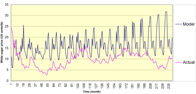
Figure 1 and table 1 show a comparison of “actual” and “modeled” white sugar world price over 240 month. “Actual” stands for the last 240 month available sugar price series, that is the “closing value” of the spot # 11 white sugar the first worked day of each month in the NYSE from February 1981 to January 2001. The “model” series was obtained from a run of the model, with initial conditions corresponding roughly to those prevailing at the beginning of 2000 –and, of courses with the continuation of the present policies, which may change in the near future, but have not been significantly modified during the last 20 years, but for the collapse of the USSR, and the subsequent consequences for the Cuban production.
*******************Figure 1 : Comparison of actual and simulated white sugar world price over 240 months.
********************at about this place
14/ Note that we do not intend to “predict” anything. If this is any chaotic dimension in our results, as we strongly
suspect it is the case, then prediction is futile. What can the subject of a judgment about the model quality is only the probability distribution of simulated and actual prices.
15/ Of course, such shocks could have been added in the model, and, perhaps, would have increased the similarity
between model and reality. Yet, they were not included into the simulations reported here, because we were anxious to bring the demonstration that "exogenous shocks were not necessary to explain fluctuations".
Obviously, large differences do exist between model and reality, in such a way that one may be tempted to reject the idea that this model has something to do with anything actual. Yet, it must be noticed that :
1°)The “actual” and “simulated” situations are not strictly comparable, since the initial conditions are not the same (reproducing the initial conditions prevailing in the early 80’s would have been difficult).
2°) In standard econometric, validation relies on some measure of the distance between model and reality, such as the sum of squared “residuals”. Here, the problem is complicated from the fact that the model outcome is probably chaotic (as shown by the values of the BDS tests), which means that residuals are not independent of time, and should logically growth to infinity16.. In effect, with chaotic series, the predictive capacity of a model
is not a good quality criterion. To be precise, the model should still be judged in the basics of its predictive capacity. But what it is supposed to predict is certainly not "natural" endogenous variables such as price levels, or supplied quantities. Rather attention should be focused on the general shape of series.
3°) No other model could sustain comparison over such a long time17.
Table I
Comparing actual and simulated series
Simuled Actual Case number 240 240 Mean 16,4029471 9,67296667 median 15,3482364 9,735 mode 14,7406392 12,61 standart deviation 5,03571571 3,42898509 Kurtosis 0,72003706 1,42596423 Skewness 0,95528056 0,6124879 Minimum 5,9562216 2,68 Maximum 31,7093616 24,3
Regression over time slope 8,00E-02 5,39E-03
T statistic -1,75E-02 1,55E-03
BDS test18 m=2,eps=0,03 40,39 159,9
m=5, eps=0,03 911 2168
16As a matter of fact, this specificity of chaotic series is one of the reasons for why so many excellent
econometric models performed so poorly in the past
17
Actually, to our knowledge, very few recursive model could be run without interruption for so long a time as ours. There is a good reason for that. With rigid demand prameters and elastic supply functions, most of them are simply explosive cobweb device, thus likely to go to infinity after a small number of period. Only a periodic or chaotic dynamic model can stand running such a long time.
m=2, eps=0,0009 13,87 1,94
m=5, eps= 0,0009 -0,0027 -0,04
With these provisos in mind, one notice that:
1°)Both series are nearly stationary. (The slope of the regression over time is small, although non negligible, especially in the case of the “simuled” series. It is not significantly different from zero under standard assumptions, see table 1).
2°) there exists a strong suspicion that both of them are chaotic (as shown by the high value of the BDS test, and despite the fact that one must be careful in interpreting such results)
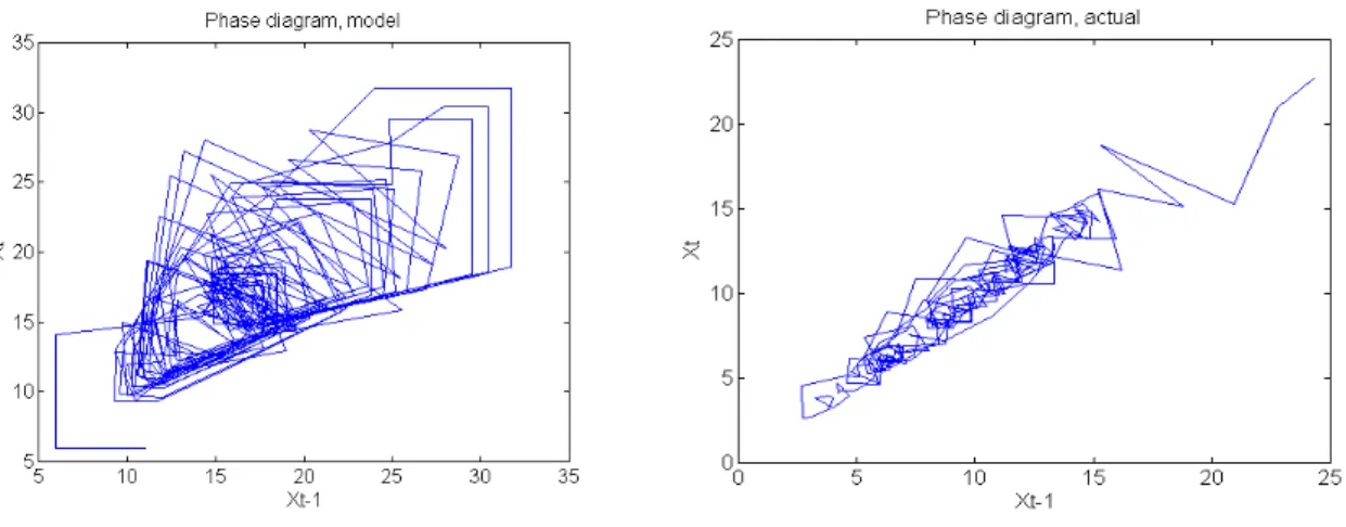
3°) The “model” series is significantly more volatile and “more periodic” than the actual one, as it is clear from the comparison of the autocorrelation functions (figure 2), and of the “phase diagram” (that is, xt as a function of xt-1) .
*******************Figure 2 Autocorrelation function for actual and simulated series ********************at about this place
******************Figure 3 : Phase diagrams of actual and simulated white sugar ******************price series at about this place
Policy lessons
Because it is made of 23 "regional" submodels, with, in each region, a representation of the behavior of a variety of agents, the model under examination provides also information on "who gains" and "who looses" from liberalization. The results presented here are illustrative. They are briefly exposed to show unexpected results that may arise from trade liberalization,
18The statistic given columns 3 and 4 is the ratio "BDS/standard deviation of the BDS under null hypothesis of
once innovative features, as exposed above, are introduced in a model of the sugar commodity chain 19/.
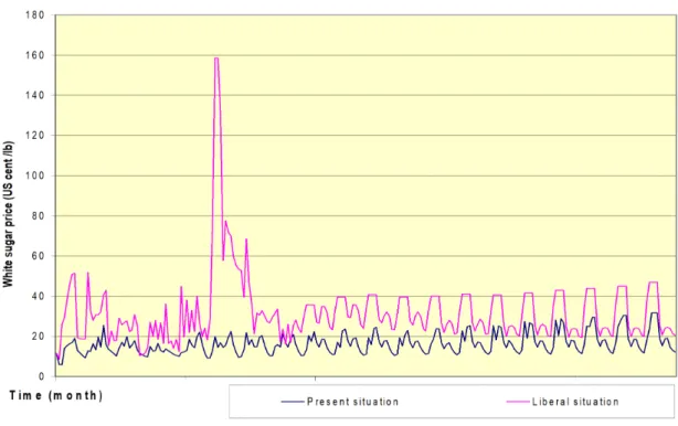
******************* Figure 4 : Comparison between “with” and “without” liberalisation about here
As shown by figure 4, price increases much after liberalization, and is becoming more volatile. Not surprisingly, governments loose, because imports taxes are suppressed. Farmers loose too (figure 5), except in a few third world countries (but their gains are extremely small by comparison with the losses of EC farmers), because, despite the mean price increase, the necessity of being cautious in presence of more volatile price leads to a reduction of production. Finally, most consumers loose also, (figure 6) because the reduction of production causes consumers prices to rise, even in some countries where high domestic prices were previously linked to protectionist policies.
******************Figure 5 - Effects of liberalization on farmers incomes, by country ************************about this place
*****************Figure 6 : Effects of liberalization on consumers, by country ************************about this place
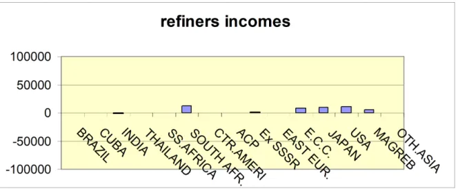
Are there any winners ? Some traders really can benefit from the liberalization, but not all of them (For instance, Brazilian traders suffer heavy losses20). The only indisputable
beneficiaries from liberalization are the refiners (figure 11), because the increased uncertainty increases the wedge between raw and white sugar, thus allowing them to get substantial profits 21/.
****************Figure 7 : Effects of liberalization on refiners, by country. ************************about this place
In any case, the overall result is rather negative, and the main reason for that is simply that, in the “liberal” situation, all agents being cautious, the increased volatility induces everybody to be prudent, and to produce only those quantity they are fairly sure to be able to sell. As a consequence, production is restricted (by comparison with the “present policy situation”), and almost everybody is worse off. This is a typical “prisoner’s dilemma”
19/ Throughout the rest of this paper, the consumer and producer surpluses are made use of as a proxy for a “true” social utility function. Of course, the authors are aware of the limitations of this indicator, which is “optimal” only under the heroic assumption that the income distribution is optimal, and that changes in prices do not change real incomes. Yet, despite its limitation, it is very commonly used, especially when making recommendation to policy makers. Hence our decision not to take another, more justified indicator.
20Without a large number of simulations, it is not possible to say whether this result is due to the specific
parameters or initial point chosen here, or if it is a permanent feature of the model.
21/ This is a natural consequence of the “ratchet effect” tied with refining capacity limitation. The point is noticed by WILLIAMS and ISHAM(1999).
situation, where self interest leads to collective catastrophe, just the contrary of the Adam Smith argument for “laisser faire” .
Conclusion
We have been able to set up a model of the world sugar commodity chain. It is firmly anchored into elementary economic theory. Yet, contrary to most “classical” models of the same kind, it assumes all agents risk averse, and expectations not always fulfilled, thus opening way to deviation from the otherwise automatically granted conclusion that “liberalization is good”. In effect, the main results are that:
1°) Price volatility may be much larger in a “ free trade ” than in a regulated environment.
2°) This implies a smaller average production, a higher average price, a smaller consumer surplus, and probably a smaller global welfare in most occasions.
3°) Such situations occurs as a consequence not of meteorological or other random events, but of endogenous fluctuations, built up from demand rigidity and traders imperfect knowledge. The remedy to such detrimental fluctuations cannot be found by the market itself. Suitable arrangements, combining as much liberty and as few bureaucracy as possible while correcting market inefficiencies must be sought for in such circumstances. It means obviously that the liberalization of the sugar market, if it were decided, should be conducted with much caution and prudence. Of course, this does not mean that the present situation is as fully satisfactory as it should.
One must be prudent in deriving practical conclusion from a notoriously imperfect model (but notice that most “ general equilibrium model ” did not even pass the rough test this one has been submitted to). The preceding conclusions should therefore be taken as a set of interesting hypothesis rather than policy recommendations. Yet, they should be taken seriously, and subject to additional investigations, if not for any other reasons, because of the precautionary principle.
More generally, if the tentative results just presented can be more strongly validated, contrary to a pervasive creed, the agricultural price regulation policies which were initiated by President Roosevelt in the aftermath of the great depression were not, or not only, the outcome of rent seeking agricultural lobbyists action 22/, but rather an efficient mean of
protecting consumers –especially, poor consumers.
Such findings call for further researches. By comparison with other crops, the originality of sugar lies in fact that production is regulated mainly thought quotas or “PEG”
(cf. HARVEY, 1989, among many other), which are costly to consumers, but not to
governments. The budgetary cost of sugar policies is therefore small, and the control of supply efficient. Yet, since it creates rents, and does not equate marginal cost to price, such
system is not justifiable from a static equilibrium point of view. For that reason, the idea of making use of similar schemes for other commodities, after having been contemplated in the 80’s, have been abandoned, and has disappeared from the landscape of agricultural policy discussions. What is shown by the present modeling experiment is that, in a dynamic setting, on the contrary, such a system makes much sense.
Actually, a PEG system can be interpreted as a sort of future market, with the State
promising to buy a certain (limited) quantity of commodity, at harvest time, at a prespecified price. The quantity thus bought by the State is then sold back to consumer, either at purchase price (in which case the consumer bear the cost of intervention) or at market price (in which case, the cost is taken by the taxpayer). If the commodity had been sold on a classical futures market, the cost would had been born exclusively by the consumer 23/. Apart for that faculty
of having the taxpayer bearing some of the cost instead of the consumer, the essence of both systems is the same. Especially, it may the argued that the allocative consequences are similar : the producer knows the selling price at plantation time, thus being comfortable in making a sound, riskless economic calculus. The distributional consequences, however, are not the same : because the State is risk neutral, it can provide this comfort at a much cheaper price than normal future markets, where risk buyers expect a reward from their contribution to risk reduction.
In the present state of thinking of the agricultural economist profession as a whole, this conclusion is so disturbing that it certainly deserve publication, in order to be discussed.
23/ Of course, in that case, the speculator, the one who sell the contract, loose from time to time. But unless he is
crazy, which contradicts the usual assumption of rationality, he cannot loose all the time. In the long run, he must have a profit. Otherwise, he would not speculate…
References
_____
ALLIGOOD, K., T.D. SAUER and J.A. YORKE (1977) : Chaos : an introduction to dynamical systems. Springer, New York.
BALE, M. and E. LUTZ (1979) : The effect of Trade intervention on international price
instability, AJAE 61 :
BAIROCH, P. (1992) : Le Tiers Monde dans l'impasse, Folio actuel, Gallimard, Paris.
BAIROCH, P. (1999) : Mythes et paradoxes de l’histoire économique, La Découverte, Paris.
BOURGES, B. (1998) : L’organisation commune du marché du sucre dans l’Union
Européenne, et les échanges mondiaux. Comptes rendus de l’Académie d’Agriculture de France, 84 (8) : 31-64.
BOUSSARD, J.M. (1996) : When risk generates chaos. Journal of Economic Behavior and Organization29 : 433-446.
BOUSSARD, J.M., and M.G. PIKETTY (2000) : Un modèle de l’industrie mondiale du sucre. Rapport de recherche, INRA-CIRAD, Paris (forthcoming).
BURTON, M. (1993) : Some illustration of chaos in commodity models. Journal of Agricultural Economics, 44 (1) 38-50.
CHAVAS, J.P. and M.T. HOLT (1993) : Market instability and non linear dynamic. American Journal of Agricultural Economics75 : 113-120.
COSTANZO, Sophie Di (2001) : Le rôle du stockage dans la dynamique des prix des matières premières. Thèse, Université de Paris I.
DEATON, A et G. LAROQUE (1992) : On the behaviour of commodity prices, Review of Economic Studies59 : 1-23.
DEHN, Jan (2001) : The effects on growth of commodity price uncertainty and shocks. Mimeo, University of Oxford.
FULPONI, L. (1994) : La variabilité des prix internationaux de base : les marchés sont-ils
efficaces ?Economie Rurale(219) : 16-23.
FULPONI, L. (1993) : Commodity price variability. Its nature and cause. OCDE, Paris.
GARDNER, B.L. (1992) : Changing economic perspectives in farm problem. Journal of Economic Literature 30 : 62-101.
GALIANI, F. (1770) : Dialogue sur le commerce des bleds. Réédition, Fayard, Paris 1984.
GRANGER, C.W.J (1966) : The typical spectral shape of an economic variable Econometrica
34 (1) :151-161.
HARVEY, D.R. (1989) : The GATT and Agriculture ; the production Entitlement Guarantee (PEG) option. Discussion paper 1/89, Department of Agricultural Economics and Food Marking, Newcastle upon type.
HAFI, A., P. CONNELL, and R. STURGISS (1993) : Market potential for refined sugar exports
from Australia. ABARE research reportsN°93-17, Canberra.
HOMMES, C., J. SONNEMANS, and H. VAN DE VELDEN (1998) : Expectation formation in a
cobweb economy : some one person experiment. Paper presented at the third workshop on economics with heterogenous interacting agents, Ancona, May.
JUST, R.E. and D. ZILBERMAN (1986) : Does the law of supply hold under uncertainty ? The Economic Journal, 96 : 514-524.
LEUTHOLD, R.M. and A. WEI (1998) : Long Agricultural Futures Prices : ARCH, Long Memory or Chaos processes ? ...Mimeo. OFOR papersN°98-3, May 1998.
LUCKE ,Bernt (1992) Price stabilization on world agricultural markets. An application to the
world market for sugar Springer Verlag, Berlin.
MALINVAUD, E. (1995) : Sur l’hypothèse de rationalité en théorie macro-économique Revue économique(46) : 523-536.
NERLOVE, M, D.M. GRETHER and J.L. CARVALHO (1995): Analysis of Economic Time Series: A Synthesis. Academic press, San Diego.
NEWBERY, D.M.G. and J. STIGLITZ (1981) : The theory of agricultural price stabilization. Clarendon Press, Oxford.
OLSON, M. (1965) : The logics of collective action public goods and the theory of groups. Cambridge, Mass., Harvard University Press.
PRATT, J.W. (1964) : Risk aversion in the large and in the small. Econometrica32 (1-2) : 122-136.
SHEALES T., GORDON S., HAFI A., TOYNE C (1999).. Sugar : Intervention policies affecting market expansion. ABARE Research Report N° 99.14., Canberra, 1999.
SCHUMPETER, J. (1954) : History of Economic Analysis Georges Allen and Unwin, London.
VOITURIEZ, T. (2000) : L’huile de palme et son marché : La modélisation de la volatilité. Thèse, Université de Paris I.
WILLIAMS, C.W., and B.A. ISHAM (1999): Processing Industry Capacity and the Welfare
Figure 1 : Comparison of actual and simulated white sugar world price over 240 months. ($ / tons)
Figure 2
Figure 5 - Effects of liberalization on farmers incomes, by country
Annex : Sugar model equations and parameters
I - Market module
[ Equations in this module are solved simultaneously each month (denoted by the subscript t) for bold capital variable. Some equations are generated for some values of the subscripts only: h(e,t) represents the set of region having harvest at time t ]
I.1/ Market equilibrium:
(I.1.1 : Supply equates demand): QQe + Qejt + Lejt = QFet + Cejt + ce.
Qejt: Quantity produced month t in region e, for sugar type j (j=”raw”, or “white”), in excess of quotas ; Cejt :
Quantity consumed, QFet demand from refinery (zero for white) ; Lejt: Net sales (may be negative) from stock;
QQe : Quota level for region e. ce : “forced” consumption(e.g. Brazil demand for alcohol);.
[Implicitely determines world sugar prices Pwt and Prt. ]
I.2/ Final consumption [e J(‘white’)]
(I.2.1: Consumers’model ): Ln ( [Cejt –ce]/ Net ) = e + eLn ( + Pejt[1+xe]) + eLn Iejt
Cejt (>ce): Quantity consumed ; Pejt equilibrium price in region e for time t; Iejt : Consumer income at time t
(=Ie0[1+iGe]t/12, with iGe: exogenous rate of growth); e e, , e : Country specific parameters. Net =Ne0( 1+ ge)t
population time t, ge :population rate of growth, country specific parameter; ce: “forced” consumption (e.g.
Brazil demand for alcohol); xe: region parameter, retail tax on sugar; e shift parameter (avoids P=0.0).
[ A standart constant elasticity demand function, with price and quantity constrained not to be nil ]
(I.2.2: Domestic consumer price definition) : Pejt = Max (P ejt , PQew) , j= “white”
Pejt equilibrium price in region e for time t; PQew: White sugar price under quota (exogenous).
[ As a rule, whenever quotas exist, domestic consumer price is linked with farm gate price under quota]
I.3/ Farmers
(I.3.1 : Production depends upon area) : QQe + Qejt = aj R2et DJet NFet
Qejt: Quantity produced in region e, for sugar type j (j=”raw”, or “white”), in excess of quotas; Ret Average
collection radius, region e, time t DJet : Sugar farming density, region e, time t NFet: : Number of processing plants
in region e, time t. aj : technical coefficient: Quantity of sugar in one ton of beet or cane; QQe : Quota level for
region e.
(I.3.2 : Farmers equilibrium) : aJeDJet= E( PJet) – AjeV(PJet)D2Jet
aJe : Farmer’s marginal cost (country parameter); DJet : Sugar farming density, region e, time t ; E( PJet) :
expected farm gate price for quantity in excess of quota (as promised by the processing plant); : Farmer risk
aversion coefficient (country parameter) ; V(PJet): Expected variance of farm gate price
[This equation is the farmer’s first order condition for Markowitz utility function maximisation with respect to
DJet, given R]
I.4 - Sugar processing plants [Defined for e,t h(e,t)]
(I.4.1: definition of processing margin): E( PJet) = TetE(P j)
[This equation relates the expected farm gate price with the expected equilibrium price. Notice Tet is a decision variable for processing plants]
(I.4.2: Expected sugar processing plants profit definition ):
E( BPet) = (Qjet E(P j) + QQePQje) (1 - Tet / aj ) – cje(Qjet + QQe) - cKe(Qjet + QQe) 3
E( BPet) : Expected processing unit profit (decision variable); Qjet:Processed quantity (decision variable) ;
E(Pej) : Expected world price for sugar j, year (j= “raw” or “white”) ; : Technical coefficient : cost of
processing one ton of “farm gate sugar”; CKe :Technical coefficient: cost of collecting one ton of “farm gate
sugar”, in t/km of average collection area ;Tet : Share of equilibrium price processing factories promise to pay
to farmers aj : technical coefficient: quantity of sugar in one ton of beet or cane; QQe: Quota level for region e; PQje: Guaranteed farm gate price under quota.
[ Notice the term in Q3, a consequence of the collection cost; ]
(I.4.3 : Variance of processors profit definition): V(BPet)= (1 – Tet / aj )2 Qjet2V(Pj)
V(BPet) : Expected variance of processing unit profit ; Tet : Share of equilibrium price processing factories
promise to pay to farmers; aj : technical coefficient: Quantity of sugar in one ton of beet or cane; QjetProcessed
quantity (decision variable); V(Pj) : expected price variance of processed product j
(I.4.4 : Utility of processing units): Uejt = E(BPet) - AFeV(Bet)
Uejt : Markowitz utility function of processing units; V(Bet) : Expected variance of processing unit profit ;
E(BPet): Expected processing unit profit (decision variable) ; AFe Risk aversion coefficient of processing units
[Deriving Uejt with respect to Qjet,, Tet, and Ret (after substitution from 3.5 and 3.4) provides three equations
(not listed here) which close the production module. In addition ,there exists a maximum capacity for processing units. Equation I.4.5 expresses this constraint, which results in a dual value Pjet being associated with
capacity]
(I.4.5: Capacity constraint ; Pjet associated variable) : Qjet < HPjet
I.5/- Stockpiling
(I.5.1: Accounting identity): Lejt = Sejt -Sejt+1
Letj: Net sales from stock month t, region e; Sejt: stock level in region e, month t, commodity j (It must be
noticed that : - < Letj <Sejt).
(I.5.2: Expected profit definition): E(BSejt) = PejtLejt +E(Pejt+1 ) Sejt+1 – KSejSejt+1
E(BSejt) Expected profit from stock; E(Pejt+1): Expected price for year t+1; Sejt: Stock month t, region e, sugar type
j ; Letj: Net sales from stock month t, region e; Pejt: equilibrium price for sugar type j, region e, month t. KSej:
stocking cost, exogenous parameter.
(I.5.3 : Stockpiling utility definition) : USejt = E(BSejt) - ASejV(Pejt+1)[ E(Pejt+1)Sejt+1]2
USejt: Stock decision maker utility; V(Pejt+1): expected variance of price of processed commodity j ; Sejt: stock
level in region e, month t, commodity j; E(BSejt): Expected profit from stock. ASej: Stock decision maker risk
aversion (exogenous parameter).
[Deriving USejt with respect to Sejt+1 and Letj , other variables assumed constant, provides two first order equation
(not listed here) determining sales and stocks]
I.6 /– Refinery
E (BRet ): Expected profit from refinery; QFet : Quantity processed by refinery time t; E(Pwt): Expected world
price for white sugar next month; Prt: equilibrium world price for raw sugar month t. aR : exogenous parameter,
rate of conversion of raw into white sugar; cRe: exogenous parameter, marginal cost of refinery in region e.
(I.6.2 : Variance of refinery profit definition ): V(BRet) =V(Pwt)QFet2
V(BRet) : Variance of refinery profit ; V(Pwt expected variance of white sugar equilibrium price; QFet : Quantity
processed by refinery time t;
(I.6.3 : Refiner utility function) : URet = E (BRet ) - AFe V(BRet)
URet : Refinery utility ; ARe: Refinery risk aversion coefficient ; E (BRet ): Expected profit from refinery. V(BRet): variance of refinery profit .
(I.6.4 : Capacity constraint) : QFet < HFet (associated dual value : Fet)
QFet : Quantity processed by refinery time t; HFet: Refinery capacity in region e, time t.
[Self explanatoty; Again, (6.3) is derived with respect to QFet under constraint (6.4) to get the equation
governing refinery behaviour; HFet is exogenous in module I ]
(I.6.5 : Ex post computation of actual profit): BRet = QFet(Pwt - aRPrt – HFet cRe)
BRet : actual profit, after equilibrium, therefore different from E(BRet); QFet :Quantity processed by refinery time t
Pwt : equilibrium white sugar world price; aR : exogenous parameter, rate of conversion of raw into white
sugar;Prt: equilibrium price of raw sugar; CRe: fixed cost for refinery. HFet: Refinery capacity in region e, time t
II – Capacity building module
[ This module is solved each year after harvest ,only if t h (e,t) . It determines refinery and processing capacity from existing capacity and new investments, by maximizing UJ subject to II.1 – II. 6]
(II.1 :Liquidity constraint) : wetIFe + wIeAIet < e BRet
e : : Parameter, saving propensity ; wIet : Parameter, cost of alternative ( non sugar) investments; wFe:
Parameter, cost of a new sugar factory,year t; BRet: Sugar refining industry actual profit, as computed from
module I; Iset: new sugar investment , year t; AIet: investment of sugar industry in alternative (non sugar)
sectors, year t; BRet Actual monthly profit, after equilibrium (comes from module I)
[standard equation for investment]
(II.2 : Capacity definition) : HFet = HFet-1 (1- dPe) + IFet , e, t
HFet: existing capacity year t ; Iset : new sugar investment , year t ;dPe: rate of depreciation
(II.4 : Utility) : UJ = E(WJ ) – AFe V(WJ)
UJ : Utility of investment portfolio; WJ : random value of portfolio; E(): expectation; V(): variance; AFe : refiners’
risk aversion coefficient .
[ Objective of a plain Markowitz portofolio model ]
(II.5: Expected return from investment ) : E(WJe) = E( Fet ) HFet+ AIet
HFet: Refinery capacity in region e, time t (endogenous in module II).
E(Fet) : Expected dual value of refinery capacity constraint ; : Riskless rate of interest.
(II.6 : Variance of return from investment): V(WJ) = V(Fet) HFet2
[Obviously]
III- Expectation module
[A base expected price PBis exoneously fixed througout time; Each month, this basic price is corrected
according to the situation; Expected variances are derived from expectations]
(III – 1 : Stock deviation from normality, definition) : Ssetj= (Setj- SNejt)/SNejt
Ssetj : current stock situation indicator ; Sejt: stock level in region e, month t, commodity j; SNejt: ‘normal’ level of
stock for commodity j, region e, month t
(III – 2 : Definition of monthly normal stock) : SNejt = t SEe/12
[ A “normal” stock after harvest is exogenously defined for each country; It should be consumed before next year]
(III- 3 : Price deviation from normality, definition) : PDejt = (Pejt-PB)/PB
PDejt: Price deviation for commodity j, region e, month t ; PB : exogenous “normal” price. Pejt : equilibrium price
(III – 3 : Mean price expectation ) : E(Pejt) = PB + PDejt(1- Ssejt) if PDejt0
= PB + PDejt Ssejt if PDejt <0 (III – 4 : Expected price variance) : V(Pejt) = [Pejt-1 - E(Pejt)]2
(III.5 : Processing plant expected annual price, mean ): E(PJet) = PB
(III.6 :Expected variance of annual price) : V(PJet) = (PB - Pejt-12)2;
Pejt equilibrium price in region e for time t; : Expected variance ;
[Thus, processing plants are insensitive to current price, but reactive to current price volatility ; Copied from Boussard (1996)]
(III.7 : Expected profitability of increasing capacity): E( Fet ) = Fet-1
III.8 : Expected variance of increasing capacity profitability): V(Pet) = ((Pet-1 - Pet-2)2
Fjet: profitability of expanding processing capacity, measured by the dual value associated with maximisation
problem I.4.2 through I.4.5;
[Naïve expectations; similar equations are written to define E(Fjet) and V(Fjet), profitability of increasing
Nature of production cane cane cane cane cane cane beet cane cane cane cane cane beet beet beet beet beet beet beet aJe, variable processing cost($/t) 100 30 50 30 40 30 100 50 50 90 30 90 40 50 100 100 90 40 40
Ck, fixed processing cost 20 5 10 10 5 15 15 5 20 15 5 5 5 5 25 20 15 5 5 Ct Transportation cost, $/t/km 0,1 0,5 0,3 0,3 0,2 0,6 0,2 0,4 0,4 0,1 0,3 0,4 0,4 0,4 0,1 0,1 0,1 0,3 0,4 AFe Processing plant risk aversion 0,01 0,01 0,1 0,1 0,01 0,1 0,01 0,1 0,1 0,01 0,01 0,1 0,02 0,1 0,02 0,01 0,01 0 0,1
Cj, farm gate cost (1000$/T) 51,3 6,3 30 5,4 17,1 0,79 17 2 3,3 32,2 0,771 1,5 4,5 4,5 7,9 7,5 46,9 3,6 0,52 Sf, average sugar surface per farm (Ha) 16,1 10 320 0 0,4 0,1 0,21 0 0,1 14,1 0,1 0,7 6,6 0,5 1 0,03 2,83 0,4 2,2
, farmers risk aversion parameter (1/$) 0,001 0,01 0,05 0,05 0,001 0,01 0,05 0 0,01 0 0,05 0,01 0 0 0,001 0 0 0,1 0,1 be White sugar price demand elasticity 0,16 0,02 0,07 0,3 0,29 0,07 0,03 0,1 0,07 0,04 0,13 0,01 0,01 0,2 0,05 0,13 0,04 0,1 0,1
ae Demand function constant -14,7 -3,7 -7 -21 -8,94 -14,7 -3,14 -8 -7,2 -14,6 -6,26 -12,7 -50 -50 -3,07 -15 -15 -6,3 -12,7
ge White sugar income demand elasticity 1,18 0,23 0,55 2,34 0,64 1,48 0,09 0,6 0,55 1,18 0,4 1 5,79 5,8 0,001 1,13 1,18 0,4 1
ee Demand function shift (X100) 1,7 16 4 0 0,5 1 7,2 3,1 5,31 3,7 4,3 0 21,2 21 1,2 0,9 3,8 4,3 0,33
KSej White stock maintenance cost ($/T) 20 10 10 15 15 10 20 10 10 20 10 15 15 15 20 20 20 10 15
KSej Raw stock maintenance cost ($/T) 20 10 10 15 15 10 20 10 10 20 10 15 0 0 0 0 0 0 0
de : saving propensity 0,05 0,05 0,05 0,05 0,05 0,05 0,05 0,1 0,05 0,05 0,05 0,05 0,05 0,1 0,05 0,05 0,05 0,1 0,05
Ne0 :Population year zero (Millions) 19,2 165 12 1000 61 530 40 310 8,5 300 360 1600 270 140 370 126 300 360 1600
gIe: GNP/head growth rate (%) 1,7 1,1 0,1 3 5,7 0,1 0,2 1 4 1,5 2 7 0,9 1 1,8 2,8 1,5 0,1 7
gpe : Population growth rate (%) 0,9 1,1 0,3 1,3 0,8 2,3 0,6 1,4 1,4 0,8 2,1 0,7 0,5 0,5 0,2 0,6 0,8 2,1 0,7
Iej0 GNP / head, year 0 (000$) 21 5,5 3 1,2 6,3 1,1 3,1 6 5,7 21 5 2,7 4,6 4,6 20 21 21 5 2,7
ARe Refinery risk aversion (1/$) 0,001 0,03 0,01 0,01 0,01 0,01 0,001 0 0,01 0 0,001 0,01 0,02 0,1 0,001 0 0 0 0,001
ASie=: Stockpiler risk aversion (1/$) 0,001 0,03 0,01 0,01 0,01 0,01 0,001 0 0,01 0 0,001 0,01 0,02 0,1 0,001 0 0 0 0,001
wPe factory cost ($/T of month. Cap.) 1200 500 500 600 600 500 1000 500 500 1250 500 500 500 900 1250 1250 1250 500 500
cRe : Variable cost for refinery ($/T) 125 80 80 80 80 80 100 80 80 125 80 80 100 100 125 125 125 80 80
QQe Production quotas (million T) 40 40 0 0 0 0 40 40 50 40 0 0 0 0 50 0 45 0 0
PQwe White price under quota ($/T) 430 430 0 0 0 0 430 430 580 430 0 0 0 0 700 0 500 0 0
PQie Farm price under quota ($/T) 40 40 0 0 0 0 40 40 50 40 0 0 0 0 50 0 45 0 0
WFe : Refinery cost ($/T of month cap.) 1200 500 500 600 600 500 1000 500 500 1250 500 500 500 900 1250 1250 1250 500 500
Parameters Level of quota (million T) White sugar price under quota ($/T) Farm gate price under quota ($ / T) x: retail tax on sugar (%) c: “forced” consumption (e.g. Brazil demand for alcohol) (Million T) Australia 0,005 430 40 0 0,02 Brazil 0,07 430 40 0 3,3 Cuba 0 0 0 0 0 India 0 0 0 0 0 Thailand 0 0 0 0 0 Africa, tropical 0 0 0 0 0 Africa, south 0,002 430 40 0 0,005 America, central 0,005 430 40 0 0,13 ACP countries 0,13 580 50 0 0,22 USA, cane 0,27 430 40 1 0 Maghreb, cane 0 0 0 0 0 Asia, cane 0 0 0 0 0 ex SSSR 0 0 0 0,45 0 Eastern Europa 0 0 0 0,45 0 Europe (EC) 0,145 700 50 1,8 3,625 Japan 0 0 0 2 0,2 USA, beet 0,11 500 45 0,7 0,9 Maghreb, beet 0 0 0 0 0 Asia, beet 0 0 0 0 0