Accuracy of predictive ability measures for survival models

(1)

HAL Id: hal-01552992

https://hal.sorbonne-universite.fr/hal-01552992

Submitted on 3 Jul 2017

HAL is a multi-disciplinary open access archive for the deposit and dissemination of sci-entific research documents, whether they are pub-lished or not. The documents may come from teaching and research institutions in France or abroad, or from public or private research centers.

L’archive ouverte pluridisciplinaire HAL, est destinée au dépôt et à la diffusion de documents scientifiques de niveau recherche, publiés ou non, émanant des établissements d’enseignement et de recherche français ou étrangers, des laboratoires publics ou privés.

Accuracy of predictive ability measures for survival

models

Philippe Flandre, Reena Deutsch, John O’Quigley

To cite this version:

Philippe Flandre, Reena Deutsch, John O’Quigley. Accuracy of predictive ability measures for survival models. Statistics in Medicine, Wiley-Blackwell, 2017, �10.1002/sim.7342�. �hal-01552992�

(2)

Research Article

Received 16 June 2016, Accepted 27 April 2017

(wileyonlinelibrary.com) DOI: 10.1002/sim.7342

Accuracy of predictive ability measures

for survival models

Philippe Flandre,

a*†

Reena Deutsch

b

and John O’Quigley

c

One aspect of an analysis of survival data based on the proportional hazards model that has been receiving increasing attention is that of the predictive ability or explained variation of the model. A number of contending measures have been suggested, including one measure,R2₍_{𝛽), which has been proposed given its several desirable}

properties, including its capacity to accommodate time-dependent covariates, a major feature of the model and one that gives rise to great generality. A thorough study of the properties of available measures, including the aforementioned measure, has been carried out recently. In that work, the authors used bootstrap techniques, particularly complex in the setting of censored data, in order to obtain estimates of precision. The motivation of this work is to provide analytical expressions of precision, in particular confidence interval estimates forR2₍_{𝛽). We}

use Taylor series approximations with and without local linearizing transforms. We also consider a very simple expression based on the Fisher’s transformation. This latter approach has two great advantages. It is very easy and quick to calculate, and secondly, it can be obtained for any of the methods given in the recent review. A large simulation study is carried out to investigate the properties of the different methods. Finally, three well-known datasets in breast cancer, lymphoma and lung cancer research are given as illustrations. Copyright © 2017 John Wiley & Sons, Ltd.

Keywords: predictive ability; prognostic factors; proportional hazards model; residuals; survival analysis

1. Introduction

Whereas the use of the Cox regression model in the analysis of censored survival data has become routine, the corresponding use of R2_{-type measures of explained variation is still not that common. Unlike the}

case of the linear model where there is essentially only a single contender, for survival models, there is more than one possibility. In an extensive review, Choodari-Oskooei et al [1, 2] examine the properties of a number of possible measures of R2 for survival data. Our purpose here is to add a piece to that development; this piece being the provision of a variance estimate for all of the measures discussed by [1]. One of our suggestions is rough and ready in that it is very easily calculated – coming under the heading of those techniques deemed desirable by student, techniques that ‘can be calculated on the back of a railway ticket while waiting for the train’ – but, as the simulations show, it may be too rough when the purpose is to obtain a reasonably accurate test. Nonetheless, agreement with the bootstrap calculations of [1] is generally good, and our suggestion is that it be used to obtain a rough interval estimate of the values compatible with an estimated R2_{. The general motivation for this variance estimate comes from the}

known approximately pivotal property of the Fisher’s transformation. Apart from this pivotal property, there is no other obvious reason why this coefficient should work so well, unless we take a linear model as a first approximation to the nonlinear Cox model, and it is a somewhat surprising result.

Aside from the Fisher transformation, we investigate analytical approximations for the variance of the

R2_{coefficients for survival data based on the proposals of [3]. There are two possible approaches here; the}

first makes use of the monotonicity relationship between the conditional expectation of an explained vari-ation measure and the regression coefficient,𝛽, and the second appeals to large sample approximations.

a_{Sorbonne Universités, UPMC Univ Paris 06, INSERM, Institut Pierre Louis d’épidémiologie et de Santé Publique (IPLESP}

UMR-S 1136), F75013 Paris, France

b_{Department of Psychiatry, University of California at San Diego, La Jolla, CA 92093, U.S.A.} c_{Laboratoire de Statistique Théorique et Appliquée, UPMC, Paris, France}

*Correspondence to: Philippe Flandre, Sorbonne Universités, UPMC Univ Paris 06, INSERM, Institut Pierre Louis d’épidémiologie et de Santé Publique (IPLESP UMR-S 1136) F75013 Paris, France.

(3)

Different transformations, aimed at local linearization, are considered. Local linearization corresponds to taking the first two terms of a Taylor expansion of R2_{around the maximum likelihood estimate, R}2_{( ̂}_𝛽).

Because such an expansion is available to us for any monotonic transformation of R2_{, we investigate}

some specific cases because some may linearize more successfully (more rapidly with sample size) than others. It is interesting to note good agreement between the different approaches and, also, good agree-ment with the results of [1] based on their use of the bootstrap. Somewhat like R2 _{itself, the goal is to}

give more an impression of overall strength of effect rather than something on which we might wish to base accurate error controlled decision-making.

Values of R2_{close to zero may still correspond to effects of interest, but we know that from the}

stand-point of individual prediction, there is much more noise than signal. Conversely, larger values may be such that the endeavour of building prognostic models that can be used effectively in practice becomes a plausible one. Thus, it would be helpful to provide interval estimates of R2or to at least be able to provide a reasonable range within which we might feel the actual value of predictive effect can be found. Note that such an interpretation would be close in spirit to a Bayesian one, rather than a more classical con-fidence interval interpretation, but, again, the goal is not to be so refined. It is more to have some rough and ready tools of service to us in our quest to build useful predictive models.

In the following section, we recall the basic structure of the main measure of our focus in this paper. The approximations, based on Taylor series, rely upon this structure and can therefore be seen as being specific to this measure. The Fisher transform on the other hand is very general and would apply to any measure, although we only study its performance in relation to the measure given in this section. Section 3 has two parts: the first part is devoted to Taylor series approximations for R2_{, as defined in Section 2,}

and some simple monotonic transformations of R2_{. The second part of Section 3 provides motivation and}

a simple expression for the variance of an invertible function of R2_{. The expression depends only upon}

R2_{, for which we use a plug-in estimate and the number of observed failure times. Section 4 presents}

a simulation to investigate coverage properties and how they might be influence by the size of the true population equivalent of R2_{, the rate of censoring, the distribution of the covariates and the correlation}

of the covariates in some relatively simple cases. Some real examples are considered in Section 5, and some further points of discussion are raised in Section 6.

2. R

2

measures for proportional hazards models

Let T denote the failure time, C the censoring time and Z(t) is p × 1 vector of explanatory variables. Assume that T and C are independent conditional on Z(t). Suppose the data consist of n independent replicates of (X, Δ, Z(t)), where X = min(T, C), Δ = I(T ≤ C), where I(⋅) is the indicator function. Let

Y_i(t) denote whether the subject i is at risk (Y_i(t) = 1) or not (Y_i(t) = 0) at time t. We will also use the counting process notation: let N_i(t) = I{T_i≤ t, T_i≤ C_i} and ̄N(t) =∑n_i=1N_i(t). The proportional hazards model [4] specifies that the hazard function for the failure time T associated with Z(t) takes the form

𝜆(t; Z(t)) = 𝜆0(t) exp(𝛽′Z(t)), (2.1)

where𝜆₀(.) is an unspecified hazard function and 𝛽 is a p × 1 vector of unknown regression parameters. The usual estimate, ̂𝛽, of 𝛽 is found by solving U(𝛽) = 0, where U(𝛽) is the score statistic of derivatives of the logarithm partial likelihood U(𝛽) =∑n_i=1Δ_ir_i(𝛽) where r_i(𝛽) are the partial Schoenfeld’s residuals at each observed failure of the time T_i, r_i(𝛽) = Z_i(t) −E_𝛽[Z|t] with

E_𝛽[Z|t] = n ∑ j=1 Z_j(t)𝜋_j(𝛽, t) , 𝜋_j(𝛽, t) = Yj(t) exp{𝛽 ′_Z j(t)} ∑n l=1Yl(t) exp{𝛽′Zl(t)} , (2.2)

the quantity𝜋_j(𝛽, t) being interpretable as the conditional probability that at time t, it is precisely individ-ual i who is chosen to fail, given all the individindivid-uals at risk and given that one failure occurs [3, 5]. When

𝛽 = 0, 𝜋i(0, t) is simply the empirical distribution of the covariate given t, assigning equal weight to each

sample subject in the risk set. In other words, given t and given the subjects in the risk set at t, we have a sampling model defined on this set by which every individual has the same probability of being selected. Shoenfeld residuals of the proportional hazards model [6] measure the discrepancy between the observed value of the covariate Z_i(t), from the individual i who fails at time t, and its expected value under

(4)

P. FLANDRE, R. DEUTSCH AND J. O’QUIGLEY

the model and that a single selection is being made from those subjects at risk. In the multivariate model (2.1), the dependence of the survival time variable on the covariates is via the prognostic index [5, 7]

𝜂(t) = 𝛽′_Z(t)_.

Two individuals with different Z’s but the same𝜂 should have the same survival probability. Let us define the quantityI(b) for b = 0, 𝛽 by

I(b) = n ∑ i=1∫ ∞ 0 {𝜂_i(t) −𝛽′E_b(Z|t)}2dN_i(t). (2.3) The measure of predictive ability of a proportional hazards model was therefore defined by [5]

R2(𝛽) = 1 −I−1(0)I(𝛽), (2.4)

where in practice,𝛽 is replaced by ̂𝛽. R2_{( ̂}_{𝛽) is a sample-based quantity which, under the usual asymptotic}

framework [7], converges to a population counterpart denoted Ω2₍_{𝛽) (details are outlined in O’Quigley}

and Xu where the properties of the coefficient were investigated). The ratioI( ̂𝛽)∕I(0) will approach 1 when there is almost no predictive effect and decrease towards the value 0 with increasing effect. We can generalize Schoenfeld’s residuals in the multivariate settings where for each observed failure time T_i, residuals are defined by w_i(𝛽) = {𝜂_i(t) −𝛽′_E

b(Z|t)} Then, in the case of a single covariate in the model,

residuals are a function of the Schoenfeld residuals with w_i(𝛽) = 𝛽 r_i(𝛽) and the predictive index in (2.4) reduced to the measure introduced by [3]

R2( ̂𝛽) = 1 − ∑n i=1Δir2i( ̂𝛽) ∑n i=1Δir2i(0) , (2.5)

where Δ_i = I(T_i ≤ C_i). Therefore, predictability or explained variability, in the context of proportional hazards regression, refers to predictability or variability of the value of the covariate, conditional upon the failure time and subjects at risk at that time. This approach has the great advantage of allowing us to consider the potential inclusion of time-dependent variables, which is one of the model’s most attractive features. The use of time-dependent variables not only is a key property of the model but also corresponds to many applied problems in chronic illnesses such as cancer and HIV. Although, in the context of survival data, it does seem more natural to want predictability to refer to time, because of the features of the model, in particular the importance of the residuals based on the value of the covariate, our approach is intuitively logical and has desirable properties [3, 5]. The exponentially tilted distribution given by equation (2.2) puts increasing weight on the higher values as the coefficient𝛽 increases. When 𝛽 assumes increasingly large negative values, then the same occurs on the smaller values. For a single binary explanatory variable, as𝛽 increases without bound, then all of the weight is put on the covariate value one. If we have perfect discrimination and the ones are systematically selected until they are exhausted, then as𝛽 → ∞, R2₍_{𝛽) → 1. If the zeros are selected until they are exhausted then, again, as 𝛽 → ∞,}

R2(𝛽) → 1. For a covariate taking on several values, or continuous, then, if at each observed failure time, the value of the covariate of the individual i who fail at T_i is the smallest (greatest) value among the sample values in the risk set, then the prediction is once more perfect and R2₍_{𝛽) = 1. Given the covariate,}

R2₍_{𝛽) increases monotonically in |𝛽| so that increasing strength of effect translates and increasing values}

of R2₍_𝛽).

3. Confidence interval estimates of R

2

(

𝛽)

3.1. Approximations based on linearization

For convenience, we denote R2₍_{𝛽) by R}2_{. R}2_{is a function of random variables Z}

1(t), … , Zk(t), where k

is the number of failures. We use Taylor series methods by expanding R2 _{through a series expansion to}

the first order so that we can obtain an estimate of Var(R2). For R2 = f (𝛽′Z₁(t), … , 𝛽′Z_k(t)) and letting

w_i_𝛽 = w_i(𝛽), w_i0= w_i(0), and𝜂_i=𝜂_i(t), i = 1, … , k, Var(R2) ≈ k ∑ i=1 { 𝜕R2 𝜕𝜂i }2 Var(𝜂_i) = k ∑ i=1 { 𝜕R2 𝜕Zij ∕𝜕𝜂i 𝜕Zij }2 Var(𝜂_i), (3.6)

(5)

where j = 1, … , p, where p is the dimension of the parameter space. These calculations are straightfor-ward and, after gathering terms, we have that

Var(R2) = k ∑ i=1 ⎡ ⎢ ⎢ ⎢ ⎣ 2Δ_iw_i𝛽∑Δ_jw2 j0− 2Δiwi0 ∑ Δ_jw2 j𝛽 (∑ Δ_jw2 j0 )2 ⎤ ⎥ ⎥ ⎥ ⎦ 2 Var(𝜂_i) = _(∑ 4 Δ_jw2 j0 )4 k ∑ i=1 Δ2_i [ w_i𝛽∑Δ_jw2_j0− w_i0∑Δ_jw2_j𝛽 ]2 Var(𝜂_i), (3.7) where Var(𝜂_i) is approximated by ∑p_j=1𝛽_j2Var(Z_ij(t)) + 2∑_j_<𝓁𝛽_j𝛽_𝓁 Cov(Z_ij(t), Z_i_𝓁(t)), Var(Z_ij(t)) =

E_𝛽[Z2

j|t]−E

2

𝛽[Zj|t], j = 1, … , p and Cov(Zij(t), Zi𝓁(t)) =E𝛽[ZjZ𝓁|t]−E𝛽[Zj|t]E𝛽[Z𝓁|t], j < 𝓁. Furthermore

letting S = log(1 − R2_), Var S ≈ k ∑ i=1 { 𝜕 log(1 − R2₎ 𝜕𝜂i }2 Var(𝜂_i) = k ∑ i=1 { 𝜕 log(1 − R2₎ 𝜕Zij ∕𝜕𝜂i 𝜕Zij }2 Var(𝜂_i), where j = 1, … , p. Again, gathering terms, we have that

Var[log(1 − R2)] = k ∑ i=1 [ 2Δ_i ( w_i_𝛽 ∑ Δ_jw2 j𝛽 −∑wi0 Δ_jw2 j0 )]2 Var(𝜂_i) =_(∑ 4 Δ_jw2 j0 ∑ Δ_jw2 j𝛽 )2 k ∑ i=1 Δ2_i [ w_i𝛽∑Δ_jw2_j0− w_i0∑Δ_jw2_j𝛽 ]2 Var(𝜂_i), In the same way, letting S∗_{= log(R}2_{∕(1 − R}2_{)), and regrouping terms, the variance of S}∗_{is approximated}

as Var(S∗_{) ≈} k ∑ i=1 [ 2Δ_i ( (w_i0− w_i_𝛽) ∑ Δ_jw2 j0− ∑ Δ_jw2 j𝛽 −_∑wi𝛽 Δ_jw2 j𝛽 )]2 Var(𝜂_i) =_((∑ 4 Δ_jw2 j0− ∑ Δ_jw2 j𝛽 ) ∑ Δ_jw2 j𝛽 )2 × k ∑ i=1 Δ2_i [ (w_i0− w_i_𝛽)∑Δ_jw2_j𝛽− w_i_𝛽(∑Δ_jw2_j0−∑Δ_jw2_j𝛽 )]2 Var(𝜂_i).

We first obtain a 95% confidence interval [S_L, S_U] and [S∗_L, S∗_U] for S and S∗, respectively. Then, the endpoints of these intervals were inserted into the transformed confidence interval for R2_{, [1−e}SU, 1−eSL]

and [eS∗ L∕(1 + eS ∗ L), eS ∗ U∕(1 + eS ∗

U)], by virtue of the monotonicity of S and S∗, respectively, as a function

of R2_.

3.2. Fisher’s transformation

Suppose we were to make a bivariate Edgeworth approximation to the joint distribution of T and Z. Obviously, we would need to make many more assumptions, in particular some parametric joint model for T and Z, but in fact, we will only need suppose that such a distribution exists. We will not carry out the calculation of the terms needed in the Edgeworth expansion, but we will suppose that they could be obtained if we had the joint model. The purpose of this is purely motivational, and in practice, the approximation we use is particularly simple and does not need any further calculation [8].

We take ̂𝜃 = tanh−1 R = 1 2log (_{1 + R} 1 − R ) ,

(6)

and, in the population,𝜃 = tanh−1Ω. Following the development of [9], it is possible to develop R as an infinite polynomial series in ̂𝜃 − 𝜃. We find, for a = ̂𝜃 − 𝜃,

f (a) = _√ nE(Δ) − 2 2𝜋(nE(Δ) − 1) [ 1 +a𝜃 2 + ( 2 +𝜃 8(nE(Δ) − 1)+ 4 −𝜃2 8 a 2₊nE(Δ) − 1 12 a 4 ) + ( 4 −𝜃2 16(nE(Δ) − 1)+ 4 + 3𝜃2 48 a 2₊n − 1 24 a 4 ) a𝜃 + ( 4 + 12𝜃2+ 9𝜃4 128(nE(Δ) − 1)2 + 8 − 2𝜃2+ 3𝜃4 64(nE(Δ) − 1)a 2₊8 + 4𝜃2− 5𝜃4 128 a 4 +(nE(Δ) − 1)28 − 15𝜃 2 1440 a 6 )]

exp −(nE(Δ) − 1)a2∕2.

Furthermore, neglecting powers of n higher than the third, for the first two moments, and higher than the forth for the next two, we have

E(a) = Ω 2(nE(Δ) − 1) [ 1 + 5 + Ω 2 4(nE(Δ) − 1)+ 11 + 2Ω2_{+ 3Ω}4 8(nE(Δ) − 1)2 ] (3.8) Var (a) = 1 nE(Δ) − 1 [ 1 + 4 − Ω 2 2(nE(Δ) − 1)+ 22 − 6Ω2_{− 3Ω}4 6(nE(Δ) − 1)2 ] . (3.9)

Given this result, we can calculate the first four moments, leading to

Var (𝜃 − tanh−1Ω) = 1

nE(Δ) − 1 +

4 −𝜃2

2(nE(Δ) − 1)2, (3.10)

which, in turn, can be approximated by (nE(Δ) − 1)−1+ 2(nE(Δ) − 1)−2= 1∕(nE(Δ) − 3). In practice, we do not know the value of E(Δ). We can though, under an independent censoring assumption, replace it by ̂Δ, defined as the proportion of failures in the sample scaled to the interval (0,1). This is once more a working assumption. In total then, for this rough and ready approximation, there have been a string of working assumptions. It is not easy to theoretically gauge the impact of these approximations on the usefulness of the final result and, so, rather than do that we simply investigated the performance of this approximation via a range of simulations. Also, of course, we were able to compare the results of the rough and ready approximation to those obtained via Taylor series expansion and the level of agreement was very satisfactory. Once we have the above intervals, we transform them back to the original scale for

R2_.

Asymptotically, E(𝜃) = tanh−1𝜌 and, approximately, var(𝜃) = 1∕(k − 3), where k is the number of deaths. We first obtain, a 95% confidence interval [𝜃_L, 𝜃_U] and then a 95% confidence interval for r, with

r =

√

R2_{( ̂}𝛽), [(e2𝜃L− 1)∕e2𝜃L+ 1), (e2𝜃U− 1)∕e2𝜃U+ 1)]. These intervals will not be symmetric, but they

are guaranteed to lie within the interval (0,1).

4. Simulations

A simulation study was conducted to evaluate the performance of the confidence intervals obtained using both Taylor series and Fisher’s transformation. For each simulation, a sample size of n = 100 or n = 400 was generated from an exponential distribution with parameter𝜆 = exp(𝛽₀ +𝛽z). The covariate z was a binary covariate either normally distributed or uniformly distributed with in all cases E[z] = 0.5 and Var[z] = 0.25. For example, for a binary covariate, z = 0 with probability 0.5 and z = 1 with probability 0.5 was generated. We investigated absence of censoring, and presence of 25%, 50% and 75% of censoring. The 95% confidence intervals of R2_{( ̂}_{𝛽) were calculated using all the methods presented}

previously, and the true value Ω2₍_{𝛽) was estimated as described in [3]. Five thousand replications of such}

samples were generated, and the coverage probability of each 95% confidence interval was calculated. A further simulation considered the case of bivariate normal covariables. The means and variances were the same as for the case of a single variable, and the correlation parameter took the values: 0.0, 0.3, 0.6 and

(7)

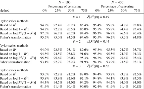
Table I.Simulation confidence intervals for R2_{with a binary covariate based on Taylor series methods}

and Fisher’s transformation.

N = 100 N = 400

Percentage of censoring Percentage of censoring

Method 0% 25% 50% 75% 0% 25% 50% 75%

𝛽 = 1 E[R2₍_{𝛽)] = 0.19}

Taylor series methods

Based on R2 _94.7% _93.7% _92.0% _86.5% _97.3% _95.9% _95.4% _93.3%

Based onlog[1 − R2_] _94.5% _93.8% _92.2% _87.5% _97.2% _95.8% _95.2% _93.5%

Based onlog[R2_{∕(1 − R}2_)] _97.8% _97.0% _96.4% _94.8% _97.5% _97.0% _96.7% _97.1%

Fisher’s transformation 95.8% 95.5% 94.9% 94.7% 96.9% 95.9% 95.3% 94.9%

𝛽 = 2 E[R2₍_{𝛽)] = 0.49}

Based on R2 _94.4% _93.6% _91.5% _88.1% _95.3% _94.8% _94.4% _92.8%

Based onlog[1 − R2_] _95.2% _94.7% _93.4% _91.1% _95.5% _95.1% _94.6% _93.5%

Based onlog[R2_{∕(1 − R}2_)] _95.8% _95.9% _95.6% _95.3% _95.6% _95.4% _95.3% _94.7%

𝛽 = 3 E[R2₍_{𝛽)] = 0.73}

Based on R2 _88.4% _87.8% _85.8% _83.6% _91.3% _90.3% _90.2% _88.3%

Based onlog[1 − R2_] _89.9% _90.3% _90.0% _92.6% _91.5% _90.7% _91.0% _90.8%

Based onlog[R2_{∕(1 − R}2_)] _90.5% _91.4% _91.0% _87.3% _91.7% _91.1% _91.7% _91.4%

Table II.Simulation confidence intervals for R2_{with a covariate normally distributed based on Taylor}

series methods and Fisher’s transformation.

N = 100 N = 400

Method 0% 25% 50% 75% 0% 25% 50% 75%

𝛽 = 1 E[R2₍_{𝛽)] = 0.19}

Based on R2 _94.2% _92.4% _90.2% _85.4% _95.4% _95.8% _94.7% _92.8%

Based onlog[1 − R2_] _94.2% _92.2% _90.5% _86.0% _95.5% _95.9% _94.4% _93.4%

Based onlog[R2_{∕(1 − R}2_)] _97.0% _96.7% _96.2% _94.4% _96.3% _96.9% _96.6% _96.4%

𝛽 = 2 E[R2₍_{𝛽)] = 0.44}

Based on R2 _94.0% _93.5% _93.1% _89.6% _95.8% _95.3% _94.7% _93.7%

Based onlog[1 − R2_] _94.8% _94.5% _93.8% _91.6% _95.8% _95.5% _94.9% _94.3%

Based onlog[R2_{∕(1 − R}2_)] _95.5% _95.6% _96.0% _95.3% _96.2% _95.7% _95.6% _95.4%

𝛽 = 3 E[R2₍_{𝛽)] = 0.62}

Based on R2 _93.0% _92.8% _91.2% _88.0% _94.4% _93.7% _93.2% _92.5%

Based onlog[1 − R2_] _93.8% _93.9% _92.6% _92.1% _94.8% _94.1% _93.9% _93.5%

Based onlog[R2_{∕(1 − R}2_)] _94.3% _94.5% _94.0% _94.2% _94.6% _94.2% _94.0% _94.0%

0.9. Sample sizes and censoring were as in the case of a single covariate. The impact of varying degrees of correlation is shown in the tables.

The results show that the confidence intervals based on Taylor series approximations for log[R2_{∕(1 −}

R2_{)] provide overall the most accurate coverage probabilities. This is true for all of the studied}

covari-ate distributions with a single variable (Tables I–III ). The results are satisfactory even for censoring as high as 75%. The simple Fisher’s transformation works well as a quick first approximation. Distribution of R2_{values for all simulations are provided in the Supporting Information. The limited study of}

corre-lation between the covariates is encouraging (Tables IV and V). The level of correcorre-lation appears to be well accounted for in the derived expressions. The Fisher transformation makes no use of the estimated

(8)

Table III.Simulation confidence intervals for R2 _{with a covariate uniformly distributed based on}

Taylor series methods and Fisher’s transformation.

N = 100 N = 400

Method 0% 25% 50% 75% 0% 25% 50% 75%

𝛽 = 1 E[R2₍_{𝛽)] = 0.19}

Based on R2 _92.0% _90.5% _90.3% _86.4% _94.9% _94.3% _93.7% _93.1%

Based onlog[1 − R2_] _92.0% _90.6% _90.3% _87.1% _94.7% _94.3% _93.7% _92.9%

Based onlog[R2_{∕(1 − R}2_)] _96.5% _96.7% _96.6% _95.1% _96.2% _95.6% _95.9% _97.1%

𝛽 = 2 E[R2₍_{𝛽)] = 0.45}

Based on R2 _93.6% _93.6% _92.3% _90.1% _95.2% _95.2% _95.2% _94.7%

Based onlog[1 − R2_] _93.8% _94.3% _92.7% _91.9% _95.3% _95.5% _95.3% _95.1%

Based onlog[R2_{∕(1 − R}2_)] _95.0% _95.5% _95.6% _96.1% _95.7% _95.8% _96.0% _96.1%

𝛽 = 3 E[R2₍_{𝛽)] = 0.64}

Based on R2 _92.6% _93.0% _91.2% _90.0% _94.2% _94.7% _95.0% _93.6%

Based onlog[1 − R2_] _93.6% _94.1% _92.8% _93.2% _94.4% _95.1% _95.2% _94.7%

Based onlog[R2_{∕(1 − R}2_)] _94.0% _94.9% _93.8% _95.1% _94.4% _95.2% _95.4% _95.1%

Table IV.Simulation confidence intervals for R2_{with two covariates normally distributed based on}

N = 100 𝜌 = 0 𝜌 = 0.3 𝜌 = 0.6 𝜌 = 0.9 Percentage of censoring Method 0% 50% 0% 50% 0% 50% 0% 50% 𝛽1=𝛽2= 0.5 E[R2₍_{𝛽)] = 0.13} E_[R2₍_{𝛽)] = 0.16} E_[R2₍_{𝛽)] = 0.18} E_[R2₍_{𝛽)] = 0.20}

Based on R2 _90.9% _89.5% _92.3% _90.1% _92.9% _90.4% _92.3% _91.4% Based onlog[1 − R2_] _90.7% _89.6% _92.1% _90.0% _92.7% _90.5% _92.3% _91.2% Based onlog[R2_{∕(1 − R}2_)] _96.2% _96.3% _96.8% _96.6% _96.7% _96.4% _96.6% _96.7% Fisher’s transformation 94.2% 95.5% 94.9% 95.3% 94.9% 95.1% 94.1% 95.0% 𝛽1=𝛽2= 1.0 E[R2₍_{𝛽)] = 0.32} E_[R2₍_{𝛽)] = 0.36} E_[R2₍_{𝛽)] = 0.41} E_[R2₍_{𝛽)] = 0.44}

Based on R2 _93.6% _92.9% _93.5% _93.1% _93.3% _92.1% _93.2% _91.5%

Based onlog[1 − R2_] _94.0% _94.2% _94.0% _94.1% _94.5% _93.3% _94.2% _93.1%

Based onlog[R2_{∕(1 − R}2_)] _95.0% _95.7% _95.0% _95.7% _94.9% _94.5% _94.5% _94.1%

correlations and, although it is less impressive than the Taylor series approximations, it still provides a good working guide for practical use. Here, these cases have been limited to bivariate normal, and it may be worth extending this study to deal with binary outcomes. It is less clear cut however how to carry out such studies because many different copula-type models could be suggested.

(9)

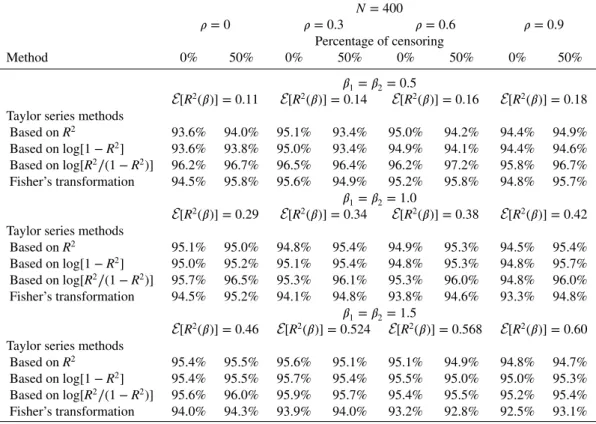
Table V.Simulation confidence intervals for R2 _{with two covariates normally distributed based on}

N = 400 𝜌 = 0 𝜌 = 0.3 𝜌 = 0.6 𝜌 = 0.9 Percentage of censoring Method 0% 50% 0% 50% 0% 50% 0% 50% 𝛽1=𝛽2= 0.5 E[R2₍_{𝛽)] = 0.11} E_[R2₍_{𝛽)] = 0.14} E_[R2₍_{𝛽)] = 0.16} E_[R2₍_{𝛽)] = 0.18}

Based on R2 _95.4% _95.5% _95.6% _95.1% _95.1% _94.9% _94.8% _94.7%

Based onlog[1 − R2_] _95.4% _95.5% _95.7% _95.4% _95.5% _95.0% _95.0% _95.3%

Based onlog[R2_{∕(1 − R}2_)] _95.6% _96.0% _95.9% _95.7% _95.4% _95.5% _95.2% _95.4%

5. Examples

Our first application is taken from [1] as we can easily calculate confidence intervals based on the Fisher’s transformation approach knowing the number of observed events and the measure estimate. Our results are in good agreement with those obtained using bootstrap method except for values larger than 0.9 (R2

PM,

R2_OF and R2_XO for the Leg ulcer study) where the Fisher’s transformation provided narrower confidence intervals and for values smaller than 0.25 where it provided larger confidence intervals (Table VI).

The Breast Cancer data involved 686 individuals with complete information of which 299 experienced the event of interest [10]. The final model suggested by [11] included age, tumour grade, number of positive lymph nodes, progesterone receptor and hormonal therapy [1]. Data were downloaded from http://www.homepages.ucl.ac.uk/ucakjpr/. The lymphoma data come from a study on diffuse large B cell lymphoma. The authors in [12] evaluated the extent to which the continuous Rosenwald gene score adds to the International Prognostic Index (IPI) in the prediction of survival in the 73 patients of the validation set for which the IPI values were available. Data were downloaded from http://llmpp.nih.gov/DLBCL/. For both studies, confidence intervals obtained using the Taylor approximations are in good agreement with those obtained via the Fisher’s transformation or those obtained by bootstrap methods (Table VII). Our last example is taken from [13] and is a set of 40 survival times for lung cancer patients, with seven covariates for each patient. The main purpose of the study was to compare the effects of two chemotherapy treatments in prolonging survival time, while assessing the effects of other factors such as age and months under treatment. Various analyses by [13] indicate that performance status is highly significant, and cell type is marginally significant; in particular, cell-type adeno is associated with an increased risk of failure. We then restrict attention to these two covariates having significant effects. Results are shown in Table VIII.

6. Discussion

Interest in predictive measures for survival models has grown in recent years. One reason for this comes from the need to quantify the impact on outcome of several, possibly a large number, of biomarkers or genetic information. The impact of markers can be subtle so that finding relevant effects leads us to careful

(10)

Table VI.Estimates of explained variation measures and 95% confidence intervals based on Fisher’s transfor-mation method and bootstraping.

Leg ulcer study Breast cancer study Lymphoma study

N events 97 299 48

N subjects 200 686 73

Measures Fisher Bootstrap Fisher Bootstrap Fisher Bootstrap

R2 PM 0.94 (0.91–0.96) (0.80–0.98) 0.27 (0.19–0.36) (0.21–0.35) 0.23 (0.05–0.45) (0.11–0.42) R2 OF 0.92 (0.88–0.95) (0.80–0.98) 0.37 (0.29–0.46) (0.30–0.46) 0.32 (0.11–0.54) (0.14–0.59) R2 XO 0.93 (0.90–0.95) (0.81–0.98) 0.38 (0.29–0.47) (0.30–0.48) 0.27 (0.08–0.49) (0.08–0.54) R2 D 0.52 (0.37–0.65) (0.44–0.65) 0.28 (0.20–0.37) (0.21–0.35) 0.23 (0.05–0.45) (0.11–0.40) R2 R 0.58 (0.44–0.70) (0.46–0.71) 0.29 (0.20–0.38) (0.23–0.38) 0.21 (0.04–0.43) (0.10–0.42)

Measures and bootstrap confidence intervals estimates obtained from [1]. The R2

OFof Choodari-Oskooei et al (2012a)

corresponds to our R2_{( ̂}_𝛽).

Table VII.Estimates of R2_{( ̂}_{𝛽) and 95% confidence intervals based}

on Taylor series methods and Fisher’s transformation method for breast cancer and lymphoma data.

Breast cancer study Lymphoma study

R2_{( ̂}_𝛽) _0.37 _0.32

Taylor series methods 95% CI of R2_{( ̂}_𝛽) _{95% CI of R}2_{( ̂}_𝛽)

Based on R2 _{(0.28–0.47)} _{(0.12–0.53)}

Based onlog[1 − R2_] _{(0.27–0.46)} _{(0.09–0.50)}

Based onlog[R2_{∕(1 − R}2_)] _{(0.29–0.47)} _{(0.16–0.55)}

Fisher’s transformation (0.28–0.46) (0.12–0.54)

Table VIII.Estimates of R2_{( ̂}_{𝛽) and 95% confidence intervals (CI) based on Taylor series}

methods and Fisher’s transformation method for lung cancer data.

Lung cancer study Variable ̂𝛽i R2( ̂𝛽1, ̂𝛽2) CI method 95% CI of R2( ̂𝛽1, ̂𝛽2)

Performance status −0.058 0.58 Based on R2 _{(0.35–0.81)}

Adeno 1.070 Based onlog(1 − R2₎ _{(0.27–0.76)}

Based onlog(R2_{∕(1 − R}2₎₎ _{(0.35–0.78)}

Fisher’s transformation (0.34–0.76)

consideration of both the fit and the predictive power of the models we use. Before dealing with the more subtle effects of biomarkers, it is important to correctly account for the prognostic role played by the more usual, often well-known, risk factors such as stage or grade of disease, age and other clinical factors that have been well studied. The effect of biomarkers can easily be masked or lost to uncertainty when we include the main clinical or demographic factors in any model, and so it is important to have some idea as to the precision of our predictive measures, given the main variables, before looking for more subtle effects. A very accurate assessment of this precision is not really necessary, but ballpark figures can indicate whether or not we have a good chance of picking up weaker effects. Goodness of fit plays a part here too. We have not considered that aspect in this work. Our results show quite good agreement with those obtained by Choodari-Oskooei [1]. An interval based on the Fisher transformation will be helpful in general situations. A simple application of the inverse hyperbolic tangent function, along with the added amount of predictive effect that we would like to be able to detect, leads to a direct assessment of the number of failures that we will need to observe. That can be of use in a sample size calculation or, otherwise, as an indicator of what we can reasonably hope to accomplish given the constraints of a particular study.

We find broad agreement with intervals obtained via bootstrap resampling. It might be argued that the effectiveness of the bootstrap obviates the need for more involved calculations. While there is something to be said for that viewpoint, we still think it is useful to have analytical expressions. The one based on the Fisher transform appears to perform remarkably well given its simplicity and it is simple enough to be

(11)

quickly evaluated by hand, or even mentally, in the context where computer-based resampling may not be readily available. Some reassurance can be obtained from the fact that there is broad agreement between all of the approaches. Nominal coverage of the confidence intervals cannot be described as highly accurate but is nonetheless good and exhibits only a very weak dependence, if any, on the strength of association itself, the degree of censoring and the amount of correlation between the variables, at least in the limited cases studied. Improvements are very likely possible but because our purpose is one of obtaining a rough ballpark guide rather than one of high accuracy, the extra investment in calculation may not be justified.

Acknowledgements

The authors would like to thank the editors and reviewers for a detailed review of an earlier version of this work. In particular, we would like to thank them for having identified an important error in the development.

References

1. Choodari-Oskooei B, Royston P, Parmar MKA. Simulation study of predictive ability measures in a survival model I: explained variation measures. Statistics in Medicine 2012; 31:2627–2643.

2. Choodari-Oskooei B, Royston P, Parmar MK. A simulation study of predictive ability measures in a survival model II: explained randomness and predictive accuracy. Statistics in Medicine 2012; 31:2644–2659.

3. O’Quigley J, Flandre P. The predictive capability of proportional hazards regression. Proceedings of the National Academy

of Sciences of the United States of America 1994; 91:2310–2314.

4. Cox DR. Regression models and life tables (with discussion). Journal of the Royal Statistical Society B 1972; 34:187–220. 5. O’Quigley J, Xu R. Explained variation in proportional hazards regression. In Handbook of Statistics in Clinical Oncology,

Crowley J (ed.) Marcel Dekker: New York, 2001; 397–409.

6. Schoenfeld DA. Partial residuals for the proportional hazards regression model. Biometrika 1982; 69:239–241.

7. Andersen P K, Gill R D. Cox’s regression model for counting processes: a large sample study. Annals of Statistics 1982;

10:1110–1120.

8. Deutsch R. Survival Prediction Following HIV Infection: Interval Censored Infection Times and Subsequent Cognitive

Impairment and Mortality. University of California: San Diego, 1996. 9714837.

9. Fisher R. On the ‘probable error’ of a coefficient of correlation deduced from a small sample. Metron 1921; 1:3–32. 10. Schumacher M, Bastert G, Boja H, Hübner K, Olschewski M, Sauerbrei W, Schmoor C, Beyerle C, Neumann RL,

Rauschecker HF. Randomized 2 × 2 trial evaluating hormonal treatment and the duration of chemotherapy in node-positive breast cancer patients. German Breast Cancer Study Group. Journal of Clinical Oncology 1994; 12:2086–2093. 11. Sauerbrei W, Royston P. Building multivariable prognostic and diagnostic models: transformation of the predictors by

using fractional polynomials. Journal of the Royal Statistical Society (Series A) 2002; 162:71–94.

12. Dunkler D, Michiels S, Schemper M. Gene expression profiling: does it add predictive accuracy to clinical characteristics in cancer prognosis? European Journal of Cancer 2007; 43:745–751.

13. Lawless JF. Statistical Models and Methods for Lifetime Data. Wiley: New York, 1982.

Accuracy of predictive ability measures for survival models

HAL Id: hal-01552992

https://hal.sorbonne-universite.fr/hal-01552992

Accuracy of predictive ability measures for survival

models

Philippe Flandre, Reena Deutsch, John O’Quigley

To cite this version:

Research Article

Accuracy of predictive ability measures

for survival models

Philippe Flandre,

Reena Deutsch

and John O’Quigley

1. Introduction

2. R

measures for proportional hazards models

3. Confidence interval estimates of R

(

𝛽)

4. Simulations

5. Examples

6. Discussion

Acknowledgements

References

Supporting information