Computation of upper and lower bounds in limit analysis using second-order cone programming and mesh adaptivity

(1)

Computation of Upper and Lower Bounds in Limit Analysis using Second-order Cone Programming and Mesh Adaptivity

by

H´ector Ciria Su´arez

Ingeniero de Caminos, Canales y Puertos (2002) Universidad Polit´ecnica de Catalu˜na, Barcelona, Spain

Ing´enieur des Ponts et Chauss´ees (2002) ´

Ecole Nationale des Ponts et Chauss´ees, Paris, France Submitted to the Department of Aeronautics and Astronautics

in partial fulfillment of the requirements for the degree of Master of Science in Aeronautics and Astronautics

at the

MASSACHUSETTS INSTITUTE OF TECHNOLOGY May 2004

c

Author . . . . Department of Aeronautics and Astronautics

May 14, 2004 Certified by. . . . Jaime Peraire Professor Thesis Supervisor Accepted by . . . . Edward M. Greitzer H.N. Slater Professor of Aeronautics and Astronautics Chair, Committee on Graduate Students

(2)

(3)

Computation of Upper and Lower Bounds in Limit Analysis using Second-order Cone Programming and Mesh Adaptivity

by

H´ector Ciria Su´arez

Submitted to the Department of Aeronautics and Astronautics on May 14, 2004, in partial fulfillment of the

requirements for the degree of

Master of Science in Aeronautics and Astronautics

Abstract

Limit analysis is relevant in many practical engineering areas such as the design of mechanical structures or the analysis of soil mechanics. Assuming a rigid, perfectly-plastic solid subject to a static load distribution, the problem of limit analysis consists of finding the minimum multiple of this load distribution that will cause the body to collapse. This collapse multi-plier results from solving an infinite dimensional saddle point problem, where the internal work rate is maximized over an admissible set of stresses -defined by a yield condition- and minimized over the linear space of kinematically admissible velocities for which the external work rate equals the unity. When strong duality is applied to this saddle point problem, the well-known convex (and equivalent) static and kinematic principles of limit analysis arise.

In this thesis, an efficient procedure to compute strict upper and lower bounds for the exact collapse multiplier is presented, with a formulation that explicitly considers the exact convex yield condition. The approach consists of two main steps. First, the continuous problem, under the form of the static principle, is discretized twice (one per bound) by means of different combinations of finite element spaces for the stresses and velocities. For each discretization, the interpolation spaces are chosen so that the attainment of an upper or a lower bound is guaranteed. The second step consists of solving the resulting discrete nonlinear optimization problems. Towards this end, they are reformulated into the canonical form of Second-order Cone Programs, which allows for the use of primal-dual interior point methods that optimally exploit the convexity and duality properties of the limit analysis model and guarantee global convergence to the optimal solutions.

To exploit the fact that collapse mechanisms are typically highly localized, a novel method for adaptive meshing is introduced based on local bound gap measures and not on heuristic estimates. The method decomposes the total bound gap as the sum of positive elemental contributions from each element in the mesh, and refines only those elements which are responsible for the majority of the numerical error. Finally, stand-alone computational cer-tificates that allow the bounds to be verified independently, without recourse to the original computer program, are also provided. This removes the uncertainty about the reliability of the results, which frequently undermines the utility of computational simulations.

The efficiency of the methodology proposed is illustrated with several applications in plane stress and plane strain, demonstrating that it can be used in complex, realistic prob-lems as a supplement to other models.

Thesis Supervisor: Jaime Peraire Title: Professor

(4)

Acknowledgments

This work would have never been possible without the support, dedication and help of many people towards who I feel deeply grateful.

First of all, I am indebted to my advisor, Prof. Jaime Peraire, for his successful guidance in my research, excellent academic and technical advise and for his outstanding intuitions and constant encouragement. But, above all this, I am grateful to him for his friendship and valuable personal advices that I will never forget. His permanent good mode and faith in my work made working with him always a pleasure.

Thanks also to Prof. Dimitris Bertsimas for his suggestions about Second-order Cone Programming and to Prof. Rob Freund for answering questions about convex optimization. Thanks to Prof. Antonio Huerta for offering me the possibility to continue my research in Barcelona during the summer period. Special thanks deserves Per-Olof Persson, whose deep knowledge about Matlab enabled my codes to run much faster than expected. I am also grateful to Nuria Pares for allowing me to use some of her subroutines. Ms. Jean Sofronas, whose dedication and efficiency made everything easier at MIT, is also thankfully acknowledged.

I cannot think about this work without remembering many of the ACDLers, the people from my lab. Thanks to David for his funny Québécois accent, his chess lectures and for sharing with me his passion about ice hockey. Thanks also to Matthieu and Todd for the squash games, and for his permanent availability to discuss about irrelevant issues. Ryan deserves also my recognition for his unconditional faith in the Red Sox. Each time they lost in Fenway Park, I could see in him the same frustration I experienced with the defeats of my loved FC Barcelona, my soccer team. Thanks also to Garrett, not only for being a computer wizard that solved all my problems whenever Linux did not collaborate, but also for calling me at 7am to go to the gym every other morning. Finally, thanks also to Ian, Jérôme, Thomas and the remaining French community.

Outside MIT, Paula, Laura and Mariu brought to my life an Argentinean flavor that transformed my weekends into holidays in Buenos Aires. They offered me a friendship that, I hope, will follow, and were the contact through which I met many other people from Harvard, Tufts, BU, etc. I wish all the best for them in the future.

My last words will be for my parents, Francisco and Lourdes, and my sister, Laura. I am more than grateful for their support and for encouraging me whenever I needed motivation. Although I was an ocean away, I always felt close to them.

The work reported in this thesis was made possible by the financial support of the Singapore-MIT Alliance.

(5)

List of Figures

1-1 Linear elastic and limit analysis solutions for a given example . . . 13

2-1 Rigid, perfectly-plastic behavior . . . 17

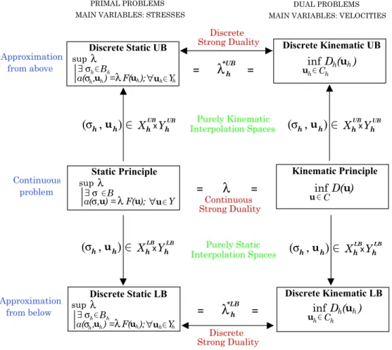
2-2 The use of purely static and purely kinematic finite element spaces to obtain lower and upper bounds for the collapse multiplier . . . 26

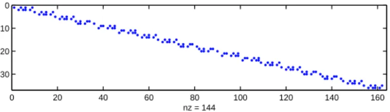
4-1 Illustration of the block structure and sparsity of matrix Aeq1 _{. . . .} ₄₁

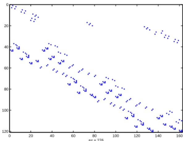
4-2 Trivial mesh and boundary conditions to illustrate the sparsity of the matrices involved in the bound problems. The mesh has 18 elements, 16 nodes, 3 Dirichlet edges ξD e , 9 Neumann edges ξeN and 21 interior edges ξe 0 e . . . 41

4-3 Illustration of the structure and sparsity of matrix Aeq2 _{. . . .} ₄₃

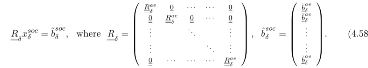
4-4 Illustration of the structure and sparsity of the global matrix for the lower bound problem . . . 45

4-5 Comparison of the size of the global lower bound matrix for problems (4.48) and (4.59) . . . 49

4-6 Illustration of the structure and sparsity of the matrix Aeq_{. . . .} ₅₄

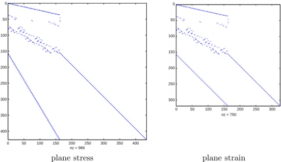
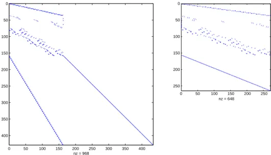
4-7 Illustration of the structure and sparsity of the global matrix for the upper bound problem in plane stress and plane strain. . . 57

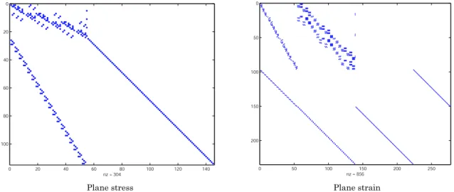
4-8 Notation for the elemental bound gap ∆e h . . . 63

5-1 Geometry and loads for the cantilever problem in plane stress . . . 68

5-2 Cantilever problem - Deformed geometry using uniform meshing . . . 69

5-3 Cantilever problem - Nodal velocities . . . 69

5-4 Cantilever problem - Convergence using uniform meshing . . . 69

5-5 Cantilever problem - Deformed geometry using adaptive meshing . . . 71

5-6 Cantilever problem - Elemental contribution to the bound gap ∆e h . . . 71

5-7 Cantilever problem - Adaptive meshing strategy: elements to be refined . . . 71

5-8 Cantilever problem - Bounds using adaptive meshing . . . 72

5-9 Cantilever problem - Comparison of adaptive versus uniform meshing . . . . 72

5-10 Cantilever problem - Elemental measure of deformation||εe h|| . . . 74

(8)

5-11 Cantilever problem - Alternative adaptive meshing strategy: elements to be

refined . . . 74

5-12 Cantilever problem - Bound gap rate of convergence for different adaptive meshing strategies . . . 74

5-13 Geometry and loads for the slotted block problem in plane stress . . . 75

5-14 Slotted block problem 1 - Deformed geometry using uniform meshing . . . 76

5-15 Slotted block problem 1 - Nodal velocities . . . 77

5-16 Slotted block problem 1 - Convergence using uniform meshing . . . 77

5-17 Slotted block problem 1 - Deformed geometry using adaptive meshing . . . . 78

5-18 Slotted block problem 1 - Adaptive meshing strategy: elements to be refined 79 5-19 Slotted block problem 1 - Bounds using adaptive meshing . . . 79

5-20 Slotted block problem 1 - Comparison of adaptive versus uniform meshing . . 79

5-21 Geometry and loads for the beam problem in plane strain . . . 80

5-22 Beam problem - Deformed geometry using uniform meshing . . . 81

5-23 Beam problem - Convergence using uniform meshing . . . 82

5-24 Beam problem - Deformed geometry using adaptive meshing . . . 83

5-25 Beam problem - Elemental contribution to the bound gap ∆e h . . . 83

5-26 Beam problem - Adaptive meshing strategy: elements to be refined . . . 83

5-27 Beam problem - Bounds using adaptive meshing . . . 84

5-28 Beam problem - Comparison of adaptive versus uniform meshing . . . 84

5-29 Geometry and loads for the slotted block problem in plane strain . . . 85

5-30 Slotted block problem 2 - Deformed geometry using uniform meshing . . . 87

5-31 Slotted block problem 2 - Upper and lower bounds using uniform meshing . . 87

5-32 Slotted block problem 2 - Rates of convergence using uniform meshing . . . . 89

5-33 Slotted block problem 2 - Deformed geometry using adaptive meshing . . . . 89

5-34 Slotted block problem 2 - Bounds using adaptive meshing . . . 90

(9)

List of Tables

5.1 Results for the cantilever problem in plane stress using uniform meshing . . . 68 5.2 Results for the cantilever problem in plane stress using adaptive meshing . . 70 5.3 Results for the cantilever problem in plane stress using an alternative,

deformation-based, adaptive meshing strategy . . . 75 5.4 Results for the slotted block problem in plane stress using uniform meshing . 76 5.5 Results for the slotted block problem in plane stress using adaptive meshing . 78 5.6 Results for the beam problem in plane strain using uniform meshing . . . 81 5.7 Results for the beam problem in plane strain using adaptive meshing . . . 82 5.8 Results for the slotted block problem in plane strain using uniform meshing . 88 5.9 Results for the slotted block problem in plane strain using adaptive meshing . 91 5.10 Computational cost of solving the lower and upper bound problems for the

finest uniform and adaptive meshes used in all previous examples . . . 93 6.1 Overview of different, recent approaches in limit analysis . . . 97

(10)

(11)

Chapter 1 Introduction

1.1 Motivation of Limit Analysis and Previous Work

The theory of limit analysis assumes a rigid, perfectly-plastic material to model the collapse of a solid that is subject to a static load distribution. Due to the rigid assumption on the ma-terial, small forces are neutralized by stresses without incurring in any elastic deformation. Therefore, these stresses are not governed by a constitutive equation and, consequently, they are not uniquely determined by the equilibrium equation. When the forces are sufficiently large, the stresses within the material, which are limited by a yield condition, cannot neu-tralize the forces without incurring in a permanent, plastic deformation. Then, the material is said to be flowing and will continue to flow permanently as long as the forces remain and the geometric changes are ignored. Thus, the deformation of the material is described in terms of velocities or flows, and not by displacements, as is usually the case in elastic models. Clearly, the model of limit analysis corresponds to a very simplified situation of a rigid-plastic material and static or slowly increasing loads. However, it makes it possible to analyze quantitatively the plastic collapse of a material. It is worth mentioning that the model only describes the fields of stresses and velocities in the exact moment when collapse first occurs. Therefore, it does not give information about what happens once the deformation modifies the initial geometry. In this sense, limit analysis gives a snapshot of the collapse moment.

Within this context, the problem of limit analysis is the following: consider a continuum subject to a fixed force distribution consisting of both volume and surfaces loads. Then, the objective is to obtain the minimum multiple of this force distribution that causes the collapse of the body, i.e., the multiple for which plastic flow first occurs. Usually, this multiple is named the collapse multiplier. At the same time, one may be interested in the fields of stresses and velocities that are present in the body at collapse. Likewise, it might be of interest to know the plastified region, i.e., the part of the body where the stresses are at the limit and plastic deformation is occurring.

(12)

linear elasticity, and goes beyond the scope of the latter. The model of linear elasticity is simple because it results in a linear elliptic boundary value problem, which behaves very well both from a mathematical and a numerical point of view. This permits to solve realistic problems in great detail. However, it is well known that even small forces might cause locally unbounded elastic stresses, which do not adjust to the physical reality. Therefore, some plastic analysis needs to be performed to obtain realistic predictions that can satisfy the more and more demanding engineering design requirements. This is the motivation underlying collapse analysis. Indeed, from the perspective of computational methods, the goal is to make limit analysis applicable to complex, realistic engineering problems as a supplement to the elastic treatment, which is nowadays a standard tool in engineering.

However, limit analysis is more complex. The continuous problem corresponds to an infinite dimensional saddle point problem of a bilinear form (internal work rate) in stresses and velocities. In particular, the bilinear form is maximized over a space of admissible stresses -defined by a yield condition- and minimized over the linear space of kinematically admissible velocities for which the external work rate is constant. The presence of the yield condition introduces nonlinearity in the problem, which represents an important difficulty and the major difference with the elastic model. The good news is that nice strong duality properties hold for this saddle point problem. In fact, when duality is applied to the problem, the well-known static and kinematic principles of limit analysis arise, as shown in [14] or [15]. These principles, upon which are based the classical lower and upper bound theorems of limit analysis (see [22]), are convex and only involve in their respective formulation either stresses (static principle) or velocities (kinematic principle).

In the numerical solution process for both the elastic and the limit analysis models, the first step is to discretize their corresponding continuous problems by the introduction of finite dimensional Sobolev spaces. However, in limit analysis, uniqueness and regularity do not hold, unlike in the theory of elliptic boundary value problems. From a numerical perspective, mixed finite elements are typically used and special care must be paid to the interpolation spaces employed for the stresses and the velocities. Moreover, whereas in linear elasticity the discrete problem results in a simple linear system of equations, in limit analysis (and because of the yield condition) one must solve a large nonlinear optimization problem, which represents the major difficulty and challenge in the solution process.

Solving this optimization problem is the second important step. Typically, the methods used are based on iterative processes that require the solution, in each iteration, of sparse linear systems of equations of larger complexity than those appearing in the linear elastic problems. Finally, the convergence results for the numerical solution are weaker than in the elastic case. However, and despite the difficulties mentioned, the recent advances in convex optimization enable limit analysis to be applied, nowadays, to realistic applications.

To close the comparison between linear elasticity and limit analysis, we find it illustrative to solve the same problem with each theory. Figure 1-1 shows, graphically, the problem

(13)

Limit Analysis Elasticity Theory

1

L = 1

Η = 0.5

Figure 1-1: Linear elastic and limit analysis solutions for a given example

considered and the elastic and plastic deformations obtained. Notice that, in limit analysis, the solution allows for discontinuous, infinite deformations, but the stresses must (in general) be bounded.

As previously pointed out, the nonlinearity introduced by the yield condition in the limit analysis formulation is an important source of difficulty when solving the resulting discrete optimization problem. Traditionally, the way to overcome this difficulty was to linearize the convex yield condition, thereby obtaining a polyhedral approximation to the yield surface. This formulation was firstly introduced in the early seventies in [26]. Then, the resulting problem reduces to a classical linear program (LP): see, for instance, [2, 13, 14], based on the Simplex method or, more recently, [4, 17] using Interior Point Methods (IPM). Although this approach has been used extensively in two dimensions, its application to three dimensions is highly hampered by the fact that the number of constraints generated in the linearization process increases dramatically, thereby increasing also the computational cost.

The first attempts to solve for the exact convex yield condition were addressed in [11] and [31]. However, only cases with bounded yield sets on very coarse meshes were considered1. Although some progress was made in [15] -using a nonlinear programming package to the static principle of limit analysis- and also in [10, 12] -developing methods to solve the convex yield condition-, all the computational results were limited to moderate size grids (no more than 1000 elements). Successful results on fine grids (more than 10000 elements) for exact quadratic, von Mises-type yield conditions were first possible in [7], by exploiting duality and extending the ideas of IPMs for LP to the minimization of sum of norms (MSN), which is a particular case of a Second-order Cone Program (SOCP) [25]. The main drawback of the approach was that, for unbounded yield sets, the incompressibility constraint on the flow required the use of very cumbersome finite element spaces. This was overcome in [16], using [5] to solve the nonlinear optimization problem. Thus, the method in [16] makes finally

1_{The unboundness of the yield condition, which appears in many important cases (for instance, in the von}

Mises plane strain or three-dimensional models), is an additional complication since it requires incompress-ibility in the flow field to be imposed.

(14)

possible to solve large problems, including the important cases of unbounded yield sets, for the exact convex yield condition (although restricted to von Mises-type yield criteria). In [18], automatic mesh refinement is introduced to improve the method in [16], and using [6] as the optimization solver. Despite improving the efficiency of [16], the strategy used for automatic mesh refinement does not rely on local error measures but in heuristic estimates. Consequently, its performance is far from optimal.

An important feature of the references mentioned above (except for the old approaches given in [2] and [11], that were based on the bound theorems) is that they only provide ap-proximations to the collapse multiplier, but do not yield strict bounds. Therefore, although the approximate values given by those methods might be accurate, the lack of certainty on the error incurred is a serious drawback. Uncertainty about the reliability of numerical simulations in engineering usually leads to computations that are much more expensive than strictly necessary, in an attempt to trust the results. The lack of guarantee creates doubts when discrepancies arise and, more importantly, prevent the numerical solutions to be certi-fied. For these reasons, the possibility of computing bounds of the limit loads, and not only estimates, has a very relevant added value in today’s engineering.

In [23, 24], upper and lower bounds of the collapse multiplier are computed for soil me-chanics problems using linear finite elements and a two-stage, quasi-Newton optimization algorithm. This algorithm is based on the nonlinear programming schemes developed in [37] to solve limit analysis problems arising from a mixed formulation. Although the method seems to be applicable to all convex yield surfaces, smoothness is required since first and second order derivatives of the yield function need to be computed. The efficiency of the method is mainly documented for a smooth approximation of the Mohr-Coulomb yield func-tion, on uniform meshes. The solution method is not unified, since upper and lower bounds are obtained by different versions of the quasi-Newton method, whose performance seems to rely on some heuristics. Moreover, duality is not exploited, thereby preventing the method from gaining additional efficiency and robustness.

A new recent approach to obtain lower bounds, without the need to linearize the yield criteria, is presented in [21]. It uses an IPM that exploits the convexity and duality properties of limit analysis. Moreover, the method is general in the sense that no particular finite element discretization or yield criterion is required. However, only a lower bound is obtained and, consequently, no measure of the error is available.

1.2 Objectives and Layout of the Thesis

The primary objectives of the thesis are:

• Devise an efficient and robust method to compute upper and lower bounds in limit analysis, for the exact convex yield condition. Sufficient accuracy and limited

(15)

com-putational cost are required so that realistic, complex applications can be addressed. Only strict bounds are of interest, since reliability in the numerical simulations must be obtained. Moreover, the methodology proposed must provide stand-alone compu-tational certificates that can be used to verify the numerical results without recourse to the original code used to perform the computation.

• In the search for efficient and robust optimization algorithms, the convex nature of the limit analysis problem must be exploited through duality. In this context, the use of an interior point method within the family of conic programming algorithms is preferable. Towards this end, it is desirable that the discretizations of the continuous limit analysis problem result in matrix problems embedding the canonical form of conic programs. This is essential so that standard Conic Programming algorithms can be used. • Incorporate mesh adaptive procedures to exploit the fact that the collapse mechanisms

are highly localized. It is desirable that the adaptive strategy be based on local error measures using the already computed upper and lower bounds.

The thesis is organized as follows. In chapter 2, the core concepts on the theory of limit analysis are presented, together with its duality properties and the necessary require-ments to obtain exact bounds for the collapse multiplier. Chapter 3 introduces, first, the Conic Programming framework and presents, next, the main ideas about feasible primal-dual, path-following interior point methods. Additionally, the canonical form required for general purpose conic solvers is shown. In Chapter 4, the finite element interpolation spaces used to guarantee the attainment of bounds are presented, together with the details of the implementation. The concept of certificate is also introduced. Moreover, a novel method, based on decomposing the total bound gap as the sum of positive contributions from each element in the mesh, is proposed to perform mesh adaptivity. Chapter 5 demonstrates the efficiency of the methods with numerical results for four different examples, both in plane stress and plane strain. Finally, Chapter 6 addresses the main conclusions and future work.

(16)

(17)

Chapter 2 Theory on the Limit Analysis

Problem. Duality and Exact

Bounds

2.1 Basic Concepts and Preliminary Notation

Let Ω denote the domain of study and ∂Ω its boundary, which consists of a Neumann portion ΓN _{and a Dirichlet part Γ}D_{, so that ∂Ω = Γ}N_∪ΓD_{. Recall that limit analysis assumes a rigid,}

perfectly-plastic material (see Figure 2-1) subject to a fixed load distribution, and aims at computing the minimum multiple (collapse multiplier) of this load distribution that causes the collapse of the body. In this section, we summarize the basic concepts and introduce the notation that will be used throughout the remainder of the thesis. We have adopted the notation in [14, 15] for its simplicity and ease of interpretation.

The work rate of the external loads (external work rate) associated with a velocity, displacement rate or plastic flow u = u(x) is given by the following linear functional:

F (u) = Z Ω f_{· u dV +} Z ΓN g_{· u dS,} (2.1) y

ε

σ

(18)

where f denotes the volume forces and g, the surface forces acting on ΓN_{. The plastic flow u}

belongs to an appropriate space Y guaranteeing that it is a kinematically admissible velocity field (see [15] for the mathematical requirements on Y ).

The work rate of the stress field σ = σ(x) (internal work rate) associated with u is given by the bilinear form

a(σ, u) = Z Ω X i,j σijεij(u) dV = Z Ω X i,j σij ∂ui ∂xj dV (2.2) = ₋ Z Ω (_{∇ · σ) · u dV +} Z ΓN (n_{· σ) · u dS,} (2.3)

where σij denotes the components of the stress tensor in the xi− xj, i, j = 1 : 3, cartesian

coordinates. Notice that for (2.3) to hold, we have assumed that u = 0 on ΓD _{and that the}

flow field u is continuous, so that Green’s formula applies. The stress field σ must belong to an appropriate space of symmetric stress tensors X _{≡ X(Ω) (see [15] for a mathematically} rigorous description). It is important to emphasize the continuity requirement on u, since otherwise the above expressions are not correct. Indeed, for discontinuous fields, not only Green’s formula does not hold but, also, singular contributions to the internal work rate from the internal boundaries must be incorporated.

The equilibrium equation can now be expressed as the principle of virtual work:

a(σ, u) = F (u), _{∀u ∈ Y.} (2.4)

Moreover, the yield condition is forced by imposing the stress tensor σ to belong to a set B of admissible stresses for the material:

σ(x)∈ B(x), ∀x ∈ Ω. (2.5)

Let ∂B denote the boundary of the set B(x), named yield surface, which is given generically by the equation_{F(σ) = 0, where F is known as the plastic yield function. Every point of the} material is either in the strict interior of the yield set B or on the yield surface ∂B. In the first case, and because of the rigid assumption of limit analysis, no deformation occurs. In the second case, the points lying on the yield surface incur a permanent, plastic deformation whose direction is determined by the so called flow rule. Assuming “associated plasticity”, the flow rule is given by

ε= µ∂F(σ)

∂σ , (2.6)

where µ is the plastic multiplier1_{. Notice that (2.6) forces the strain rate ε to be normal to}

the yield surface F = 0. Additionally, the Karush-Kuhn-Tucker complementary conditions,

1_{Usually, the plastic multiplier is denoted by λ. However, in our case, we have used the symbol µ to avoid}

(19)

which reflect the irreversible response to loading and unloading in plasticity, need also to be satisfied:

µ_{≥ 0;} _{F(σ) ≤ 0;} µ_{F(σ) = 0.} (2.7)

Regarding the set of admissible stresses B(x), it must verify the following properties:

1. ∃ ² > 0 for whichPij|σij| ≤ ² ⇒ σ ∈ B(x).

2. B(x) is a convex subset of the space of stress tensors.

3. B(x) is a closed subset.

Thanks to these three properties, the theory of convex optimization can be applied both for proving that the collapse state is well defined and, also, for solving the problem of limit analysis. In words, condition 1) states that B(x) has an strict interior corresponding to the null stress tensor; 2) corresponds to adequate physical assumptions; whereas 3) is a mathematical property stating that any limit of admissible stresses is itself admissible. To simplify the notation, we will assume the material to be homogeneous, so that B(x) is independent of x and will be denoted by B. As will be understood in Chapter 4, our computational treatment of the limit analysis problem exploits the above convexity-related properties of B but, also, a particular structure that B usually presents. By the latter, we mean that we need an admissible set that can be expressed in the following generic form:

B =_{{σ ∈ X |} X

k

f_k2(σij)≤ f₀2(σij, q)}, (2.8)

where fk and f0 are affine functions of their arguments and q is a constant depending on

the material properties. For example, the von Mises yield condition in three dimensions is given by

BV M ={σ ∈ X | (σ11−σ22)2+(σ22−σ33)2+(σ33−σ11)2+6σ212+6σ232 +6σ132 ≤ 2σy2}, (2.9)

where σy denotes the yield stress in simple tension and can be interpreted, in this case, as the

generic constant q. Notice that BV M is a convex set in its variables σij and can be expressed

in the generic form (2.8). Note also that the yield set B may be unbounded, as is the case in the above example. The restriction of the von Mises yield condition to two-dimensional cases (either plane stress or plane strain) also satisfies the structure (2.8). In plane strain, the same is valid for the Tresca yield condition, which is expressed as follows:

BT ={σ ∈ X | (σ11− σ22)2+ 4σ212≤ σ2y}. (2.10)

(20)

Mechan-ics, is the Mohr-Coulomb criterion. In two dimensions (plane strain), it is given by

BM C ={σ ∈ X | (σ11− σ22)2+ 4σ212≤ (2c cos φ − (σ11+ σ22) sin φ)2}, (2.11)

where c is the soil cohesion and φ denotes the friction angle. Note that the Mohr-Coulomb yield condition also encompasses the properties we need. In this case, we can interpret the parameter q as being equal to c cos φ.

2.2 The Continuous Limit Analysis Problem. Duality and

Exact Bounds

The static principle of limit analysis (see [14, 15]) states that the collapse multiplier λ∗ is given by

λ∗= sup λ s.t.

½

∃σ ∈ B

a(σ, u) = λF (u),_{∀u ∈ Y} (2.12)

Taking into account the linearity with respect to u of both F (u) and the bilinear form a(σ, u), equation (2.12) can be cast as follows:

λ∗= sup

σ_∈B

inf

F(u)=1a(σ, u). (2.13)

To understand this reformulation, let us first focus on the inner infimum in (2.13). Notice that, since both a(σ, u) and F (u) are linear functionals in u, the infimum is clearly _−∞ unless a(σ, u) is constant for the values of u for which F (u) = 1. If this possible constant value is denoted by λ, the inner infimum (2.13) becomes:

inf

{u|F (u)=1}a(σ, u) =

(

λ if a(σ, u) = λF (u)

−∞ otherwise (2.14)

Taking now the supremum over σ ∈ B, we conclude that equation (2.12) is equivalent to the purely variational problem (2.13).

For simplicity, let C denote the affine hyperplane C ={u ∈ Y |F (u) = 1}. Now, the dual problem of (2.13) can be expressed as:

inf

u_∈C_σsup_∈Ba(σ, u) = infu_∈CD(u), (2.15)

where

D(u) = sup

σ_∈B

(21)

is the total energy dissipation rate associated with u. It is worth mentioning that D(u) can be computed, alternatively, as D(u) = Z Ω σyεeq(u) dV, (2.17)

where σy is the yield stress of the material and εeq(u) is a scalar deformation, named the

effective strain rate, whose definition depends on the set B of admissible stresses. This alternative formulation is, in fact, the analytical solution to the supremum of the internal work rate over the admissible stresses. Typically, the last expression in (2.15), that is,

inf

u_∈CD(u), (2.18)

is known as the kinematic principle of limit analysis [14, 15] and states that its solution gives the exact value of the collapse multiplier λ∗. Therefore, it must be true that, under some conditions and for appropriate spaces for σ and u, strong duality holds between (2.13) and (2.15):

sup

σ∈B

inf

u_∈Ca(σ, u) = infu_∈C_σsup_∈Ba(σ, u). (2.19)

In summary, we can write the following set of equalities for the exact collapse multiplier:

λ∗ = sup λ s.t.

½

∃σ ∈ B

a(σ, u) = λF (u),∀u ∈ Y (2.20)

= sup σ∈B inf u_∈Ca(σ, u) (2.21) = inf u_∈C_σsup_∈Ba(σ, u) (2.22) = inf u∈CD(u). (2.23)

In reference [15], duality (2.19) is proved in detail. Moreover, it is also shown that collapse fields u∗ and σ∗ exist and form a saddle point for a(σ, u) on B_{× C. Indeed, if} σ∗ and u∗ are the exact solutions to the static principle (2.12) and the kinematic principle (2.18) respectively, then the following inequalities are true:

a(σ, u∗)_{≤ λ}∗= a(σ∗, u∗)_{≤ a(σ}∗, u) _{∀σ ∈ B, ∀u ∈ C.} (2.24)

Moreover, σ∗ is bounded and u∗ has first-order derivatives that are measures. Neither σ∗ nor u∗ need to be continuous in general.

(22)

2.2.1 Exact Bounds for the Continuous Problem

Rigorous upper bounds for the collapse multiplier λ∗ can be obtained by exactly computing the inner supremum in the kinematic principle (2.15). Analogously, lower bounds arise when the inner infimum in the static principle (2.13) is exactly performed. Notice that this follows directly from previous saddle point inequalities (2.24).

To be more specific, recall that λ∗ = supσ_∈Binfu_∈Ca(σ, u) = infu_∈Csupσ_∈Ba(σ, u).

Let us now assume that the following optimization problems are computed exactly:

sup

σ∈B

a(σ, u) = a(σ∗, u), _{∀u ∈ C} (2.25)

inf

u_∈Ca(σ, u) = a(σ, u

∗_), _{∀σ ∈ B} _(2.26)

From equation (2.25), it is clear that for any feasible value of u_{∈ C, an upper bound is} obtained: λ∗= inf u_∈C_σsup_∈Ba(σ, u) (2.25) = inf u_∈Ca(σ ∗_{, u)}_{≤ a(σ}∗_{, u) = λ}U B_, ∀u ∈ C. (2.27)

Likewise, for any feasible value of σ∈ B, a lower bound is obtained if equation (2.26) is satisfied: λ∗ = sup σ∈B inf u_∈Ca(σ, u) (2.26) = sup σ∈B a(σ, u∗)_{≥ a(σ, u}∗) = λLB, _{∀σ ∈ B.} (2.28)

However, satisfaction of equations (2.25) and (2.26) is not always easy. Moreover, to obtain accurate bounds, good candidates for u_{∈ C and σ ∈ B must be found, which, again,} is not an obvious task.

2.3 The Limit Analysis Problem in Discrete Form. Duality

and Exact Bounds

In a very generic way, let us mesh our domain of study Ω and choose finite element function spaces Xh for σ and Yh for u, where h is a parameter indicating the typical size of the mesh.

It is not our interest here to define the properties of the finite element meshes or spaces used, but just to discretize our computational domain. The discrete convex set of admissible stresses Bh must be such that Bh⊂ B ∩ Xh. The affine hyperplane to which uh is restricted

becomes Ch={uh ∈ Yh|F (uh) = 1}.

(23)

(2.20-2.23), as follows: λ∗_h = max s.t. ( ∃σh∈ Bh a(σh, uh) = λF (uh),∀uh∈ Yh λ = max σh∈Bh min uh∈Ch a(σh, uh) = min uh∈Ch max σh∈Bh a(σh, uh) = min uh∈Ch Dh(uh). (2.29)

The above discrete duality is valid under very general conditions, specified in [15], and always holds for all practical discretizations. Another possible way to describe the discrete problem is by means of matrix notation. Towards this end, let σ_h denote an appropriate ordered vector collecting all the stress parameters that define the interpolation on σh and, likewise,

let u_h denote the corresponding vector of velocity values defining the field uh. Depending

on the interpolation spaces chosen, the dimensions and interpretations of these vectors are clearly different2.

Using this notation, the discrete work rate for the internal forces can be expressed as a(σh, uh) =hAσh, uhi = hσh, ATuhi, where A is the matrix obtained as the result of

eval-uating a(·, ·) for the shape functions considered in the discretization. Similarly, the work rate for the external forces takes the form F (uh) =hFh, uhi. We now interpret σh ∈ Bh to

approximate σh ∈ Bh and, analogously, uh ∈ Ch to be equivalent to uh ∈ Ch. Thus, the

discrete problem (2.29) becomes now:

λ∗_h = max s.t. ( σh∈ Bh Aσh= λFh λ (2.30) = max σh∈Bh min uh∈ChhAσh , u_h_i (2.31) = min uh∈Ch max σh∈Bhhσh , ATu_h_i (2.32) = min uh∈Ch Dh(uh), (2.33) where Dh(uh) = maxσ_h_∈Bhhσh, A T_u

hi. At this point, some remarks are made:

Remark 1: Thanks to discrete duality, the approximated value for the collapse multiplier λ∗_h can be obtained in many different ways. Indeed, λ∗_h can be computed by solving the discrete version (2.30) of the static principle or the discrete kinematic principle (2.33) or, even, solving both problems at the same time3.

Remark 2: Notice that the above mathematical programming problem can be seen as the

2_{As a simple illustration, notice that these vectors may collect, for example, the stress or velocity values}

associated with the nodes of the mesh and/or values associated with elements or edges. Moreover, when continuous interpolations are used, unique values of velocities and stresses are associated with each node of the mesh. However, in discontinuous interpolations, different values may correspond to the same node and additional values may be associated with discontinuities in edges.

(24)

result of approximating the variational problem (2.20-2.23) by a mixed finite element method, where the collapse fields for the stresses and velocities are approximated simultaneously. However, it is very important to emphasize that, in general, the approximated collapse multiplier λ∗_h will only be an estimate of the exact value λ∗. What we mean by an estimate is that it is indeed an approximation of the exact λ∗, but it is not a bound. Therefore, it might either underestimate or overestimate the true collapse multiplier and, thus, no guarantee or certificate of exact boundness can be inferred.

Remark 3: The most interesting point about the above discrete problem is that particular combinations of appropriately-chosen interpolations for both the stresses and velocities can be shown to, not only yield estimates of λ∗, but bound it either from below or from above. That is, there exist some choices of Xh for σh and Yh for uh that, when used in problem

(2.30-2.33), yield as a solution a λ∗_h that is either a lower bound (λ∗LB_h _{≤ λ}∗) or an upper bound (λ∗ ≤ λ∗UB

h ) of the true collapse multiplier λ∗. These are the interpolation spaces we

are interested in to obtain upper and lower bounds. The requirements on these spaces are given next.

2.3.1 Purely Static and Purely Kinematic Finite Element Spaces

The interpolation spaces Xh × Yh are called purely static or purely kinematic if, when

used to discretize the continuous limit analysis problem (2.20-2.23), lead to discretizations (2.30-2.33) that are, in turn, purely static or purely kinematic. We give next the necessary definitions:

Definition 1: The discretization (2.30-2.33) is called purely static if the following two conditions hold:

1. Satisfaction of the discrete equilibrium equation on Xh implies the continuous

equilib-rium equation. This is equivalent to the following implication for any σh ∈ Xh:

a(σh, uh) = λF (uh), ∀uh ∈ Yh =⇒ a(σh, u) = λF (u), ∀u ∈ Y. (2.34)

In other words, for our interpolation space Xh, if equilibrium is satisfied discretely at

some points, then we can guarantee that equilibrium holds also in the continuum. 2. Satisfaction of the membership condition σh ∈ Bh in some discrete or test points

directly implies that σh ∈ Bh over the continuum. Notice that testing or forcing

previous membership cannot be done, in general, over each point in the domain and, typically, this condition is forced over representative points on the working mesh. Recall that we have required Bh ⊆ B ∩ Xh and, therefore, any σh ∈ Bh also belongs

to B.

Thus, if above conditions hold, the discretization based on Xh× Yh is such that, by only

(25)

and membership over the whole domain. Therefore, the constraints in the maximization problem (2.20) are satisfied exactly, from which immediately follows that the approximate value obtained when solving (2.30-2.33) is a lower bound λ∗LB_h . Hence, the use of purely static spaces, denoted from now onwards as XLB

h ×YhLB, results in a lower bound method.

Notice, finally, that a purely static discretization can also be interpreted as one that permits the inner infimum in (2.21) to be computed exactly for all the stresses belonging to an appropriate set, thereby yielding a lower bound (see subsection 2.2.1).

Definition 2: The discretization (2.30-2.33) is called purely kinematic if, on Yh, the

discrete energy dissipation rate Dh(uh) is exact or, equivalently,

max

σh∈Bh

a(σh, uh) = max

σ∈Ba(σ, uh), ∀uh ∈ Yh. (2.35)

If (2.35) holds, the inner supremum in (2.22) is computed exactly. Consequently, the solution of (2.30-2.33) approximates the exact collapse multiplier from above (see subsection 2.2.1), thereby yielding an upper bound λ∗UB_h . Hence, the use of purely kinematic interpolation spaces, denoted by X_hU B× YU B

h , provide us with an upper bound method. Notice that

an upper bound could also be obtained in more relaxed cases. For instance, if the following more general condition, which also includes (2.35) as a particular case, holds:

max

σh∈ ˜Bh

a(σh, uh)≥ max

σ∈Ba(σ, uh), ∀uh ∈ Yh; Bh ⊆ ˜Bh. (2.36)

(26)

Approximation Discrete Static UB from above Approximation from below Continuous problem Static Principle Discrete Kinematic UB Discrete Kinematic LB Kinematic Principle Discrete Static LB Strong Duality Continuous Strong Duality Discrete Strong Duality Discrete PRIMAL PROBLEMS MAIN VARIABLES: STRESSES

DUAL PROBLEMS MAIN VARIABLES: VELOCITIES

λ

h *LB = =

λ

h *UB = =

λ

= =

( , )

_σ u UB sup λ ∃ σ B a( , ) = F( ); Yσ u λ u u ∩ _ ∩ _ ∩ _ ∀ infD( )u u__∩_C infD ( )u u __∩_C h h h h inf D ( )u uh_∩ Chh h sup λ ∃ σ B a( , σ u) = F( λ u); Yu _∩ ∩ _ ∀ h h h h h h_ h sup λ ∃ σ B a( , σ u) = F( λ u); Yu ∩ ∩ _ ∀ h h h h h h_ h h h X Yhx h UB Interpolation Spaces Purely Static Interpolation Spaces Purely Kinematic

( , )

_σ u __∩ h h X Yhx h LB

( , )

_σ u __∩ UB h h X Yhx h UB

( , )

_σ u __∩ h h X Yhx h LB LB LB

Figure 2-2: The use of purely static and purely kinematic finite element spaces to obtain lower and upper bounds for the collapse multiplier

(27)

Chapter 3 Conic Programming

In the last decade, an outstanding progress in optimization has been achieved, especially in the area of convex programming. Advances in complexity theory improved the understanding of the benefits and limitations of certain algorithms, which lead to the development of efficient interior point methods (IPM) for a large family of convex programs. This progress, together with the development of computers, enable us to solve today problems which were considered unreachable only few years ago. From a theoretical point of view, the only problems that modern optimization can solve efficiently are convex problems. Within this family, Conic Programming problems are, undoubtedly, at the top of the recent modern optimization revolution. Thus, recognizing the convex structure of a problem and, if possible, being able to express it as conic program, is extremely important since, then, an efficient solution process for the problem is guaranteed.

3.1 The General Framework of Conic Programming. Main

Concepts and Duality

In the following, we present briefly the problem of study, the notation involved and some of the core results of the theory of Conic Programming (CP). A complete and rigorous presentation is given in [8], from where we have extracted the main results.

Any conic programming problem can be written in the following standard canonical primal form:

(P ) min©cTx_{| Ax = b, x ∈ K}ª, (3.1) where x _{∈ IR}n _{is the vector of decision variables, c} _{∈ IR}n_{, b} _{∈ IR}m_{, A} _{∈ IR}m×n _{are given}

data andK ⊂ IRn _{is a pointed and closed convex cone with a nonempty interior. The most}

relevant cones satisfying these properties are:

• Positive orthant: K ≡ IRn

(28)

• Lorentz (or second order or ice-cream) cone: K ≡ Ln₌n_x_{∈ IR}n _{| x} 1 ≥ q Pn i=2x2i o

• Positive semidefinite cone:

K ≡ S+n =

½

x = vec(X)_{∈ IR}n _{| X = X}T _{∈ IR}q×q, zTXz _{≥ 0, ∀z ∈ IR}q, n = q(q + 1) 2

¾

The use of above cones, usually named canonical cones, gives rise to the following important subclasses of conic programming: Linear Programming (LP) (see [9] for a good introduc-tion), Second-order Cone (or Conic Quadratic) Programming (SOCP) [25] and Semidefinite Programming (SDP) [36]. Extending the definition of_Ln_{to be equal to IR}

+whenever n = 1,

then LP becomes a particular case of SOCP which, in turn, can always be cast as an SDP program.

In a general setting, let us define our cone as _{K = {x ∈ IR}n _{| x º}

K0}, where the sign

ºK defines a partial ordering of vectors in IRn for the cone K. For this ordering to be

useful, a number of basic properties for the standard ordering of reals must be satisfied: 1) reflexivity, 2) antisymmetry, 3) transitivity and 4) compatibility with linear operations (homogeneity and additivity). Interestingly enough, every nonempty pointed convex cone K ⊂ IRn _{induces a partial ordering in IR}n _{satisfying above axioms 1-4. Then, the following}

is true: aºKb⇔ a − b ºK0 ⇔ a − b ∈ K. These definitions permit all conic programs to

be written exactly as an LP, after replacing the LP inequality_{≥ (equivalent to º}IRn

+), with

the corresponding conic inequality _º_K. Now, the practitioners of LP can manipulate, take duals and operate with any conic program systematically, as if it were an LP but using ºK

instead of_≥.

Thus, from the LP literature it should be clear that the dual of (P) is:

(D) max©bTy _{| A}Ty + s = c, s_{∈ K}_∗ª, (3.3)

where K∗ =©s∈ IRn | sTx≥ 0, ∀x ∈ Kªis the dual cone to K and is also a closed convex

pointed cone with a nonempty interior. Notice that the canonical cones are self-dual, that is, (IRn

+)∗ = IRn+, (Ln)∗ =Ln, (S+n)∗ =S+n. In general, the cones K and K∗ are not exclusively

one of the cones presented, but a cartesian product of many of them, say r. Thus, above definitions can be generalized with _{K = K}1 _{× . . . × K}r _and _K

∗ = K1∗ × . . . × K∗r. When

the cones involved are of different nature, then we have a mixed conic program for which (P) and (D) are valid. For instance, consider this case: _{K = K}_∗ = IRn1

+ × Ln2 × S+n3 with

x1_{, s}1 _{∈ IR}n1

+; x2, s2 ∈ Ln2; x3, s3 ∈ S+n3; x = (x1, x2, x3)T ∈ IRn; s = (s1, s2, s3)T ∈ IRn and

n = n1+ n2+ n3.

The most fundamental result of Conic Programming is the conic duality theorem, over which the interior point algorithms used in the solution process are built. This theorem coincides with the LP strong duality theorem provided that either (P) or (D) is strictly

(29)

feasible1_{, that is,}_{{∃ x | Ax = b, x Â}

ª

. In this case, the results of the theorem are: 1) Symmetry of duality: the dual of the dual is the primal; 2) weak duality: bT_y_{≤ c}T_{x at every primal-dual feasible pair (x, y); 3a) if (P) is bounded below}

and strictly feasible, then (D) is solvable and the optimal values are equal to each other, 3b) if (D) is bounded above and strictly feasible, then (P) is solvable and the optimal values are equal to each other; 4) Assume that at least one of the problems (P), (D) is bounded and strictly feasible. Then a primal dual feasible pair (x, y) is a pair of optimal solutions if and only if we have: 4a)zero duality gap: bT_{y = c}T_{x or 4b) complementary slackness:}

xT_(AT_y_{− c) = x}T_{s = 0.}

3.2 Feasible Primal-Dual Path-Following Interior Point

Algo-rithms. Particularization for SOCP

In 1984, in the pioneer work [20], a first interior point algorithm was proposed to solve LP in polynomial time. Although, theoretically, the ellipsoid method (see [8] or [9]) had already shown the polynomial solvability of LP, in practice it had an extremely poor perfor-mance (convergence of order O(n4_{), with n being the number of design variables), almost}

always worst than the Simplex method, whose worst-case efficiency estimate was exponential. Thus, [20] laid the foundations of modern interior point, polynomial-time methods which, nowadays, constitute the state of the art in convex optimization with deep theoretical and practical results.

In IPMs (see [29] for an extensive and deep treatment), an optimal solution is found while moving in the interior of the feasible set, as opposed to restricting the search at the boundaries. To prevent the algorithm from reaching the boundary, a barrier function is added to the cost function. In doing so, the objective increases to infinity (assuming we are minimizing) when any variable approaches the boundary.

Currently, the primal-dual path-following IPM (with its variants) is the method of choice in commercial implementations, thanks to its excellent performance in large scale applica-tions and, especially, in presence of sparsity. The method is based on duality, and search directions for optimality are computed in both the primal and the dual feasible spaces. Thus, the point of departure are the following primal and dual barrier optimization problems, de-rived from (P) and (D):

T_{y + s = c}ª_, _(3.5)

where µ is a positive parameter and B_K(x), B_K∗(s) are the barrier functions that prevent x 1_{This condition is usually known as the slater condition.}

(30)

and s from leaving their cones _{K and K}_∗, respectively. For all µ > 0, (BP-BD) have unique optimal solutions x∗(µ) and (y∗(µ), s∗(µ)) (assuming strictly convex barriers), which differ from the solution (x∗, y∗, s∗) of (P-D) because of the presence of the barrier in the objective. Then, the idea is to progressively reduce µ_{→ 0 so that, when µ is very small, the barriers} are negligible almost everywhere, except that they still prevent x and s from landing on the boundary. Notice that, as µ decreases, the minimizers x(µ) and s(µ) describe, in their corresponding feasible spaces, a trajectory named central path, which starts in the analytical center (µ =_{∞) and ends at the optimal values x}∗ and s∗.

The nice convergence properties of IPMs are directly related to the existence of appropri-ate barriers for the cones under consideration. In particular, the existence of self-concordant barriers2_{makes the scheme a polynomial time one!. Those barriers exist for the three}

canon-ical self-dual cones previously presented, under the form of logarithmic barriers: • Positive orthant: BIRn + =− Pn i=1ln(xi); • Lorentz cone: BLn=− ln(x2 1− Pn i=2x2i) = ln(xTJnx), with Jn =       1 0 . . . 0 0 −1 . . . 0 . . . . .. ... 0 . . . ₋₁       ;

• Positive semidefinite cone: BSn

+ =− ln det(X).

In the more general case of a (mixed) conic program where _{K is the cartesian product of} various (different) cones, the canonical barrier is just the sum of the barrier for each cone, namely: B_K=Pr_j=1B_Kj.

Problems (BP-BD) are convex optimization problems, since we are optimizing a strictly convex function subject to linear constraints that define a convex feasible set. Therefore, the first Karush-Kuhn-Tucker (KKT) optimality conditions are sufficient (and also necessary) for optimality. After constructing the Lagrangian functions for both problems (taking into account that the main variables of the dual are the lagrange multipliers of the primal and viceversa), and applying the KKT conditions, one obtains the following set of equations, for a given µ.      Ax(µ) = b AT_{y(µ) + s(µ) = c} x(µ) + µ_∇B_K(s(µ)) = 0 (3.6)

Notice that the first two equations impose primal and dual feasibility, whereas the last equation is an augmented complementary slackness condition3_{. Finally, the nonlinear system}

of equations (3.6) needs to be solved for each value of µ. This is done using Newton’s method,

2_{A self-concordant barrier is a three-times continuously differentiable, strictly convex barrier function}

satisfying, also, additional conditions among its first three directional derivatives.

3_{Recall from the conic duality theorem that optimality is guaranteed if primal and dual feasibility hold,}

(31)

that is, linearizing the system about a given point. Towards this end, let _{H(z) = 0 denote} the system (3.6), where z = (x, y, s). Linearizing about a current feasible iterate zk, we obtain _H(zk_{) +}_∇H(zk_)dk _{= 0, which in matrix notation reads:}

     Adk x = 0 AT_dk y+ dks = 0 dk x+ µk∇2B(sk)dsk = −xk− µk∇B(sk) (3.7) Clearly, (dk

x, dky, dkz) is a primal-dual search direction. Given that in the next chapter we will

be only interested in second-order cone programs, we give next the particular expressions that ∇B(sk_{) and}_∇2_B(sk_{) adopt for the following generic Lorentz cone case: x = (x}1_{, . . . , x}r₎T _∈

K ⊂ IRn_{, s = (s}1_{, . . . , s}r₎T _{∈ K}

∗ ⊂ IRn, with xi, si ∈ IRni, ∀i = 1 : r, n = Pri=1ni and

K = K∗ =L1× . . . × Lr. For this case, we have:

∇B(sk) = r X i=1 −2 (si,k₎T_J nisi,k Jnis i,k_. _(3.8) ∇2B(sk) = r X i=1 ( 4 ((si,k₎T_J nisi,k) 2Jnis i,k_(si,k₎T_J ni− 2 (si,k₎T_J nisi,k Jni ) . (3.9)

Now, after solving for (dkx, dky, dkz) in (3.7), we can update the solution vector as follows:

(xk+1, yk+1, sk+1) = (xk_{+ α}k_dk

x, yk+ βkdky, sk+ βkdks), where αk and βk are

appropriately-chosen step sizes so that xk+1 _{and s}k+1 _{continue belonging to} _{K and K}

∗, respectively, and

are “sufficiently” close to the central paths. The barrier parameter µk _{needs also to be}

updated. Generally, this is done by making it proportional to the duality gap, as follows: µk = (xk)_nTsk. Notice finally that only one Newton step is usually performed per iteration, i.e., for a fixed µk_{, thereby following only approximately the central path. Nice theoretical}

results prove that, with only one Newton step and the appropriate choice of the parameters involved in the algorithm, global and quick polynomial convergence can be achieved.

We resume next the main steps involved in a typical feasible primal-dual interior point algorithm. The inputs are the problem data (A, b, c), an initial primal-dual feasible solution (x0_{, y}0_{, s}0_{) and an optimality tolerance ² > 0:}

1. (Initialization) Start with an initial feasible solution (x0_{, y}0_{, s}0₎_{∈ K × IR}m_{× K}

∗ with Ax = b

and AT_{y + s = c.}

2. (Optimality test) If (xk₎T_sk _{< ², then STOP; else go to step 3.}

3. (Computation of Newton directions) Let µk ₌(xk₎T_sk

n . Solve the linearized system of equations

(3.7) to obtain (dk

x, dky, dkz).

4. (Find step lengths) Compute appropriate primal and dual step sizes αk _{and β}k_.

5. (Solution update) Update the solution (xk+1_{, y}k+1_{, s}k+1_{) = (x}k_{+ α}k_dk

x, yk+ βkdky, sk+ βkdks). 6. Let k:=k+1 and return to step 2.

(32)

The above presentation has been greatly simplified. The best algorithms are more com-plex and vary lightly from the one presented. For instance, a major degree of freedom in the scheme comes from the possibility to somehow rewrite the augmented complementary slackness condition in (3.6) in a different but equivalent form. Usually, this is done by scaling the equation (many possibilities exist) in an attempt to improve its properties. In a generic setting, and after linearization, the equation can be written as follows: dk

x + Πkdks = rk.

Different choices of Π and r, which come from different scalings, result in distinct search directions. In fact, each of the typical search directions used in conic programming, like AHO [1], HKM [19] and NT4 _{[30], is associated with a particular choice of Π and r.}

From a numerical point of view, the computation of the search directions (step 3) rep-resents the most expensive step. Generally, the directions are obtained by solving first the following Schur-complement equation on dk

y: Mkdky = −Ark, where Mk = AΠkAT. This

is done in 3 phases: 1)Building Phase: Build the Schur-complement matrix Mk _exploiting

sparsity (much cheaper for LP and SOCP than for SDP); 2) Factorization Phase: Perform a modified Cholesky factorization of Mk (in general, Mk is quite dense in SDP and sparse in SOCP); 3) Step Phase: solve for dk

y using a Mehrotra-type [28] predictor-corrector approach.

Finally, the remainder two directions are obtained from dk

s =−ATdky and dxk = rk− Πkdkz.

It is a fact that SOCP problems are generally faster to solve than SDP ones, especially if sparsity is exploited.

3.3 Mixed Conic Programming Solvers: SeDuMi and SDPT3

In Chapter 4, we will demonstrate that the limit analysis problem can be cast as a SOCP. To solve the resulting conic problem, we will use the solvers SeDuMi [33, 34] and SDPT3 [35].

Both cases solve mixed conic programming problems whose constraint cone is a product of semidefinite cones, second-order cones and/or nonnegative orthants. The algorithm of choice is a primal-dual path-following IPM, altough SDPT3 uses a variation which allows for infeasibility in the iterations. The HKM and the NT search directions are implemented in both solvers, although in our case we will always use the NT option given its better per-formance for pure SOCP problems. The basic code for both solvers is written in Matlab, but key subroutines in C and Fortran are incorporated via Mex files to enhance computational speed. Finally, exploiting duality is the big issue in both cases, although the approaches do not always coincide.

The only necessary input that must be provided to either SeDuMi or SDTP3 is the problem data (A, b, c) and a structure K defining the characteristics of the coneK. Finally, the convergence criteria and other parameters can be modified from the default choices.

4_{These three directions were first introduced for SDP problems, but have been generalized to the conic}

(33)

Chapter 4 Methodology and Implementation

In this chapter, we explain how to implement a method to obtain lower and upper bounds of the true collapse multiplier λ∗ for the limit analysis problem (2.20-2.23). In particular, we will address the two-dimensional case for both the plane stress and the plane strain model. For the yield condition, we use the von Mises model, due to its practical relevance and extended use. However, other yield criteria such as Mohr-Coulomb or Tresca can be implemented, for the plane strain case, without major changes.

4.1 Two-dimensional Approximations to Three-dimensional

Problems

4.1.1 The Plane Stress Model

Plane stress is an appropriate model for bodies that are uniquely loaded in the plane x1− x2

and whose thickness in the x3-direction is small in comparison with its dimensions in the

other two directions. In this case, the stresses in the x3-direction are zero:

σ31= σ32= σ33= 0. (4.1)

Although the velocity u3 and, consequently, the deformation ²33, are not zero in general,

thanks to (4.1) the expression of the internal work rate a(σ, u) for plane stress coincides with the 3-D version (2.2-2.3). Therefore, it can be reduced to the x1− x2 components of

the stress and flow fields:

a(σ, u) = Z Ω 2 X i,j=1 σijεij(u) dx1dx2 = Z Ω 2 X i,j=1 σij ∂ui ∂xj dx1dx2 (4.2)

(34)

Hence, our optimization problem (2.20-2.23) is also restricted to the plane: σ=    σ11 σ12 0 σ12 σ22 0 0 0 0    ; ε=    ε11 ε12 0 ε12 ε22 0 0 0 ε33    =⇒ σ= Ã σ11 σ12 σ12 σ22 ! ; ε = Ã ε11 ε12 ε12 ε22 !

Three dimensions Two dimensions

Given that σ33 is always zero, two-dimensional hydrostatic pressure may cause yield.

Likewise, the two-dimensional flow (u1, u2) does not have to be incompressible, since u3,

and therefore ε33, can adapt so that the thickness of the body changes in such a way that

the volume of the three-dimensional body remains constant. As a result, the restriction of the von Mises yield set (2.9) to plane stress, denoted by B1, is bounded:

B1 ={σ ∈ X | (σ11− σ22)2+ σ112 + σ222 + 6σ122 ≤ 2σy2}. (4.3)

4.1.2 The Plane Strain Model

In this case, we consider a three-dimensional body whose geometry and loads can be gener-ated by moving along the x3 direction a two-dimensional section in the x1−x2 plane. Hence,

the width of the body in the x3 direction is assumed to be large, ideally infinite, and the

loads are independent of x3. The two-dimensional section of study is the so-called central

section, which presents symmetry with respect to x3. From symmetry reasons, the following

holds: u33= ∂u11 ∂x3 = ∂u22 ∂x3 = 0. (4.4)

In this case, the stress σ336= 0 in general, but because of (4.4), the internal work rate is still

given by (4.2)1_{. Hence, we only need to consider, again, the stresses and velocities in the}

x1− x2 plane: σ=    σ11 σ12 0 σ12 σ22 0 0 0 σ33    ; ε=    ε11 ε12 0 ε12 ε22 0 0 0 0    =⇒ σ= Ã σ11 σ12 σ12 σ22 ! ; ε = Ã ε11 ε12 ε12 ε22 !

Three dimensions Two dimensions

The restriction of the von Mises yield set (2.9) to plane strain, denoted by B2, is given by

B2 ={σ ∈ X | (σ11− σ22)2+ 4σ212≤

4 3σ

2

y}. (4.5)

As one can observe in (4.5), and just as for three-dimensional problems, it follows that hy-drostatic pressure has no influence on yield, and that is why B2 is unbounded. This property 1_{This is the case if the flow field u is continuous. If discontinuities in the flow are allowed, then (4.2) is only}

part of the internal work rate, since the work rate occurring in the discontinuities must also be accounted. We will come back to this important point when computing the upper bound problem in plane strain.

(35)

is very important as it ensures that only incompressible two-dimensional flow fields have fi-nite energy dissipation rate. Therefore, when implementing plane strain, one must introduce enough degrees of freedom in the discretization so that the flow can satisfy incompressibility:

tr(ε(u)) =_{∇ · u = 0.} (4.6)

Finally, notice that the derivation of expression (4.5) from (2.9) already considers the in-compressibility property, by assuming σ33= 1₂(σ11+ σ22).

4.2 The Finite Element Triangulation

For all the problems in the next sections (the upper or the lower bound problem in plane stress or plane strain), we will consider a triangular finite element mesh and we will refer to it using the following notation.

Let_Th denote the triangulation, where h represents the typical size of the elements. The

meshTh consists of E triangular elements Ωe that form a partition of the body, that is, Ω =

∪E

e=1Ωe, with all the elements being pairwise disjoint: Ωe∩Ωe 0

=_{∅, ∀e, e}0 _{∈ T}h. The boundary

of the element Ωe is denoted by ∂Ωe. LetE be the set of all the edges in the mesh, which is decomposed into the following three disjoint sets: _{E = E}O_∪ED_∪EN, where_EO =_{ξe0

e | ξe 0

e =

∂Ωe_{∩ ∂Ω}e0_; _{∀e, e}0 _{∈ T}

h} (set of interior edges), ED ={ξeD | ξeD = ∂Ωe∩ ΓD; ∀e ∈ Th} (set

of edges associated to the Dirichlet boundary) and EN ₌_{ξN

e | ξNe = ∂Ωe∩ ΓN; ∀e ∈ Th}

(set of edges associated to the Neumann boundary). Whenever a boundary edge has both a Dirichlet and a Neumann boundary condition, we will consider that half edge belongs toED

whereas the other half belongs to_EN. This abstraction is particularly necessary for counting purposes since, in the next sections, we will relate the dimensionality of some problems to the total number of Dirichlet or Neumann boundary edges present in the mesh.

4.3 The Lower Bound Problem

4.3.1 Purely Static Finite Element Spaces

In this section, we present the so called purely static finite element spaces XLB

h × YhLB that

will allow us to compute a lower bound λ∗LB_h of the true collapse multiplier for the von Mises limit analysis problem. Recall that discretizing the continuous problem (2.20-2.23) with such interpolation spaces leads to a purely static discretization and, consequently, to a lower bound method.