HAL Id: hal-02521149
https://hal-cnrs.archives-ouvertes.fr/hal-02521149
Submitted on 18 Apr 2020
HAL is a multi-disciplinary open access
archive for the deposit and dissemination of
sci-entific research documents, whether they are
pub-lished or not. The documents may come from
teaching and research institutions in France or
abroad, or from public or private research centers.
L’archive ouverte pluridisciplinaire HAL, est
destinée au dépôt et à la diffusion de documents
scientifiques de niveau recherche, publiés ou non,
émanant des établissements d’enseignement et de
recherche français ou étrangers, des laboratoires
publics ou privés.
SASA: a SimulAtor of Self-stabilizing Algorithms
Karine Altisen, Stéphane Devismes, Erwan Jahier
To cite this version:
Karine Altisen, Stéphane Devismes, Erwan Jahier. SASA: a SimulAtor of Self-stabilizing Algorithms.
14th International Conference on Tests and Proofs, Jun 2020, Bergen, Norway. �hal-02521149�
Karine Altisen, Stéphane Devismes, and Erwan Jahier
Univ. Grenoble Alpes, CNRS, Grenoble INP, VERIMAG, 38000 Grenoble, France
Abstract. In this paper, we presentSASA, an open-source SimulAtor of Self-stabilizing Algorithms. Self-stabilization defines the ability of a distributed algo-rithm to recover after transient failures.SASAis implemented as a faithful repre-sentation of the atomic-state model. This model is the most commonly used in the self-stabilizing area to prove both the correct operation and complexity bounds of self-stabilizing algorithms.
SASA encompasses all features necessary to debug, test, and analyze self-stabilizing algorithms. All these facilities are programmable to enable users to accommodate to their particular needs. For example, asynchrony is modeled by programmable stochastic daemons playing the role of input sequence generators. Algorithm’s properties can be checked using formal test oracles.
The design ofSASArelies as much as possible on existing tools:OCAML,DOT, and tools developed in the Synchrone Group of the VERIMAG laboratory.
Keywords: simulation, debugging, reactive programs, synchronous languages, dis-tributed computing, self-stabilization, atomic-state model.
1
Introduction
Starting from an arbitrary configuration, a self-stabilizing algorithm [8] makes a dis-tributed system eventually reach a so-called legitimate configuration from which every possible execution suffix satisfies the intended specification. Self-stabilization is de-fined in the reference book of Dolev [9] as a conjunction of two properties: conver-gence, which requires every execution of the algorithm to eventually reach a legitimate configuration; and correctness, which requires every execution starting from a legiti-mate configuration to satisfy the specification. Since an arbitrary configuration may be the result of transient faults,1self-stabilization is considered as a general approach for tolerating such faults in a distributed system.
The definition of self-stabilization does not directly refer to the possibility of (tran-sient) faults. Consequently, proving or simulating a self-stabilizing system does not involve any failure pattern. Actually, this is mainly due to the fact that, in contrast with
?This is a Pre-print version of an article accepted for publication at TAP 2020 (Bergen, Norway) ??This study was partially supported by the French
ANR projects ANR-16-CE40-0023 (DESCARTES) and ANR-16 CE25-0009-03 (ESTATE).
1A transient fault occurs at an unpredictable time, but does not result in a permanent
hard-ware damage. Moreover, as opposed to intermittent faults, the frequency of transient faults is considered to be low.
most of existing fault tolerance (a.k.a., robust) proposals, self-stabilization is a non-masking approach: it does try to hide effects of faults, but to repair the system after faults. As a result, only the consequences of faults, modeled by the arbitrary initial con-figuration, are treated. Hence, the actual convergence of the system is guaranteed only if there is a sufficiently large time window without any fault, which is the case when faults are transient.
Self-stabilizing algorithms are mainly compared according to their stabilization time, i.e., the maximum time, starting from an arbitrary configuration, before reach-ing a legitimate configuration. By definition, the stabilization time is impacted by worst case scenarios which are unlikely in practice. So, in many cases, the average-case time complexity may be a more accurate measure of performance assuming a probabilis-tic model. However, the arbitrary initialization, the asynchronism, the maybe arbitrary network topology, and the algorithm design itself often make the probabilistic analy-sis intractable. In contrast, another popular approach conanaly-sists in empirically evaluating the average-case time complexity via simulations. A simulation tool is also of prime interest since it allows testing to find flaws early in the design process.
Contribution. We provide to the self-stabilizing community an open-source, versatile, lightweight (in terms of memory footprint), and efficient (in terms of simulation time) simulator, calledSASA,2to help the design and evaluate average performances of
self-stabilizing distributed algorithms written in the atomic-state model (ASM). The ASM is a locally shared memory model in which each process can directly read the local states of its neighbors in the network. This computational model is the most commonly used in the self-stabilizing area.3
TheSASAprogramming interface is simple, yet rich enough to allow a direct en-coding of any distributed algorithm described in the ASM. All important concepts used in this model are available: simulation can be run and evaluated in moves, atomic steps, and rounds; the three main time units used in the ASM. Classical execution schedulers, a.k.a.daemons, are available: the central, locally central, distributed, and synchronous daemons. All levels of anonymity can be modeled, such as fully anonymous, rooted, or identified. Finally, distributed algorithms can be either uniform (all nodes execute the same local algorithm), or non-uniform.
SASAcan perform batch simulations that use test oracles to check expected proper-ties. For example, one can check that the stabilization time in rounds is upper bounded by a given function. SASAcan also be run in an interactive mode, to ease algorithms debugging. During the simulator development, a constant guideline has been to take, as much as possible, advantage of existing tools. In particular,SASAheavily relies on the Synchrone Reactive Toolbox [19] and benefits from its supporting tools, e.g., for testing using formal oracles and debugging. Another guideline has been to make allSASA’s fa-cilities easily configurable and programmable so that users can define specific features tailored for their particular needs.
Related work. Only few simulators dedicated to self-stabilization in locally shared memory models, such as the ASM, have been proposed [11,15,21]. Overall, they all have limited capabilities and features, and are not extensible since not programmable.
2http://www-verimag.imag.fr/DIST-TOOLS/SYNCHRONE/sasa 3To the best of our knowledge, this model is exclusively used in the self-stabilizing area.
Using these simulators, only few pre-defined properties, such as convergence, can be checked on the fly.
In more detail, Flatebo and Datta [11] propose a simulator of the ASM to evaluate leader election, mutual exclusion, and `-exclusion algorithms on restricted topologies, mainly rings. This simulator is not available today. It proposes limited facilities includ-ing classical daemons and evaluation of stabilization time in moves only.
Müllner et al. [21] present a simulator (written in Erlang) of the register model, a computational model which is close to the ASM. This simulator does not allow to eval-uate stabilization time. Actually, it focuses on three fault tolerance measures, initially devoted to masking fault-tolerant systems (namely, reliability, instantaneous availabil-ity, and limiting availability [24]) to evaluate them on self-stabilizing systems. How-ever, these measures are still uncommon today in analyses of self-stabilizing algorithms. Moreover, this simulator is heavy in terms of memory footprint. As an illustrative ex-ample, it simulates the same spanning tree constructions as we do: while they need up to 1 gigabits of memory for simulating a 256-node random network, we only need up to 235 megabits for executing the same algorithms in the same settings.
The simulator (written in Java) proposed by Har-Tal [15] allows to run self-stabilizing algorithms in the register model on small networks (around 10 nodes). It only proposes a small amount of facilities, i.e., the execution scheduling is either syn-chronous, or controlled step by step by the user. Only the legitimacy of the current con-figuration can be tested. Finally, it provides neither batch mode, nor debugging tools. Roadmap. Section2is a digest of the ASM.SASAis presented in Section3. We give experimental results in Section4; an artifact to reproduce these results is available in appendix. We conclude in Section5with future work.
2
An Example: Asynchronous Unison in the Atomic-State Model
We present the atomic-state model (ASM) using the asynchronous unison algorithm of [7] as a running example: a clock synchronization problem which requires the differ-ence between clocks of every two neighbors to be at most one increment at each instant.
Algorithm 1 Asynchronous Unison, local algorithm for each node p Constant Input:Np, the set of p’s neighbors
Variable: p.c ∈ {0, ..., K − 1}, where K > n2, and n is the number of nodes Predicate: behind(a, b) = ((b.c − a.c) mod K) ≤ n
Actions:
I(p) :: ∀q ∈Np, behind(p, q) ,→ p.c ← (p.c + 1) mod K
R(p) :: p.c 6= 0 ∧ (∃q ∈Np, ¬behind(p, q) ∧ ¬behind(q, p)) ,→ p.c ← 0
Distributed algorithms. A distributed algorithm consists of a collection of local al-gorithms, one per node. The local algorithm of each node p (see Algorithm1) is made
of a finite set of variables and a finite set of actions (written as guarded commands) to update them.
Some of the variables, likeNpin Algorithm1, may be constant inputs in which case
their values are predefined. Actually, here,Nprepresents the local view of the network
topology at each node p:Npis the set of p’s neighbors in the network. Algorithm1
assumes the network is connected and bidirectional, so q ∈Npif and only if p ∈Nq.
Then, each node holds a single writable variable, noted p.c and called its local clock. Each clock p.c is actually an integer with range 0 to K − 1, where K > n2is a parameter
common to all nodes, and n denotes the number of nodes. Communication exchanges are carried out by read and write operations on variables: a node can read its variables and those of its neighbors, but can write only to its own variables. For example, in Algorithm1, each node p can read the value of p.c and that of q.c, for every q ∈Np,
but can only write to p.c. The state of a node is defined by the values of its variables. A configurationis a vector consisting of the states of each node.
Each action is of the following form: hlabeli :: hguardi ,→ hstatementi. Labels are only used to identify actions. A guard is a Boolean predicate involving the variables of the node and those of its neighbors. The statement is a sequence of assignments on the node’s variables. An action can be executed only if its guard evaluates to true, in which case, the action is said to be enabled. By extension, a node is enabled if at least one of its actions is enabled. In Algorithm1, we have two (locally mutually exclusive) actions per node p, I(p) and R(p).
Steps and executions. Nodes run their local algorithm by atomically executing actions. Asynchronism is modeled by a nondeterministic adversary called daemon. Precisely, an execution is a sequence of configurations, where the system moves from a configuration to another as follows. Assume the current configuration is γ. If no node is enabled in γ , the execution is done and γ is said to be terminal. Otherwise, the daemon activates a non-empty subset S of nodes that are enabled in γ; then every node in S atomically executes one of its action enabled in γ, leading the system to a new configuration γ0, and so on. The transition from γ to γ0is called a step. Usual daemons include: (1) the synchronousdaemon which activates every enabled node at each step, (2) the central daemon which activates exactly one enabled node at each step, (3) the locally central daemon which never activates two neighbors at the same step, and (4) the distributed daemon which activates at least one, maybe more, node at each step.
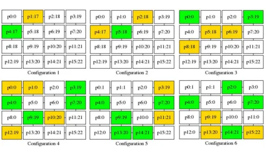
Self-stabilization of Algorithm1. Let p be any node. When the clock of p is at most nincrements behind the clock values of all its neighbors, p is enabled to increment its clock modulo K by Action I(p); see, e.g., node p4 in Configuration 5 of Figure1. In contrast, if the clock of p is not equal to 0 and p has a neighbor q such that p.c is more than n increments behind q.c and q.c more than n increments behind p.c, then p should reset its clock to 0 using Action R(p); see, e.g., node p1 in Configuration 1. The legiti-mate configurations of Algorithm1are those where for any two neighbors p and q, we have p.c ∈ {(q.c − 1) mod K, q.c, (q.c + 1) mod K}. Algorithm1is a self-stabilizing algorithm under the distributed daemon in the sense that starting from an arbitrary con-figuration, every asynchronous execution of Algorithm1eventually reaches a legitimate configuration from which every possible execution suffix satisfies the following
specifi-Fig. 1. Five steps of Algorithm1for K = 257 on a 16-node grid (fromSASA). "pi : j" means that pi.c = j. Enabled nodes are in orange and green. Moreover, orange nodes are activated within the next step.
cation: (1) in each configuration, the difference between clocks of every two neighbors is at most one (Safety); and (2) each clock is incremented infinitely often (Liveness). Time complexity units. Three main units are used for counting time: steps, moves, and rounds. Steps simply refer to atomic steps of the execution. A node moves when it executes an action in a step. Hence, several moves may occur in a step. Rounds capture the execution time according to the speed of the slowest node. The first round of an execution e is the minimal prefix e0 of e during which every node that is enabled in the first configuration of e either executes an action or becomes disabled (due to some neighbor actions) at least once. The second round of e starts from the last configuration of e0, and so on.
These notions are illustrated by Figure1. The second step (from Configuration 2 to 3) contains two moves (by p2 and p4). The first round ends in Configuration 3. In-deed, there are two enabled nodes, p1 and p4 in Configuration 1. Node p1 moves in the first step, however in Configuration 2, the round is not done since p4 has neither moved nor become disabled. The first round terminates after p4 has moved in the second step. Consequently, the second round starts in Configuration 3. This latter actually terminates in Configuration 6.
3
The
SASASimulator
3.1 SASAFeaturesThis Section surveys theSASAmain features. More information is available online as
Batch simulations. They are useful to perform simulation campaigns, e.g., to evaluate the average-case complexity of an algorithm on wide families of networks, including random graphs. They can also be used to study the influence on some parameters. Interactive graphical simulations. It is possible to run a simulation step by step, or round by round, forward or backward, while visualizing the network as well as the enabled and activated nodes; see snapshots in Figure1. New commands can be also programmed so that users can navigate through the simulation according to their spe-cific needs.
Predefined and custom daemons. The daemon, which parameterizes the simulation, can be configured. First, SASA provides several predefined daemons, including the synchronous, central, locally central, or distributed daemon; for such daemons, non-determinism is resolved uniformly at random. But, the user can also build its own cus-tom daemon: this is useful to experiment new activation heuristics, or explore worst cases. Indeed, the daemon can be interactively controlled using a graphical widget: at each step, the user selects the nodes to be activated among the enabled ones. The dae-mon can also be programmed; such a program can take advantage of the simulation history to guide the simulation into particular directions.
Test oracles. Expected (safety) properties of algorithms can be formalized and used as test oracles. Typically, they involve the number of steps, moves, or rounds that is necessary to reach a (user-defined) legitimate configuration. In order to define such properties, one has access to node state values and activation status [16]. Properties are checked on the fly at every simulation step.
3.2 The Core ofSASA
reads
loads
generates reads generates Dynamic Library
sasa Simulation Data Network Topology
Algorithm ocamlopt
[.cmxs files]
[bin] [.rif file] [.dot file]
[.ml files] [bin]
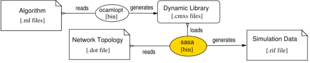
Fig. 2. TheSASACore Simulator Architecture
The core ofSASAis a stand-alone simulator; see Figure2. The user has to define both a network and a self-stabilizing algorithm following the API given in Section3.3. The algorithm is written as an OCAML program: the interface has been designed in such a way that theOCAMLprogram implementing the algorithm is as close as possi-ble to guarded commands, the usual way to write algorithms in the ASM. The network topology is specified using theDOTlanguage [12] for which many support exists such as visualization tools and graph editors. TheOCAMLalgorithm is compiled into a dy-namic library which is used, together with theDOTnetwork file, bySASAto generate
simulation data. A simulation data file contains an execution trace made of the sequence of configurations. That trace also contains the enabled and activated action history. Such traces can be visualized using chronogram viewers.
3.3 TheSASAAlgorithm Programming Interface
SASAalgorithms are defined using a simple programming interface specified in the 37 linesOCAMLfile, algo.mli, which is presented below.
Local States. Node states are defined by the polymorphic type ’st which can repre-sent any data the designer needs, e.g., integers, arrays, or structures. Nodes can access their neighbor states using the abstract type ’st neighbor (the "’st" part means that the type neighbor is parameterized by the type ’st). The access to neighboring states is made by Function state which takes a neighbor as input and returns its state; see Listing1.1.
type ’st neighbor
val state: ’st neighbor -> ’st
Listing 1.1. Access to neighbors’ states
Algorithms. To define an instance of the local algorithm of each node,SASArequires: 1. a list of action names;
2. an enable function, which encodes the guards of the algorithm; 3. a step function, that triggers an enabled action;
4. a state initialization function, used if no initial configuration is provided in theDOT
file. Indeed, even if self-stabilization does not require it, initialization is manda-tory to begin the simulation. For example, pseudo-random functions can be used to obtain an arbitrary initial configuration.
type action = string
type ’st enable_fun = ’st -> ’st neighbor list -> action list type ’st step_fun = ’st -> ’st neighbor list -> action -> ’st type ’st state_init_fun = int -> ’st
Listing 1.2. The step, enable, and initialization function types
The enable function takes the current state of the node and the list of its neighbors as arguments. It returns a list of enabled actions. The step function takes the same argu-ments plus the action to activate, and returns an updated state. The initial configuration can be set using an initialization function that takes as argument the node’s number of neighbors.
Topological Information. Algorithms usually depend on parameters relative to the network topology. For example, Algorithm1uses the number n of nodes. SASA pro-vides access to those parameters through various functions that the algorithms can use.
val card: unit -> int val diameter: unit -> int val min_degree : unit -> int val max_degree: unit -> int val is_connected : unit -> bool
Listing 1.3. Some of the topological parameters provided by the API
Example. Listing1.4shows the implementation of Algorithm1inSASA: notice that we obtain a faithful direct translation of Algorithm1.
open Algo
let n = Algo.card() let k = n * n + 1
let (init_state: int state_init_fun) = fun _ -> (Random.int k) let modulo x n = (* for it to return positive values *)
if x < 0 then n+x mod n else x mod n let behind pc qc = (modulo (qc-pc) k) <= n let (enable_f: int enable_fun) = fun c nl ->
if List.for_all (fun q -> behind c (state q)) nl then ["I(p)"] else
if List.exists (fun q -> not (behind c (state q)) && not (behind (state q) c)) nl && c <> 0
then ["R(p)"] else []
let (step_f: int step_fun) = fun c nl a -> match a with
| "I(p)" -> modulo (c + 1) k | "R(p)" -> 0
| _ -> assert false
let actions = Some ["I(p)"; "R(p)"]
Listing 1.4. Implementation of Algorithm1
3.4 Connection to the Synchrone Reactive Toolbox
In SASA, a simulation is made of steps executed in a loop. Each step consists of two successive stages. The first stage is made of the atomic and synchronous execution of all activated nodes (1-a), followed by the evaluation of which nodes are enabled in the next step (1-b).4At the second stage, a daemon nondeterministically chooses among the enabled nodes which ones should be activated at the next step (2). Overall, this can be viewed as a reactive program (Stage (1)) that runs in closed-loop with its environment (Stage (2)), where the outputs (resp. the inputs) of the program are the inputs (resp. the outputs) of its environment.
Thus, we could enlarge the functionalities offered bySASAby connecting our sim-ulator to the Synchrone Reactive Toolbox [19], which targets the development and val-idation of reactive programs. TheLUTINlanguage [23], which was designed to model stochastic reactive systems, is used to program daemons that take the feedback-loop into account. The synchronous languageLUSTRE[14] is used to formalize the expected properties. Indeed, this language is well-suited for the definition of such properties, as they involve the logical time history of node states. Such Lustre formalizations are used as oracles to automate the test decision [18]. Finally,RDBG[17], a programmable de-bugger for reactive programs, provides the ability to perform interactive simulations, visualize the network, and implement user tailored features.
4
Experimental Results
To validate the tool, we have implemented and tested classical algorithms using var-ious assumptions on the daemon and topology. Below, we give our methodology and some results.
Algorithms under test. We have implemented the following self-stabilizing algo-rithms: a token circulation for rooted unidirectional rings assuming a distributed dae-mon (DTR [8]); a breadth first search spanning tree construction for rooted networks assuming a distributed daemon (BFS [2]); a depth first search spanning tree construc-tion for rooted networks assuming a distributed daemon (DFS [6]); a coloring algorithm for anonymous networks assuming a locally central daemon (COL [13]); a synchronous unison for anonymous networks assuming a synchronous daemon (SYN [3]); and Al-gorithm1(ASY [7]). All these algorithms can be found in theSASAgitlab repository.2
Methodology. For each algorithm of the above list, we have written a direct imple-mentation of the original guarded-command algorithm. Such impleimple-mentations include the running assumptions, e.g., the topology and daemon. Then, we have used the inter-active graphical feature of SASAthrough the debuggerRDBG to test and debug them on well-chosen small corner-case topologies. Finally, we have implemented test ora-cles to check known properties of these algorithms, including correctness from (resp. convergence to) a legitimate configuration, as well as bounds on their stabilization time in moves, steps, and rounds, when available. Testing all those properties is a way to check the implementation of the algorithms. But, as these properties are well-known results, this is, above all, a mean to check whether the implementation ofSASAfits the computational model and its semantics.
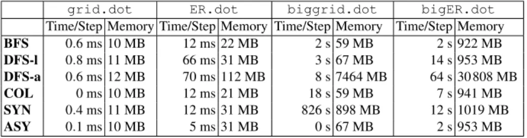
Performances. The results, given in Table 1, have been obtained on an Intel(R) Xeon(R) Gold 6 138 CPU at 2.00GHz with 50GB of RAM. We are interested in com-paring the performances of the simulator on the above algorithms, according to different topologies. Note that every algorithm assumes an arbitrary topology, except DTR which requires a ring network. Hence we perform measurements on every algorithm, except DTR. We have ran simulations on several kinds of topologies: two square grids, noted grid.dotand biggrid.dot, of 100 nodes (180 links) and 10 000 nodes (19 800 links), respectively; as well as two random graphs, noted ER.dot and bigER.dot, built using the Erdös-Rényi model [10] with 256 nodes (9 811 links, average degree
76) and 2 000 nodes (600 253 links, average degree 600), respectively. Every simula-tion, launched automatically, lasts up to 10 000 steps, except for the two big graphs (biggrid.dot and bigER.dot). For these latter, we have only performed 10 steps. For fair evaluation, we provide the execution time elapsed per step (Time/Step). Note that the DFS algorithm has been implemented using two different data structures to en-code the local states, namely lists and arrays. This leads to different performances; see DFS-l for list implementation and DFS-a for array implementation.
grid.dot ER.dot biggrid.dot bigER.dot Time/Step Memory Time/Step Memory Time/Step Memory Time/Step Memory BFS 0.6 ms 10 MB 12 ms 22 MB 2 s 59 MB 2 s 922 MB DFS-l 0.8 ms 11 MB 66 ms 31 MB 3 s 67 MB 14 s 953 MB DFS-a 0.6 ms 12 MB 70 ms 112 MB 8 s 7464 MB 64 s 30 808 MB COL 0 ms 10 MB 12 ms 21 MB 18 s 59 MB 7 s 941 MB SYN 0.4 ms 11 MB 12 ms 31 MB 826 s 898 MB 12 s 1019 MB ASY 0.1 ms 10 MB 5 ms 31 MB 0 s 67 MB 2 s 953 MB Table 1. Performance evaluation ofSASAon the benchmark algorithms. Time elapsing is mea-sured in user+system time in seconds or milliseconds, and has been divided by the number of simulation steps. Memory consumption is given in MegaBytes, and has been obtained using the “Maximum resident set size” given by the GNU time utility.
The results in Table1 show that SASA can handle dense networks of huge size. Hence, it allows to measure the evolution of time complexity of algorithms using a wide size variety of networks. Note that every simulation has been performed without data file (.rif, see Figure2) generation. Indeed, for large networks, this would pro-duce huge files and the simulator would use most of its time writing the data file. For example, a 10 000 steps simulation of DFS-a on bigER.dot generates 2GB of data and takes several days (instead of 15 minutes). Indeed, 100 millions values are gener-ated at each step. For such examples, being able to generate inputs and check oracles on the fly is a real advantage.
5
Conclusion and Future Work
This article presents an open-source SimulAtor of Self-stabilizing Algorithms, called
SASA. Its programming interface is simple, yet rich enough to allow a direct encoding of any distributed algorithm written in the atomic-state model, the most commonly used model in the self-stabilizing area.
In order to limit the engineering effort,SASArelies on existing tools such as, the
OCAML programming environment to define the algorithms, DOT to define the net-works, and the Synchrone Reactive Toolbox [19] to carry out formal testing and inter-active simulations.
In the spirit of TLA+ [20], an interesting future work consists in connectingSASA
to tools enabling formal verification of self-stabilizing algorithms. By connectingSASA
verified on some particular networks. This would imply to provide aLUSTREversion of theOCAMLAPI to encode algorithms.
Furthermore,SASAcould be connected to the PADEC framework [1], which pro-vides libraries to develop mechanically checked proofs of self-stabilizing algorithms using the Coq proof assistant [4]. Since Coq is able to perform automaticOCAML
pro-gram extraction, we should be able to simulate the certified algorithms using the same source. During the certification process, it could be useful to perform simulations in order to guide the formalization into Coq theorems, or find flaws (e.g., into technical lemmas) early in the proof elaboration.
References
1. Karine Altisen, Pierre Corbineau, and Stéphane Devismes. A framework for certified self-stabilization. Logical Methods in Computer Science, 13(4), 2017.
2. Karine Altisen, Stéphane Devismes, Swan Dubois, and Franck Petit. Introduction to Dis-tributed Self-Stabilizing Algorithms, volume 8 of Synthesis Lectures on DisDis-tributed Comput-ing Theory. Morgan & Claypool Publishers, 2019.
3. Anish Arora, Shlomi Dolev, and Mohamed G. Gouda. Maintaining digital clocks in step. Parallel Processing Letters, 1:11–18, 1991.
4. Yves Bertot and Pierre Castéran. Interactive Theorem Proving and Program Development -Coq’Art: The Calculus of Inductive Constructions. Texts in Theoretical Computer Science. An EATCS Series. Springer, 2004.
5. Adrien Champion, Alain Mebsout, Christoph Sticksel, and Cesare Tinelli. The kind 2 model checker. In Swarat Chaudhuri and Azadeh Farzan, editors, Computer Aided Verification, pages 510–517, Cham, 2016. Springer International Publishing.
6. Zeev Collin and Shlomi Dolev. Self-stabilizing depth-first search. Inf. Process. Lett., 49(6):297–301, 1994.
7. Jean-Michel Couvreur, Nissim Francez, and Mohamed G. Gouda. Asynchronous unison (extended abstract). In Proceedings of the 12th International Conference on Distributed Computing Systems, pages 486–493, 1992.
8. Edsger W. Dijkstra. Self-stabilizing Systems in Spite of Distributed Control. Communica-tions of the ACM, 17(11):643–644, 1974.
9. Shlomi Dolev. Self-Stabilization. MIT Press, 2000.
10. Paul Erdös and Alfred Rényi. On random graphs I. Publicationes Mathematicae Debrecen, 6:290, 1959.
11. Mitchell Flatebo and Ajoy Kumar Datta. Simulation of self-stabilizing algorithms in dis-tributed systems. In Proceedings of the 25th Annual Simulation Symposium, pages 32–41. IEEE Computer Society, 1992.
12. Emden R. Gansner and Stephen C. North. An open graph visualization system and its appli-cations to software engineering. Softw. Pract. Exper., 30(11):1203–1233, 2000.
13. Maria Gradinariu and Sébastien Tixeuil. Self-stabilizing vertex coloration and arbitrary graphs. In Franck Butelle, editor, Procedings of the 4th International Conference on Princi-ples of Distributed Systems (OPODIS), Studia Informatica Universalis, pages 55–70, 2000. 14. N. Halbwachs, P. Caspi, P. Raymond, and D. Pilaud. The synchronous data flow
program-ming language Lustre. Proceedings of the IEEE, 79(9):1305–1320, 1991.
15. Oded Har-Tal. A simulator for self-stabilizing distributed algorithms.https://www.cs. bgu.ac.il/~projects/projects/odedha/html/, 2000. Distributed Computing Group at ETH Zurich.
16. Erwan Jahier. Verimag Tools Tutorials: Tutorials related toSASA. https://verimag. gricad-pages.univ-grenoble-alpes.fr/vtt/tags/sasa/.
17. Erwan Jahier. RDBG: a Reactive Programs Extensible Debugger. In International Workshop on Software and Compilers for Embedded Systems, 2016.
18. Erwan Jahier, Nicolas Halbwachs, and Pascal Raymond. Engineering functional require-ments of reactive systems using synchronous languages. In International Symposium on Industrial Embedded Systems, 2013.
19. Erwan Jahier and Pascal Raymond. The synchrone reactive tool box. http:// www-verimag.imag.fr/DIST-TOOLS/SYNCHRONE/reactive-toolbox. 20. Leslie Lamport. Specifying Systems: The TLA+ Language and Tools for Hardware and
Software Engineers. Addison-Wesley Longman Publishing Co., Inc., USA, 2002.
21. Nils Müllner, Abhishek Dhama, and Oliver E. Theel. Derivation of fault tolerance measures of self-stabilizing algorithms by simulation. In Proceedings of the 41st Annual Simulation Symposium, pages 183–192. IEEE Computer Society, 2008.
22. Chritophe Ratel, Nicolas, and Pascal Raymond. Programming and verifying critical systems by means of the synchronous data-flow programming language Lustre. In ACM-SIGSOFT’91 Conference on Software for Critical Systems, New Orleans, December 1991.
23. Pascal Raymond, Yvan Roux, and Erwan Jahier. Lutin: a language for specifying and exe-cuting reactive scenarios. EURASIP Journal on Embedded Systems, 2008.
24. Kishor S. Trivedi. Probability and Statistics with Reliability, Queuing and Computer Science Applications, Second Edition. Wiley, 2002.
A
Artifact
We have set up a zenodo entry that contains the necessary materials to reproduce the results given in this article:https://doi.org/10.5281/zenodo.3753012. This entry contains:
– a zip file containing an artifact based on the (public) TAP 2020 Virtual Machine (https://doi.org/10.5281/zenodo.3751283). It is the artefact that has been validated by the TAP 2020 evaluation committee.
– a zip file made out of a public git repository containing the same set of scripts; the differences are that it is much smaller, and that the top-level script uses docker to replay the experiments. The entry also contains a link to this git repository. – a zip file containing the raw data produced by the experiment scripts via a Gitlab
CI pipeline of the git repository.
In more details, the artefact contains instructions to install the necessary tools, to replay the interactive session described in Section2 of the present paper, and to au-tomatically generate the data contained in Table1of Section4. The objective of this artifact is only to let one reproduce the results. If you want to learn more about the toolset, we advice the reader to look at the documentation and tutorials online [16].