A comparative evaluation of two acoustic signal dereverberation techniques

A COMPARATIVE EVALUATION OF TWO ACOUSTIC SIGNAL DEREVERBERATION TECHNIQUES

by

James B. Gallemore

B.S. United States Naval Academy (1971)

SUBMITTED IN PARTIAL FULFILLMENT OF THE REQUIREMENTS FOR THE DEGREES OF

MASTER OF SCIENCE IN OCEAN ENGINEERING, MASTER OF SCIENCE IN ELECTRICAL ENGINEERING

and

ELECTRICAL ENGINEER at the

MASSACHUSETTS INSTITUTE OF TECHNOLOGY June 1976

Signature of Author. ... Department of Electi3cal Engineering and Computer

Science, May 7, 1976 Certified by....

Thesis Supervis 9 (Academic)

Accepted by.... _{• •} .0.

Chairman, Oce g eet e i p p artment Copmittee o

ra. u a" t ,dents. /I/ Accepted b .-..

Chairman, Electrical Engineering and Comjputer Science Department Committee on Graduate Students

ARCHIVES

JUL 21

1976

A COMPARATIVE EVALUATION OF TWO ACOUSTIC SIGNAL DEREVERBERATION TECHNIQUES

by

James B. Gallemore

Submitted to the Departments of Ocean Engineering and Electrical Engineering and Computer Science on May 7, 1976 in partial

fulfillment of the requirements for the Degrees of Master of *I Science in Ocean Engineering, Master of Science in Electrical

Engineering and Electrical Engineer.

ABSTRACT

Two dereverberation techniques are applied to synthetic seismic data and their performance in removing water column multiples is evaluated and compared. One method is an applica-tion of homomorphic deconvoluapplica-tion and the other utilizes

linear estimation based on a minimum mean square error criterion. * The analytical formulations of both methods are discussed.

Performance is evaluated in terms of three criteria: percent of multiple energy removed, percent of signal (reflector) distortion, and visual improvement of the data. Results are presented which represent the performance of both algorithms for a range of environmental and signal processing parameters * including white noise level, multiple coherence, reflector/

multiple overlap, filter parameters and water column travel time estimate. The techniques are found to have comparable effectiveness on the synthetic data; however, indications are that homomorphic dereverberation has greater potential in shallow water applications while the linear technique appears to be more efficient for deep water data.

THESIS SUPERVISOR: Arthur B. Baggeroer

* TITLE: Associate Professor of Electrical Engineering and Associate Professor of Ocean Engineering

-2-ACKNOWLEDGEMENTS

The assistance I have received from several of my friends has been generously given and is very gratefully appreciated.

I would especially like to thank Professor Arthur

Baggeroer for guiding me toward an interesting topic and freely sharing his knowledge and experience throughout this endeavor.

Ken Theriault has helped me from the beginning of this

project in more ways than I can name. His advice and encourage-ment have contributed tangibly to the quality of my work and the enjoyment I have derived from it.

I would not have completed the homomorphic analysis with-out the frequent assistance of Jose Tribolet, who supplied me with his phase unwrapping algorithm and several of his other computational routines. He has also shared much of his time with me in tutorials and discussions which I have enjoyed and

appreciated.

Ken Prada, Tom O'Brien and Steve Leverette of the Woods Hole Oceanographic Institution have assisted me in learning to use the data processing equipment and allowed me time in their busy computer schedule to complete this project. I appreciate their support and cooperation very much.

I would like to thank my fellow students, Dick Kline and Tom Marzetta, for their frequent advice and discussions and moral support.

TABLE OF CONTENTS CHAPTE R I

CHAPTER II

CHAPTER III CHAPTER IV

INTRODUCTION AND PROBLEM STATEMENT... ANALYTICAL FORMULATION AND IMPLEMENTATION ... A. Analytical Formulation of the TDL Filter... B. Implementation of the TDL Algorithm ... C. Analytical Formulation of Homomorphic

Deconvolution ...

D. Implementation of Homomorphic Deconvolution... DESCRIPTION OF THE PERFORMANCE ANALYSIS... RESULTS ... A. Introduction ...

B. Results of TDL Dereverberation Performance .... 5 13 13 23 26 37 42 52 52 53 i. Operator Length, Multiple Distortion

and Multiple-to-Signal Ratio... 53

2. Water Travel Time Estimate ... 68

3. Multiple Periodicity... 77

4. Reflector/Multiple Overlap... 81

5. Additive White Noise and Filtering... 89

C. Results of Homomorphic Dereverberation Performance ... 102

1. Introduction... 02

2. Multiple Periodicity ... 103

3. Multiple-to-Signal Ratio... J08 4. Multiple Distortion ... 10

5. Water Travel Time Estimate ... 15

6. Reflector/Multiple Overlap... 17

-4-D. Comparative Examples of Processing Results ... .143 CHAPTER V SUMMARY AND DISCUSSION ...155 REFERENCES ... 162 APPENDIX A COMPUTATION OF THE PHASE DERIVATIVE OF THE

CHAPTER I

INTRODUCTION AND PROBLEM STATEMENT

The geologic structure of the earth beneath the seafloor is most often determined by seismic profiling. The procedure generally involves excitation of an impulsive acoustic source near the sea surface and recording of the reflected earth

response with a hydrophone array. Low frequency sound penetrates the bottom and propagates in the substrata with reflections occurring at discontinuities in the acoustic

impedance of the earth. The thickness and density of sub-bottom layers may be estimated from the reflected acoustic

signal, or seismogram.

The earth is modelled as a discrete layered medium with distinct interfaces for most seismic applications. This assumed structure, while not strictly accurate, has led to good processing results in practical seismic work and has the

additional advantage of being analytically tractable. We shall employ this assumption throughout the present analysis. A

detailed description of the earth model used is given in Chapter III.

The amount of energy reflected at a discontinuity is ideally measured by the reflection coefficient,

r2c₂ - rc₁c r2c_{2 + r1c}

-6-where rl, r2 and cl, c2 are the densities and acoustic

velocities in media 1 and 2. Here the sound propagates from medium 1 to medium 2 and normal incidence has been assumed. The assumption of normally incident plane waves is generally made in single channel (one receiver) seismology since it leads to analytical simplicity and appears to be reasonably accurate. In utilizing this simplified model we have ignored near field effects and spreading losses. These are not of major importance in single channel dereverberation and their inclusion would unnecessarily complicate the earth model.

It is evident from the reflection coefficient expression that large reflections occur at points of significant change in impedance. The largest impedance discontinuity encountered by seismic signals occurs at the water-air interface where R is nearly -1. The water-bottom interface is also a strong reflector in most cases. Thus, the water column becomes a reverberating channel wherein a significant portion of the

source energy is trapped. Repeated reflections from the bottom, or multiples, are received at intervals corresponding to the

two-way travel time of sound in the water column. Deeper reflections from the substrata are masked by multiples when their arrivals are nearly coincident in time. Since propaga-tion losses are much smaller in water, the energy in the

multiples is usually large compared to that in the deeper reflectors. Thus, water column multiples form an unwanted

component of the seismogram.

The reflection coefficient expression indicates that

all earth layers also introduce reverberation. Except in some shallow water situations, internal multiples are generally not a serious problem for two major reasons. Most importantly the acoustic attenuation in the earth is much greater than that in water so that very little internal multiple energy

is actually returned to the receiver. Secondly, the reflection coefficients at earth layer boundaries are usually small

compared to those at the surface and seafloor so that a relatively small part of the incident energy is actually trapped.

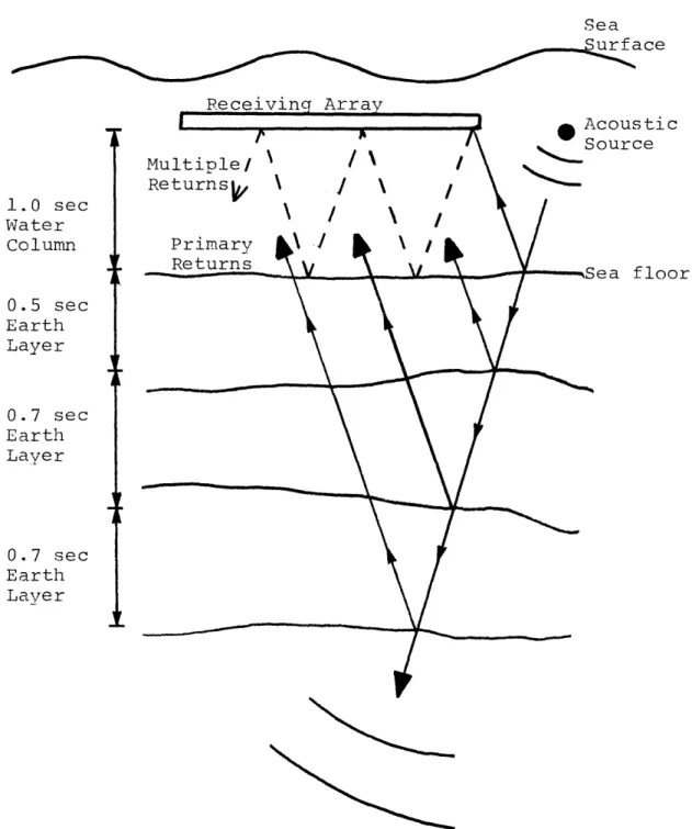
Figure 1 shows a synthetic seismogram with strong multiples. Response amplitude is measured on the ordinate and travel time in seconds on the abscissa. The first large

signal component is the bottom reflection at one second of travel time or about 750 meters water depth. The first multiple is an attenuated, phase-inverted replica of this

reflection at two seconds. Note that the return from a

reflection horizon at two seconds travel time would coincide with this multiple and be obscured. The overall periodicity of the multiples is apparent in this plot. Actual reflectors occur at 1.5, 2.2 and 2.9 seconds. Figure 2 shows the seismic

environment which would produce such a seismogram.

1st Sub-bottom Reflector R1 Bottom Response

k

1.0 1st M1ltipDl Bl 2nd Reflector R2 3rd Reflector R3 2nd Mu11 ti lc 3rd Muil iD 1 e B2 B3 ii1 . 2.0 3 3.0 4.0

Travel Tinme (sec)

Figure 1 Synthetic seismogram including three multiples. Reflectors are designated

Ri and multiples by Bi.

I 0.0 .0 I I - - - -i -i ,I r· r·

1

_{ii ja}

r~~'--~-~--Sea urface 1.0 sec Water Column 0.5 sec Earth Layer 0.7 sec Earth Layer 0.7 sec Earth Layer ustic rce floor

Figure 2 Earth structure like that shown

which would produce seismogram in Figure 1.

-10-algorithm was proposed by Backus [1]. His approach was to characterize the water column as a sharp, ringing filter with an impulse response composed of a weighted sum of delayed

impulses. The weights and delays are determined by the bottom reflection coefficient and the water column travel time

respectively. This model leads to a three-point operator with elements spaced at intervals corresponding to the two-way

water travel time. Implementation of the Backus filter requires estimation of the bottom reflection coefficient and water

column travel time. Several aspects of the performance of this method are discussed in Chapter II.

Spatial processing has also been used to reduce

multiples [2]. Spatial schemes normally require multichannel arrays of large physical extent which can be effectively focused to discriminate against reverberation. Such systems are widely used and quite effective in shallow water but their costs, both for hardware and data processing, are very high. Hence, there is still a need for time domain multiple removal techniques in deep water situations and for single channel systems.

Two techniques have recently been applied to seismic multiple removal with demonstrated success. The first, an

inverse filter algorithm based on a tapped delay line model, is due to Baggeroer [3], and is referred to hereafter as the TDL

filter. A tapped delay line is simply a realization of the time domain convolution of a sicnal and a gapped operator [4].

Results of this method have proven superior to those of three-point filtering, at least in some deep water situations.

A nonlinear filtering scheme using homomorphic deconvolu-tion has been applied to several aspects of seismic signal processing. The use of this method for dereverberation has

been demonstrated by Stoffa, Buhl and Bryan'5]. The homomorphic transformation is essentially a mapping from convolution to addition so that, after transforming, deconvolution can be accomplished by simple linear filtering. Seismic dereverbera-tion appears theoretically to be a very promising applicadereverbera-tion of homomorphic deconvolution because of the distinct properties

of seismic signal components. The method has not, however, been fully evaluated or widely used in practice.

The motivation for this study arises from the disparate theoretical mechanisms by which these techniques operate to perform the same function. Since analytical comparison is

not feasible, this functional, comparative approach is thought to be the best means of gaining insight into this interesting problem.

The purpose of the analysis is twofold. First, it is intended to indicate those factors which have significant effects on the performance of each algorithm. The factors to be considered are environmental variables and processing parameters. These are discussed in Chapter III. Secondly, the analysis is intended to point out the relative strengths

-12-and weaknesses of the methods by comparison of results on similar data.

Each algorithm is evaluated for a range of simulated processing conditions. Quantitative and qualitative criteria are specified which provide a comprehensive description of the manner in which each signal is affected by processing for multiple removal. These criteria also serve as a basis for comparison of results. The scope of the analysis and the specific performance criteria are discussed thoroughly in Chapter III.

CHAPTER II

ANALYTICAL FORMULATION AND IMPLEMENTATION

A. Analytical Formulation of the TDL Filter

A simple feedback model for the propagation of reverberat-ing seismic signals is given by Baggeroer [3]. Multiple

removal based on this model is then formulated as an inverse filtering problem. The dereverberation filter is designed using a least squared error criterion and the constraint that the filter have a tapped delay line structure.

The formulation will be developed here from a different point of view using Baggeroer's feedback model as a starting point. A summary of the feedback model is included for clarity.

Figure 3 shows the Laplace transform representation of a propagating seismic signal. S(s) is the transform of the

source signature. The signal first encounters the downward travel time delay which corresponds to a phase shift in this domain. Hb(s) represents the transfer function of the earth beneath the water column including the reflections from layer boundaries which comprise the desired information. Internal multiples or reverberations between the various earth layers are also included in Hb(s). Another phase shift corresponds the return of the reflected signal through the water column. P(s) is the feedback gain representing the water column multiple mechanism. In most cases this is well approximated by -1,

I S 0 0 0 0 0

S (s)

Figure 3 Laplace transform model of propagating seismic signal

Ro (s)

RgS

0 ₀

reflection at the surface. H (s) includes the observation effects such as hydrophone bandwidth and array tow depth. Ambient noise and reciever front end noise are modelled as additive white Gaussian noise.

The overall transfer function is -2sT R (s) H (s) Hb(s) e w S(s) 1 - P(s) Hb(s) e-2 wW

where T is the one-way water travel time and R (s) is the received signal without additive noise.

It is apparent that the presence of multiples is due only to the denominator of this expression. Thusfar we have

assumed implicitly that the earth response can be modelled accurately as a linear system and that the multiples are exactly periodic. The validity of these assumptions will

become apparent in the discussion of performance in Chapter IV. The obvious task is now to design an inverse filter having the form

-2sT F(s) = [1 - P(s) Hb(s) e w

Hence, we are required to estimate Tw and the impulse response, hb(t), corresponding to Hb(s). The earth response need not be estimated precisely for its entire duration. Estimating the dominant energy part of hb(t) is adequate to produce an effective dereverberation filter. A typical deep water

-16-seismogram has the great majority of its energy concentrated in the first 200-300 msec of its duration. Effective represent-ation of this portion of the signal requires about 10-20

filter coefficients, depending on the bottom and source characteristics.

The transfer function of eauation (1) can be re-written in series form as

R

(s)

ca

(s)

_(n=l)

S(s) n=1 -2nsT n+l w (-1) Hb(s) e .

The received signal then has the time domain representation

o0

r (t) = s[ho(* 0(t) * I (-1) hb(t - 2nT )] n=l

where * represents convolution. This can be rewritten as the sum of the primary return and the multiple signal.

r (t) = s(t) * h (t) *h (t- 2T ) + (-l)n+lh (t-2nT )

o( I t n=2 (

r (t) = b(t) + m(t) where

b(t) = s(t) * h (t) * hb(t-2T ) is the received primary and

00

Mr(t) = s(t) * h (t) * C hb(t-2_nTw)

is the received multiple signal.

The estimation problem, given the feedback model of figure 3, is to determine b(t) in the presence of rm(t) and white noise, w(t). It is convenient to group the unwanted

iAignal components.

n(t) = m(t) + w(t) (2)

Since the unwanted component is an additive one, we can consider estimating n(t) and subtracting the result from the received signal. We then have the filtering prohlem depicted in figure 4.

r(t) = b(t) + n(

b(t)

Figure 4

Here f(t) is the filter impulse response and n(t) is the minimum mean square error (MMSE) estimate o:f n(t), given the received signal r(t).

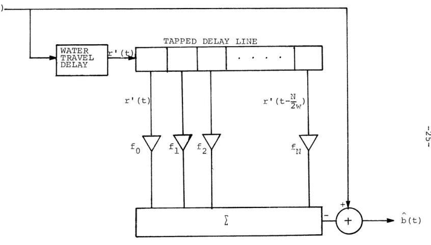
The number of digital filter coefficients to be estimated is 2TW+1, where T is the effective duration (portion contain-ing about 80% or more of the signal energy) of Ih,(t) and W is the signal bandwidth. The coefficients will then be spaced at the Nyquist sampling interval of 1/2W seconds.

-13-The optimum digital filter for n(t) will have coefficients, f which minimize 1

_f

e =E n (i/2W) -ni2)2 i=i _-J (3a) Lwhe ZE: n (i/2W) = I k=i _O fk rL (i-k) 2

The input in (3b) is shifted by the two-way travel time to avoid useless filtering of the signal prior to the bottom reflection.

[i /2W, if/2W] is the time interval over which n(t) is observed. Substituting (3b) into (3a) yields

S}

e = E fk (i-k) 2T - n(i/2W) . O O Minimizing, e I (i-k) -n(i(i-k) SE 12 fk r 2W 2_{T -n(i/2W)} r 2W - 2T

if

=i-

-O f

=

fk R (i-k)/2W k=i _o k rr - Rnr (k/2W+2T ).nr w

Here we have assumed stationarity over the duration of the

multiple period. This assumption has led to effective process-ing of both real and synthetic data. From (2)

Rr (k/2W+2T_nr w_w ) = R _mr (k/2W+2Tw ) _w + R _wr (k/2W+2Tw )_w

(3b)

(4)

A

--Here it is useful to assume (see ref.E3], p.15) that for shifts close to 2T the cross-correlation of w(t) and r(t) is very

w

small compared to R (T) which will generally have a peak in mr

this region. This is equivalent to assuming that the white

noise has a very short correlation time compared to 2T . We then have Rnr (k/2W+2Tw ) Rmr (k/2W+2Tw ) so that (4) becomes if fk R rr((i-k)/2W) = Rmr(k/2W+2T ) (4a) k=i

Baggeroer has derived equation (4a) by designing the

Wiener filter for b(t) with the constraint that the filter have a tapped delay line structure, i.e.

2TW

f(t) = 6(t) - X fk 6(t-k/2W-2T ) (5) k=o

When our estimate, n(t), is subtracted from the unshifted, received signal, the resulting overall filter operation has exactly the form of (5). This indirect approach yields the estimator equations of reference [3] without imposing the TDL structure directly.

The above derivation also emphasizes the estimator-subtractor or prediction error structure of this filter. The entire impulse response may be written as follows:

-20-i, 0, O _{.... 0, -fl' -f2'" "-fk} 2T zeros

w

This is the prediction error structure for a prediction distance of 2T _w. Equation (4a), however, which generates the {fi .}

differs from the prediction equations in that the right hand side vector is R mr(T+2T w) rather than R rr(T+2T w). As written, equation (4a) corresponds to the Wiener filter which produces the MMSE estimate of m(t) with r(t- 2Tw) as an input. Subtraction of this estimate from r(t) whitens only those spectral compon-ents which are due to the multiple.

It is simply proved that the magnitude of the error in b(t) is equal to that in the prediction operator.

b(t) = r(t) - n(t)

b(t) = b(t) + (n(t)-n(t))

A A

lb(t)-b(t) = In(t)-n(t)

Thusfar the only departures from optimum estimation have been the two assumptions of stationarity and the relative insignificance of R _wr (T+2T ). _w One further assumption is required for actual implementation of the filter. Note that Rmr(T+2T_{w )} is a required input which is apparently not measur-able from the given data. Baggeroer has observed that for the deep water case, which is of primary interest for this method,

Rmr (T+2Tw)ý: R rr (T+2T) .

That is, for shifts of nearly twice the water travel time, the great majority of the crosscorrelation energy is due to m(t). Hence, the equations used for data processing are given by

f

k fk Rrr((j-k)/2W) = Rrr (j/2W+2Tw) j=0,1,...2TW

k=i

Having seen the analytical formulation of this inverse filtering procedure it is instructive to compare it with the Backus three-point method. Processing actual data with both

filters (ref.[31]) has shown the Backus filter to be significantly less effective. Some reasons for this are apparent from the

foregoing analysis.

The Backus filter is rigidly dependent on the accuracy of two assumptions. The first, the assumption of strictly periodic multiples, is violated due to the horizontal separation of

source and receiver. This effect becomes more severe as water depth decreases. Since the Backus filter is implemented as

only three, equidistant operator coefficients it is very sensitive to this lack of periodicity. Even if the statistics of the

signal generate very accurate estimates of the bottom reflec-tion coefficient the filter structure is so simple and rigid

that proper cancellation will not occur if the multiples are significantly aperiodic.

-22-A second restrictive assumption of the Backus filter is that the bottom reflection should be accurately characterized by a single reflection coefficient. All of the statistical information available is forced into a single parameter estimation scheme. It is apparent that such a filter lacks

flexibility for dealing with more complicated bottom interaction mechanisms.

The relatively better performance of the TDL filter on real data is apparently due to its greater inherent flexibility. That is, the finite length impulse response, or prediction

operator, gives the filter a capability for removing reverbera-tion effectively in cases where the bottom response is not

accurately modelled as a weighted impulse. If the bottom has a ringing or smearing effect on the incident signal then the deconvolution operator must be extended in time. The Backus

filter, because of its rigid structure, cannot accomodate these situations. The TDL structure provides 2TW+l (usually 10-20) parameters which can be varied in the design procedure to optimize dereverberation of each seismogram. The special case of an ideal bottom will generate a filter response which is

essentially a single spike proportional to the bottom reflection coefficient. This result has been confirmed in the analysis of

synthetic data. In such a case the TDL filter consists basically of the first two points of the Backus three-point

was found to be essentially independent of operator length. The structural flexibility of the TDL filter also gives it some potential for dealing with aperiodic multiples. It should be noted, however, that the TDL algorithm, like the Backus and other classical dereverberation techniques, is

essentially a correlation-cancellation operation. Consequently, increased aperiodicity of multiples can be expected to degrade performance in all cases.

B. Implementation of the TDL Algorithm

Figure 5 shows a flow diagram of the filter implementation used for this analysis. Actual programming was done in

Fortran IV for use on a 32K computer. Referring to figure 5, the correlation function is computed by the standard shift-and-add operation with no windowing applied. Results of windowing

are included in reference [3]. Correlation time is variable and may be specified by the operator. The crosscorrelation

function is approximated by the correlation function as discussed in the previous section.

Solution of the filter equations is accomplished by conventional matrix inversion. The Toeplitz symmetry can be exploited for computational savings. Spacing of the operator elements is determined by the estimated signal bandwidth which

is specified as an input parameter.

-24-RECEIVED SIGNAL

DE REVE RBE RATED

SIGNAL

Figure 5 Flow chart of TDL algorithm. CORRELATION FCN

R (T)

_rr APPROXIMATE CROSS CORRELATION FCN R _{(T+2T )} mr w SOLUTION OF ESTIMATOR EQUATIONS

SfiR rr(Ti)=Rmr (T.i+2Tw)_{i rr i mr 1 w}

IMPLEMENT TDL b(t)=r(t) *{f } 1 I I

-b(t)

-26-figure 6, i.e., by means of a tapped delay line or, equivalently, convolution with the gapped operator.

C. Analytical Formulation of Homomorphic Deconvolution A homomorphic system is one which obeys a generalized principle of superposition and which can be represented as an algebraically linear transformation between two vector spaces. A detailed description of the theory of homomorphic systems is given by Oppenheim and Schafer [6]. This material will not be repeated in depth here; rather, we shall discuss the basic characteristics of homomorphic systems for convolution with emphasis on those properties which facilitate dereverberation. Additional discussions of these properties are found in

references [51, [71 and [8].

The usefulness of linear systems for separating additively combined signals is due primarily to superposition. Signals which are added and happen to be disjoint in the frequency domain can be separated by means of an appropriate bandpass filter. Homomorphic systems for convolution have a similar effect on signals which have been convolved. That is, a homomorphic transformation maps the input signal to a domain in which the convolved components may be disjoint. Such a transformation is illustrated in figure 7.

(n) _{xI(n) Z} .. 1X(z) _-

_-

FX(z)

_{log [-}

e-

_-

_{Z x (n)}^7

The mapping characteristic of this system is intuitively apparent. Suppose x(n) is composed of two components which have been convolved.

x(n)

=

x

1

(n)

* x

2

(n)

The z-transform operation yields a signal with multiplied components, X₁(z) and X₂(z). The logarithm output is

X(z) = log[X_l1 (z)] + log [X₂(z)]. The inverse z-transform,

x(n)

=

x

1

(n)

+

x

2

(n)

preserves the additive combination of the components and yields a sequence which is real and stable for a real and stable x(n). The sequence x(n) is called the complex cepstrum of x(n).

Although it is real for real inputs, the "complex" is retained to emphasize that it contains both the magnitude and phase

information from X(z). Hence the complex logarithm is required even for real x(n). (We shall omit the modifier here for

brevity.)

The cepstrum variable, n, is normally called the quefrency (a paraphrase of frequency) or period variable. Filter opera-tions in this domain are generally similar to those encountered in the frequency domain. Exact subtraction of xl(n) from x(n) followed by computation of the inverse cepstrum (figure 8) yields the sequence x₂(n), exactly, in the time domain.

-28-(n)-

X(z) X(z)(n)

x (n)

z

_'expl

]---

_Z

-1 -- x (n)

Figure 8

It is this property which renders homomorphic processing valu-able for deconvolution.

As an example of complex cepstrum transformation consider a signal composed of a short pulse (2 samples) convolved with a decaying, periodic impulse train.

x(n) = s(n) * p(n)

x(n) = (n) + 6(n+1)+ * ) (-1)kRk6(n-kT) k=o

where

IRI < 1 and T > 2 Taking the z-transform,

oo k k -kT X(z) = (1 + z/2)- I (-1) kR z k=O -1 -T X(z) = (1 + z/2).(l + Rz ) .

The logarithm then produces a sum

Both terms are simply expanded in Laurent series. log (1 + z/2) = -T log (1 + Rz - n n n n=-l n2 -n nn (-1) nR n=l n

,

jzj<

2

-nT _{IRzT < 1}

The z-transforms are easily recognized.

_-1)n

s(n)- -ln_-n n2 n (-1) kRk p (n) 6(n-n = -1, -2...-. -kT) , k = 1,2,..., x(n) = s(n) + p(n)

We see that s(n) occupies only the negative quefrency region and p(n) only the positive quefrency region. Exact deconvolution can be accomplished in this case by zeroing the desired half of the cepstrum.

The canonic form of homomorphic systems for convolution is shown in figure 9.

- - A

x (n) -

₁

D,

1 x(n) y(n)

j--

-1 y (n)

-30--1

The characteristic systems D, and D, are shown in figures 7 and 8 respectively. The system L is a conventional linear system. When L has a transfer function of 1, then x(n) is

-1

recovered exactly at the output of D, . The choice of L will determine the effectiveness of deconvolution for a given input sequence.

Two further specifications are required to ensure the validity and uniqueness of the transformation. The complex logarithm is a multivalued function with an infinite number of branches.

log[X(z)] = log X(z) +

j

(Arg[X(z)i 2Trk) for all k where Arg specifies the principal value of the phase. This ambiguity must be resolved while simultaneously satisfying the requirement that X(z) be a valid z-transform. Note that if x(n) is to be real and stable, X(z) must be conjugate symmetric and analytic in an annulus of the z-plane containing the unit circle. That is, the real and imaginary parts of X(z) must be continuous functions of z in the region including the unit circle. The imaginary part, arg[X(z)], can only be made continuous by "unwrapping" Arg[X(z)] in such a way that all

jumps of ± 27k are removed. This unique unwrapping leads to a unique, valid X(z) which transforms to a stable, real x(n). The requirement of a continuous phase curve poses some

section.

It is apparent from the foregoing description that

homomorphic systems have the potential for separating convolved signals. One might expect, however, by analogy with linear systems that deconvolution is most effective for signals with certain cepstral properties. This is, in fact, the case and, fortunately, seismic signal components are generally amenable to deconvolution. Recall that a seismogram is modelled as a convolution of a source signature and an impulsive reflector series. Reverberation appears as a minimum phase, periodic addition to the reflector series. Thus, we have

r0 (n) = p(n) * (b(n) + m(n))

where p(n) is the source signature, b(n) is the desired signal and m(n) is reverberation. Generalizations can be made concern-ing the cepstral properties of each component.

The source signature is, in general, a mixed phase, short duration time sequence. It is clear from the definition of the z-transform that any such finite sequence transforms to a

rational function of z with no poles except at the origin. In general

m

-P(z) = C z k (1-a.z ) H (l-b.z) lail, lbjl< 1

i=l j=1

The a. and b. represent zeros inside and outside the unit circle -k

-32-^ m -i

P(z) = log C + • log(l-aiz ) + log(l-b z)

i=l j=1 log C n=O n ^ m a. p(n) = I n>O i= n (6) i=l P bn n3 n<O j=l

Here it has been assumed that the linear phase term is removed before computation. p(n) is a two-sided sequence which is always of infinite duration but decays faster than 1/n. Hence, most of the cepstral energy is concentrated near the quefrency origin.

The reflector sequence is modelled as a train of randomly spaced impulses which may be mixed phase. Stoffa, Buhl and Bryan [5] give a general, but very complicated expression for the complex cepstrum of such a sequence. Some specific examples are given by Schafer [7]. The resulting cepstrum is an impulse train with impulses at the time domain impulse locations, at all their multiples, and at various other loca-tions, both positive and negative on the quefrency axis. Three important observations can be made.

The cepstrum of a minimum phase reflector train contains no contributions for negative quefrency. Consider the special case of equation (6) in which all the b. are zero. This

corresponds to all zeros being inside the unit circle, i.e., a minimum phase sequence. Note that p(n) and s(n) in the example

are minimum and maximum phase respectively, leading to causal and anticausal cepstra.

Secondly, it happens that no non-zero cepstral contributions occur between the origin (first impulse) and the location of

the second impulse in time, if the time series is minimum phase. Therefore, the cepstrum of a minimum phase impulse train, unlike that of a general sequence does not have its contributions

concentrated near the origin. The cepstrum of a minimum phase impulse train will always contain a gap equal to that between the first two time domain contributions.

Finally, we observe (see Schafer [7]) that a reflector

series can easily be made minimum phase by exponential weighting.

r'(n)

=

w

n

_r(n)

_jwl

_<

₁

k m

-k

-R' (z) = C z

c

l-(aiw)z 1-(bj/w) i=l

The value of w is chosen so that -1

b_{.w -} 1 > 1 for all b..

Weighting of the impulse train is effected by weighting of the entire signal since, if

-34-then

wns(n) = (wnp(n))*(wnb(n)).

Note that the reflector series may be made minimum phase without making the entire signal minimum phase. Very little weighting

is normally required in practice.

The remaining contribution to the seismic signal is reverbera-tion. This component is merely a special case of a minimum

phase impulse train in which the impulses are periodic. It is easily verified that if

m(n) = ý y(n)6(n-kn ) k=l

then

m(n) = y(n/n ).

The cepstrum is, therefore, periodic with the same period as the reverberation.

A useful property for deverberation is derived by Stoffa, et al.[5]. The derivation is summarized here because of its direct pertinence to seismic processing.

Consider a normalized multiple signal,

m(n) = ý (-1) R 6(n-i2T ) (7)

i=0

where R is the bottom reflection coefficient. Then, as we have seen

•o ii

m(n) = 6(n-2iT ).

Subtracting the firstj cepstral contributions and transforming, ^ _j

_(n)

_{= m(n)} ^ _- (-1) R _{6(n-2iT )} w i=1 S i -2iT

Mj(z)

=

Ji i=j+l 0 R -2iT Mj (z) = H exp [-- z w] . i=j+l i

Expanding in a power series

00 M R ik -2ikT M. (z) 1= H X _k

i=j+l k=O k!i

S(-Rz2T +k oo -2T 2j+k

M (Z) = 1 + (-Rz w (-Rz w)V

k-I j+k k=3 i=l 2(i+j)(j+k-i) "'

(8)

Comparing (7) and (8), the first j time domain multiples have been removed completely and the (j+l)st multiple is reduced by 1/(j+l). All succeeding multiples are also reduced. Thus, removal of only the first cepstrum multiple would remove the first time domain multiple and reduce the second by 1/2, the third by 1/3, etc..

Having seen the cepstral properties of each seismic signal component the advantages of homomorphic deconvolution are

apparent. The source signature and reflector series have their cepstral energy concentrated in different regions of the quefrency

-36-axis, thus facilitating removal of the source. The cepstral contributions of the reverberation occur at predictable locat-tions so that multiple removal is possible.

Due to the nature of the homomorphic transformation,

linear filtering of the cepstrum is not the normal convolution operation but a simple zeroing of the unwanted contributions. That is, the linear filter is generally frequency invariant rather than time or quefrency invariant. The name "quefrency" was adopted to reflect this reversal of the customary time and frequency filtering roles.

The foregoing analysis is based on assumptions similar to those employed in classical seismic processing. Namely,

we have assumed that the seismogram consists of a source signature convolved with distinct, impulsive reflectors and periodic multiples. It is difficult to predict the sensitivity of the overall processing scheme to these assumptions because of its complex analytical structure. Hence, various parameters have been varied in the performance analysis to obtain an

empirical measure of this sensitivity.

Finally, we note that the additive noise was not included in the analytical formulation of the homomorphic processing scheme. The algorithm is designed to separate convolved

components and, unfortunately, no effective processing gain is achieved over added noise. In practive, additive noise has been dealt with through classical bandpass filtering. This

performance analysis includes a description of the effects of additive noise on homomorphic deconvolution.

D. Implementation of Homomorphic Deconvolution

Figures 7, 8 and 9 show the sequence of operations required for homomorphic deconvolution. A processing scheme was designed to implement this algorithm in Fortran IV on a 32K digital

computer. A flow diagram of the scheme is shown in figure 10. Some aspects of the computation are noteworthy.

All z-transforms in the algorithm are implemented via FFT. Recall from the analytical formulations that z-transforms

involved in the processing of a real, stable sequence are

required to have regions of convergence which include the unit circle. The discrete Fourier transform is simply a sampling of the z-transform on the unit circle which, for properly

band-limited signals, is sufficient to specify the signal completely. Data sequences are normally padded with zeros to reduce cepstral

aliasing, e.g., 2048-point cepstra are computed for 1024-point seismograms. Since the cepstrum is always of infinite extent, a truncated version always results in some aliasing when

computation is not done recursively.

The major difficulty in computing an accurate cepstrum is the computation of a continuous phase curve. The data sequences are normally sampled at a rate based on the frequency content.

There is no assurance, however, that this sampling rate is adequate to uniquely specify X(z) = log[X(z)].

RECEIVED

SIGNAL x(n)

Co_I

XR(k

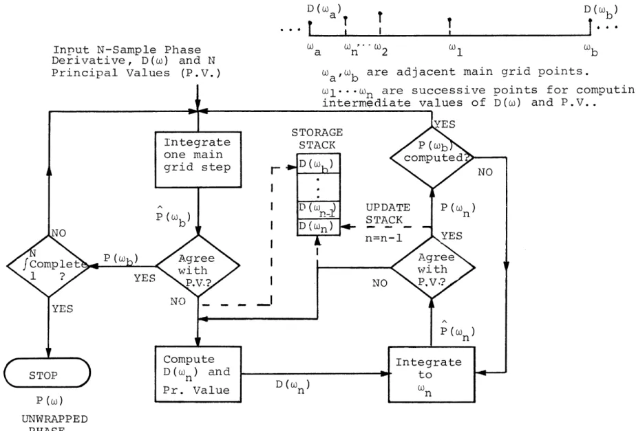
The method used for this analysis is due to Tribolet [9] and is thought to be quite accurate and efficient. The flow diagram for this algorithm is shown in figure 11.

dX z)

The phase derivative, dz and principal value, ArglX(z)], are easily computed from the transforms of x(n) and n x(n)

(see appendix A). The values of the derivative are integrated using the trapezoidal rule and the integral output is compared with Arg X(z) at each step. If the two values do not agree within

2n7 ±+ n = 0,+±, ±2,...

where E is a small positive number, the latest computed value of arg X(z), say ai , is discarded. The routine then returns

to the last correct integration value, computes an intermediate derivative value, and begins integrating with a step size half

that of the original grid. The integrate-and-compare process is continued at this step size until a. has been computed

1

correctly or until a comparisen fails. Integration is resumed at the initial step size in the former case or, in the latter, step size is again halved. The number of possible step sizes is theoretically unlimited. The value of c may be adjusted by trial-and-error for most efficient integration. The

adaptive step feature compensates for the undersampling problem in a very efficient and accurate manner.

Linear phase contributions are easily identified and removed from the computed continuous phase curve. Having

D(Wa

a T

r

I

Input N-Sample Phase Derivative, D(w) and N

Principal Values (P.V.)

a n 2

Wa, b are adjacent main grid points.

ints for computing w) and P.V..

UNWRAPPED PHASE

Figure 11 Flow chart of Tribolet phase unwrapping algorithm

D(w b)

computed the log magnitude and phase, the inverse z-transform is straightforward.

Linear filtering is accomplished by zeroing the unwanted cepstrum values. One might consider windowing procedures which are common in linear filtering, but these were not employed in the present analysis.

The inverse cepstrum computation is completely straight-forward since no ambiguities arise in the exponentiation

process. The final steps are shifting the output sequence

by the linear phase value and unweighting the shifted sequence, if necessary.

-42-CHAPTER III

DESCRIPTION OF THE PERFORMANCE ANALYSIS

The purpose of this analysis is to evaluate, both quantita-tively and qualitaquantita-tively, the performance of the TDL and homo-morphic dereverberation techniques. Each method is to be

evaluated for a variety of simulated seismic conditions in order to determine those factors which significantly influence perfor-mance. The comparative nature of the analysis is intended to

emphasize the relative strengths and weaknesses of each technique. It should be noted that absolute performance figures are

not inherently valuable, especially when obtained from synthetic data. The diverse geological and oceanographic conditions

encountered in marine seismology coupled with the many different processing systems currently employed may be expected to yield

a range of absolute results. The greater value of this analysis is to indicate the parameters, environmental and mathematical, which can be expected to affect significantly the performance

of these algorithms. The numbers obtained provide a measure of the relative performance of the two methods under similar conditions and, in some cases, provide asymptotic performance criteria. Synthetic data were chosen so that signal parameters could be accurately controlled.

Three criteria are specified for comprehensive evaluation of performance. The first, most direct, measure of effectiveness

is the percentage of multiple energy removed from the signal. This is easily measured by calculating the zero-lag correlation of the signal, in time windows spanning only the multiple

locations, before and after processing. That is, the squared amplitude (energy) of the signal in the multiple region is computed after processing and subtracted from the squared amplitude of the original signal in that region. This

difference is divided by the original energy of the multiple to yield the fraction of energy removed by processing. The use of synthetic data facilitates this method of analysis

since reflectors and multiples can be placed in disjoint regions to avoid ambiguity.

The second criterion is the amount of signal distortion introduced by dereverberation. This is measured by comparing reflector energy before and after processing. As before,

reflectors and multiples must be disjoint for meaningful results. Although these two criteria provide an accurate auantitative measure of performance they are restricted to situations in

which reflectors and multiples do not overlap. The overlap case is most important in processing real data since the

multiples then abscure the reflectors most severely. In order to judge performance in these situations we must evaluate

qualitatively the improvement of visual interpretability. This visual enhancement of reflector-to-multiple ratio is our third criterion. It is an important measure in spite of its

-44-subjective nature since the primary means of seismogram analysis is visual interpretation.

The analysis is limited in scope to the single channel processing configuration. Although both techniques are

applicable, in principle, to multichannel processing, the many additional variables involved and unavailability of appropriate synthetic data would lead to a complicated extension of this analysis. A single channel treatment is adequate to identify the important performance traits of both methods.

Parameters to be varied fall into two general categories; environmental and operational. The environomental parameters include noise level, multiple periodicity, multiple-to-signal level and multiple/reflector separation or overlap. These are varied within ranges which are thought to be representative of ambient conditions normally encountered in marine seismology. Effects of noise level are considered only for the case of white Gaussian noise. The effects of aperiodicity have not

been evaluated for the TDL algorithm because it is intended primarily for deep water use where only the first multiple is usually of interest. Operational parameters refer to those which can be controlled during processing. These include filter cutoff frequencies, operator lengths, travel time estimates, cepstral stopbands, and weighting. Windowing of the correlation function is not evaluated although a discussion of this subject is contained in reference 13].

The algorithm used in generating simulated earth impulse responses is due to Theriault 110]. A brief description of

Theriault's earth model is given here.

The model is based on the following assumptions:

(1) An air gun source generates longitudinal pressure

waves which impinge upon all earth layers as normally incident plane waves.

(2) _{All earth layers are horizontally infinite,} parallel and homogeneous.

(3) Abrupt changes in acoustic impedance occur at

each layer interface and these boundaries are characterized by the customary acoustic reflec-ion and transmissreflec-ion coefficients.

(4) The earth has a uniform density.

(5) The water column is a non-attenuating fluid with a perfect pressure release interface at its surface.

(6) Each layer is characterized by a transfer

function, F(w) which represents the attenuation

and travel time delay for that layer.

These assumptions are incorporated into a lumped parameter model. Figure 12 shows a frequency domain model of a two

layer earth. The Fi(w) have the functional form

exp -jwx i/(9)

-46-Hydrophone

Source

Figure 12 _{Two layer earth transfer function schematic} (after Theriault).

where xi, c_i and ai are the ith layer thickness, sound speed and layer attenuation parameter respectively. These transfer functions are combined using a semi-group property rather than the usual frequency domain multiplication.

The -1 multiplier completes a feedback loop around the source which generates the water column multiples. Since the water column is assumed to have no attenuation the multiples

appear in the earth response as impulses, and in the resulting seismogram as replicas of the source signature reduced by the bottom reflection coefficient.

The above multiple mechanism is inadequate for representing effects of incoherent (distorted) multiples and varying bottom interaction mechanisms. These effects are introduced by inser-tion of water column attenuainser-tion which causes the bottom response and multiple responses to be of exponential form given by the Fourier transform of (9). Thus the bottom response is extended in time and each multiple is a distorted version of the previous one. Examples of multiple appearance with and without water

column attenuation are shown in figure 13a and b.

The topmost loop of figure 12 simulates the effects of finite receiver depth T. Any number of layers with the desired parameters can be combined into an overall earth transfer

function which is easily transformed to yield the earth impulse response.

-48-B3 (a) (b) I I I I I I 1.0 2.0 3.0 4.0 5.0

Figure 13 (a) Synthetic seismogrimn wi th coherent multiples. (b) Synthetic seis.mogram ,'7ith distorted niultiples

convolution of various Theriault impulse responses with air gun signatures obtained from actual at-sea recordings. A typical signature is shown in figure 14.

It is important to note that these seismograms contain all water column multiples and internal multiples of all orders. For realistic parameter values earth attenuation characteristics usually render internal multiples negligible.

Finally, we note one drawback of using this model for multiple removal analysis. The algorithm produces multiples which are exactly periodic. This periodicity gives these

seismograms strong correlation characteristics which are not usually encountered in practice. The lack of periodicity in actual seismograms is due to the horizontal separation of the source and receiving array. The difference in travel paths arising from this separation is illustrated below for a primary return and first multiple.

surface

bottom 2d

primary path length -cos

_{cos a}

4d multiple path length

-50-0.0 0.25 0.50

Figure 14 Air gun signature (obtained by at-sea recordings) convolved with synthetic earth response functions to form seismograms.

For a known separation and water depth the travel time difference can be easily calculated. This effect becomes minimal in deep water where cos a and cos a are approximately equal to one.

-52-CHAPTER IV

RESULTS

A. Introduction

The results of applying the multiple removal methods

described in Chapter II to synthetic data are described here in terms of the criteria of Chapter III. Performance based on the first two criteria is emphasized because it can be quantified much more accurately. Specifically, the reflectors and

multiples have been positioned at distinct locations in most cases so that the amount of energy removed from reflectors and multiples can be measured without ambiguity. This emphasis leads, however, to a certain lack of realism in several of the synthetic data plots. Separation of this kind in an actual seismogram would, of course, eliminate the necessity for

multiple removal. Hence, several cases of interfering reflectors and multiples are also shown. Although these are not amenable to quantitative analysis they can be judged on the basis of the third criterion, viz., improvement of visual record quality.

A second deviation from normal processing conditions has been required to compare effectively the performance of the two methods. Homomorphic dereverberation is accomplished in practice (see [5]) concurrently with source deconvolution, where practical, since both operations are simply performed after the cepstrum has been computed. This leads to a

reflector location which is due to source deconvolution alone. Although this may lead to improvement of the record, the criterion

of energy removed does not accurately measure dereverberation performance in the same way it does for the TDL results. For example, source deconvolution might typically lead to 90% reduction of multiples and 90% removal of reflector energy. This gross change in configuration cannot be effectively compared with TDL processing on the basis of energy removed. Hence, source removal has not been accomplished in most cases

tested. The results of this "partial" processing can be

quantitatively evaluated and easily compared with TDL results. Cepstral filtering which includes source removal, thus retain-ing only high quefrency energy, is referred to as "longpass

filtering". Several examples of longpass filtering are included and interpreted in terms of the third criterion.

The performance of each method is discussed individually for various processing situations. A direct comparison of the performance of both methods for the same data is also included. The comparison is extended in Chapter V.

B. Results of TDL Dereverberation Performance

I. Operator Length, Multiple Distortion and Multiple-to-Signal Ratio

The number of tap gains required for optimum multiple removal was found to be highly signal-dependent. Recall from Chapter II that the tapped delay line is essentially an

-54-estimate of the high energy portion of hb (t), the earth impulse response. In most applications the reflected bottom response is dominant. The time-bandwidth product of this response

would then be expected to govern the filter length requirements. Measured results confirm this.

Seismograms containing exactly impulsive (one sample)

bottom responses exhibited little or no variation of performance with filter length. Typical filter impulse responses for a

seismogram of this type are shown in figure 15. The reflection coefficient in this case is 0.3. The first tap gain is close to -0.3 in each response, as would be expected from the Backus

formulation in which the second operator point is an estimate of the bottom reflection coefficient. Increasing filter length can be seen to cause variation in the "estimation" of the reflec-tion coefficient. Figure 16 shows energy removed vs. filter

length for this seismogram. Multiple energy removed decreases slightly with increasing filter length. Reflector distortion is nearly constant at low values (6% for one and -2% for the other). The signal used in figure 16 is shown in figure 17a. The processed result shown was obtained using only one tap.

Introduction of a non-impulsive multiple mechanism was found to produce a marked dependence of performance on operator length. Synthetic seismograms were generated with finite

length bottom responses, resulting in distorted multiples

-.32 -.31 -.28 I I V

/i

(

(b)

{"

V

/

(c)

Figure 15 TDL impulse responses for three operator lengths. (a) 5 taps (b) 10 taps (c) 15 taps

1st Multiple 3rd Multiple 2n MulAt-L ple

Reflectors

i i l 4 8 12 16 20 24 28 NUMBER OF TAPS

Figure 16 Operator length vs. performance for a signal with with impulsive multiples.

-56-J0UU 80 60 40 20 I I

-d1

1

I9 1 a I ,, I

R1 R2 B2 B3

1 i

II

(b) I I I I 1.0 2.0 3.0 4.0 5.0

Figure 17 (a) Seismogram with coherent multiples.

(b) Result of TDL processing with a one point operator.

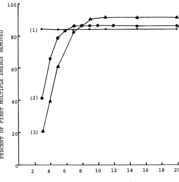
-58-Figure 18 shows filter performance vs. operator length for three seismograms having different degrees of distortion in their bottom reflection mechanisms. This distortion is

equivalent to extension of the bottom impulse response in time. The signals associated with curves (1), (2) and (3) are shown in figures 19a, 19b and 19c respectively. The increasing

distortion of the multiple at 2.0 seconds is evident. Curve (1) corresponds to a signal with very slight multiple distortion. Operator length is seen to have no effect on performance. The seismogram corresponding to curve (2) has a bottom impulse response which is significant for T = .03 seconds. The tap spacing in this case is 1/2W = 4.88 msec, so that 2TW = 6.1, and six or seven tap gains should be adequate if the signal has been properly sampled. Reference to curve (2) confirms that increasing the filter length beyond seven does not improve performance. Filters of fewer than seven elements yield

monotonically decreasing performance. The bottom response for curve (3) is significant for .045 seconds so that, for the same tap spacing, 2TW = 9.2 and we anticipate that nine or ten taps will he adequate. This is, in fact, the case.

Figure 20 shows the 5, 9 and 15 point filter impulse responses associated with curve (3). There is an observable

2 -bt

convergence to a t e shape which is the actual functional form of the synthetic bottom response. Figures 20a and 20b exhibit a "diverging tail" effect which was found to be common

100 80 60 20 (1) (2) )3 -\J / I I a I I I I I I I 4 6 8 10 12 14 16 18 20

TDL OPERATOR LENGTH (# OF TAPS)

Figure 18 Performance vs. operator length for three signals with bottom interaction times varying from (1) impulsive to (3) .045 seconds.

f% -

-W

-60-F^~---'

(a) (b) (c) I I 1.0 2.0 3.0 I 4.0 5.0

Figure 19 Seismngrars associated with the curves of figure 18. (a) Curve (1). (b) Curve (2). (c) Curve (3).

(a)

(b)

(c)

Figure 20 Filter impulse responses associated with Curve (3) of figure 18. (a) 5 points (b) 9 points

(c) 15 points.

I\

-62-when the specified filter length is too short. This type of phenomenon occurs in some numerical approximation methods when

an inadequate number of terms is specified.

It is apparent from the above results that the effect of operator length is closely related to the bottom interaction mechanism. As discussed in Chapter II, the filter should be an estimated replica of the bottom impulse response when the interaction process can be accurately modelled as a convolution of the source signature with the bottom response. Figures

15 and 20 are good examples of this behavior.

In the cases summarized in figure 18 performance increases as multiple distortion increases. This need not be true in general since bottom interactions may become very complex.

2 -bt

The slowly varying t e responses lead to operators which have a greater cancellation effect as they are extended. A higher bandwidth bottom impulse response might not exhibit

this behavior. As it was not possible to include more complicated bottom responses in the earth model used, these effects were not investigated further.

Reflector distortion was found to be nearly constant for all filter lengths tested. The reflector at 2.7 seconds was essentially undistorted in all cases. The 3.5 second reflector had an average distortion of 7%. Figures 21-24 show some

Bl

B2

B3

A

Fn----h~

(a) (b) 2.0

2.0

3.013 1 4.0 5 5.0

Figure 21 (a) Seismogram with very coherent multiples. (b) Result of TDL processing with three taps.

Fi

1.0

-64-

F----R1 R2

I

I

I

i

i

I

1.0 2.0 3.0 4.0 5.0

Figure 22 (a) Seismogram with moderately dittnrted m'ultiples; bottom response is significant for .035 seconds. (b) Result of processing with 7 taps.

R1 R2 B B B2 B

,I

1

(a)

1.0 2 2.0 i 3.0 4.0 5 5.0

Figure 23 _{(a) Seismogram with considerable multiple distortion;}

bottom response is significant for .045 seconds. (b) Result of TDL processing with 11 taps.

7 · 1

/Ijpj~~ i~v---c---.

-

-66-first three figures (21, 22 and 23) show signals before and after processing with the fewest number of taps required to achieve optimum performance. Visually, multiple removal is almost complete in each case. The signal of figure 23a is shown in figure 24 after processing with 3, 5 and 7 taps. The improvement from figure 24a to 24c is obvious.

Multiple-to-signal ratio (defined here as the ratio of energy in the first multiple to that in the largest sub-bottom reflector, abbreviated MSR) was found to be of little importance in most cases of interest. For signals in which multiples are large enough to be a problem (comparable to, or larger than smaller reflectors), the multiple dominate the crosscorrelation function so that an effective filter is generated. For these cases the performance was found to be insensitive to the width of the time window used for correlation. In the relatively less interesting case of signals with small multiples, the performance is greatly dependent on the choice of correlation window. If large reflectors are included in the window, perfor-mance is adversely affected because of the large reflector

contribution to the statistics. For some cases of interest this effect may be a consideration in choosing an appropriate correlation window. Inclusion of large reflectors should be avoided.

I I I 1.0 B1 B2 B3

(a)

'~ /

(c)

2.0 3

3.0

4.0

Figure 24 Pesults of processing seismogram of f.iure 23a with

inadequate TDL lengths (a) 3 taps (b) 5 taps (c) 7 taps.

5.0

-68-2. Water Travel Time Estimate

It was noted in Chapter II that an estimate of the water column travel time is required for implementation of the TDL algorithm. This is accomplished in practice by various methods including visual estimation, energy detection and correlation techniques. The estimate appears in the filter design equations as the minimum shift of the crosscorrelation function, Rmr'

This estimate may also be identified as the prediction distance when the operator is interpreted as a prediction error filter.

The actual estimation of water column travel time was not investigated in this analysis. The effects of travel time estimation on filter performance were, however, considered.

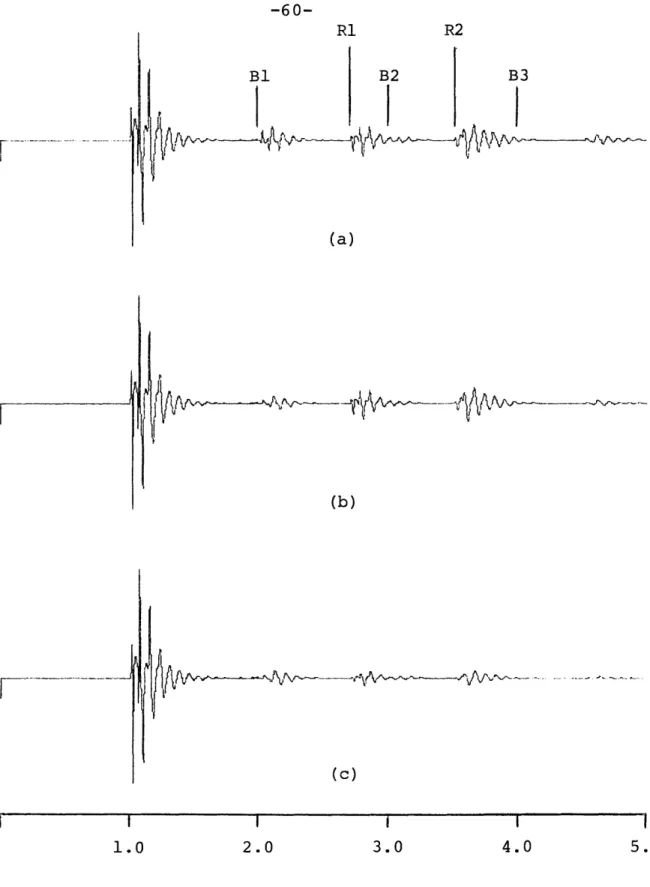
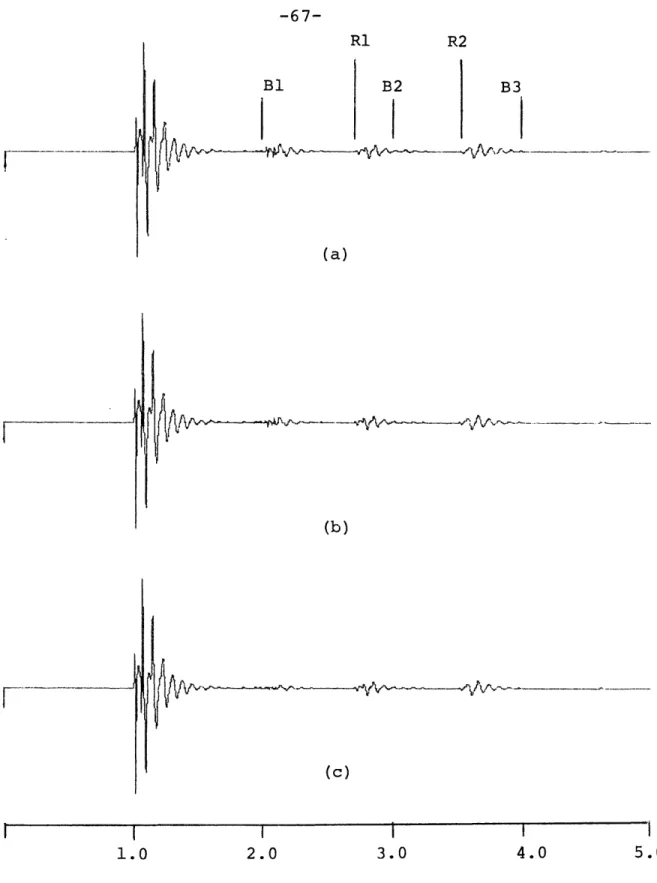
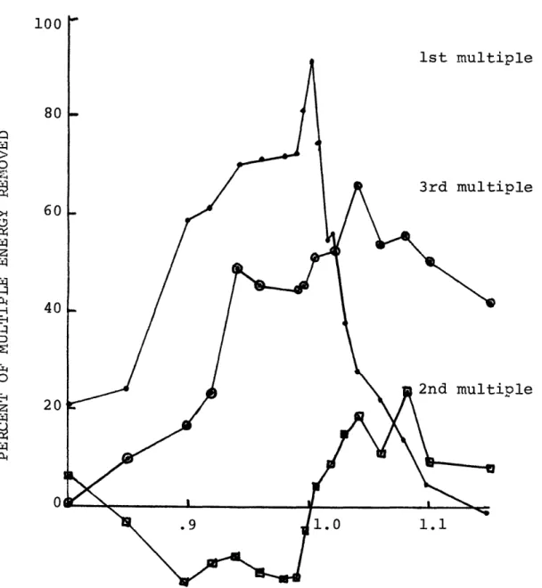
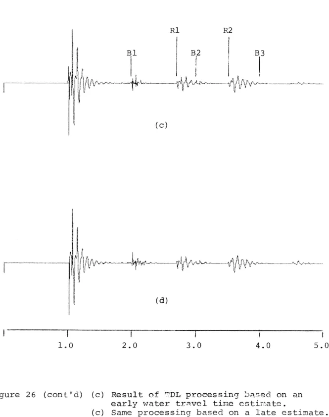
Figure 25 shows the results of water travel time estimation errors for the ideal case of a signal with impulsive multiples. The unprocessed seismogram, shown in figure 26a, contains

reflectors at 2.7 and 3.5 seconds and a strong multiple at 2.0 seconds. The actual two-way travel time in this case is 1.0 second. The strong similarity between the bottom reflection and multiple is apparent.

First multiple energy removed is very sensitive to travel time estimation, with an error of + 10 msec resulting in a performance degradation of about 20%. This effect is analogous to that observed in matched filter receivers in that the

coherent signal components exhibit very high correlation for a small range of lags. In this case the strong coherence and