A comparison of multivariable design methodologies for a two-degree-of-freedom gyro torque-rebalance loop

A Comparison of

Multivariable Design Methodologies

for a

Two-Degree-of-Freedom Gyro

Torque-Rebalance Loop

by

John Ransom Coffee

S.B. Massachusetts Institute of Technology (1986)

SUBMITTED TO THE DEPARTMENT OF AERONAUTICS AND ASTRONAUTICS IN PARTIAL FULFILLMENT OF THE

REQUIREMENTS FOR THE DEGREE OF MASTER OF SCIENCE

at the

MASSACHUSETTS INSTITUTE OF TECHNOLOGY

May, 1988

®

The author hereby grants to M.I.T. and The Charles Stark Draper Laboratory, Inc. permission to reproduce and to distribute copies of this thesis document in whole or in part.

Signature of Author

/Departmei of Aeronautics and Astronautics

.988

Certified by

Professor Wallace E. Vander Velde

Certified by.

Dr. George T. Schmidt

Accepted by

fofe'ssor Harold Y. Wachman

Chairman, Departmental Graduate Committee

MAY 2 4 1988

W

! I DRA WN

A Comparison of

Multivariable Design Methodologies

for a Two-Degree-of-Freedom Gyro

Torque-Rebalance Loop

by

John Ransom Coffee

Submitted to the Department of Aeronautics and Astronautics in partial fulfillment of the

requirements for the degree of Master of Science

ABSTRACT

Multivariable design methodologies are compared in the context of controller design for the torque-rebalance loop for a strapdown two-degree-of-freedom dynamically tuned gyro described by complex coefficient differential equations. The methodologies considered are linear quadratic Gaussian with loop transfer recovery (LQG/LTR), formal loop shaping with LQG/LTR (FLS/LQG/LTR), frequency weighted LQG (FW/LQG), and classical lead compensation. The classical and multivariable methodologies are used to generate low bandwidth controller designs. The multivariable methodologies are also used to generate high bandwidth designs. The performance of the controllers are compared as

well as the design methodologies themselves. The overall performance of the

multivariable designs is much greater than that of the classical design, but com-pensators of approximately double the order are required. There is little

per-formance difference between the multivariable designs. Of those examined, only

the FW/LQG design methodology directly produces compensators that meet all of the typical torque-rebalance loop design requirements. LQG/LTR provides a simple design approach, with the design problem reduced to the selection of two scalar parameters. FLS/LQG/LTR has some promise in torque-rebalance loop design, but more expertise is needed in the selection of suitable target loops.

Thesis Supervisor: Wallace E. Vander Velde

Title: Professor of Aeronautics and Astronautics

Technical Supervisor: George T. Schmidt, Sc.D.

Title: Chief, Advanced Guidance Section,

Advanced Systems Development Division, Air Force and Defensive Systems Department,

Acknowledgement

Completion of this thesis marks the end of my career at M.I.T. I am grateful to my parents for making it possible for me to attend M.I.T. as an undergraduate.

I am especially indebted to my technical supervisor, Dr. George Schmidt of the Charles Stark Draper Laboratory, for sponsoring me as a Draper Fellow. His generous support, understanding and advice made this work possible.

I express deep gratitude to my thesis advisor, Professor Wallace VanderVelde,

for taking on this thesis and providing it with direction and goals. His encour-agement, assistance and concern extended far beyond the scope of this thesis and were greatly appreciated.

I also want to thank Professor Winston Markey for introducing me to control

system design. Special thanks go to Professor Michael Athans for teaching me

multivariable control and for taking the time to explain to me some of the subtleties of the LQG/LTR and FLS/LQG/LTR design methodologies.

I want to thank Tom Thorvaldsen and Mike Luniewicz for taking the time

to answer my questions about the model of the gyroscope and design issues.

I extend sincere thanks to Dr. Frank Saggio and others at Smiths Indus-tries, SLI Division, for sparking my interest in this design problem and for their interest in this work.

This work was performed at The Charles Stark Draper Laboratory under contract F04704-86-C-0160. Publication of this document does not constitute

approval by The Charles Stark Draper Laboratory, Inc. or by the Air Force of

the findings or conclusions contained herein. It is published for the exchange and stimulation of ideas.

I hereby assign my copyright of this thesis to The Charles Stark Draper Laboratory, Inc., Cambridge, Massachusetts.

John R. Coffee

Permission is hereby granted by The Charles Stark Draper Laboratory, Inc. to the Massachusetts Institute of Technology to reproduce any or all of this thesis.

Table of Contents

Abstract

Acknowledgement

Table of Contents

List of Figures

List of Tables

1.21 Strapdown Gyro Operation . . . .... 14

1.2.2 Strapdown Torque-Rebalance Loop Operation ... 15

1.2.3 The Complex Method ... . 17

1.3 Torque-Rebalance Loop Performance Requirements ... 17

1.4 Thesis Goals and Design Approach ... 19

2 Gyro Model Description

20

2.1.1 Background ... 20

2.1.2 The Tuning Condition ... . 21

2.1.3 Gyro Rotor Equations of Motion ... 24

2.2 Torquer and Pickoff Models .. 27

2.3 Linearized Equations of Motion . ... 28

2.4 Application of the Complex Method to the Gyro Model ... 29

2.5 Summary ... 30

3 Properties of Block Symmetric Matrices and Systems

3.2 Definition of Block Symmetric Systems and Complex Notation

3.3 Properties of Block Symmetric Matrices ...

3.3.1 Algebraic Properties . . . .

3.3.2 Eigenvalues and Eigenvectors ...

3.4 Properties of TITOBS Systems ...

31 31 32 34 34 36 38 2 3 4 7 11

3.4.1 Transfer Function Description ...

3.4.2 Transmission Zeros . . . .

3.4.3 Bode Plots ...

3.4.4 Complex SISO Nyquist Criterion ...

3.4.5 Linear Quadratic Regulators ...

3.5 Implementation of Block Symmetric Compensators 3.6 Summary ...

4 Open Loop Gyro Characteristics

4.1 Numerical Values ... 4.2 Complex Modes ... 4.3 Design Plant Model ...

4.3.1 Integrator ... 4.3.2 Demodulation Filter .

4.3.3 Spin Frequency Notch Filter

4.4 Summary ...

5 Design Methodologies

5.1 Background ...

5.2 Overview of Methodologies and Design Approach 5.3 Lead Compensation Design ...

5.3.1 Description of Design Methodology .... 5.3.2 Low Bandwidth Design ...

5.3.3 Performance Limitations of First Order sator Designs ...

5.3.4 Summary ...

5.4 LQG/LTR Design . . . .

5.4.1 Description of Design Methodology .... 5.4.2 Design Approach ...

5.4.3 Linear Quadratic Target Loop Design . .

5.4.4 Recovery of the LQ Target Loops ...

5.4.5 Summary ... 5.5 FW/LQG Design ...

5.5.1 Description of Design Methodology ....

5.5.2 Design Approach ...

5.5.3 FW/LQ Loops . . . ..

5.5.4 Compensator Designs.

5.5.5 Summary ... 5.6 FLS/LQG/ TR Design.

5.6.1 Description of Design Methodology .... 5.6.2 Design Approach ...

5.6.3 Linear Quadratic Target Loop ...

5.6.4 Recovery of the LQ Target Loop ...

. .. Lead . . . .. . .. . .. . .. . .. . .. . ..

...

.139

5.6.5 Target Loops Based on Real Coefficient Gyro Dynamics . 144 . . . . . . . . . . . . . . . . . . . . . . . . . . . .

...

...

5.6.6 Decoupling Compensators.

5.6.7 Summary ... 5.7 Summary ...

6 Comparison of Design Methodologies and

6.1.1 Overview ...

6.1.2 Low Bandwidth Designs ... 6.1.3 High Bandwidth Designs ...

6.1.4 Summary ... 6.2 Design Procedures ...

6.2.1 Classical Lead Compensation . . . 6.2.2 LQG/LTR ...

6.2.3 FW/LQG ...

6.2.4 FLS/LQG/LTR ...

6.3 Conclusions and Recommendations ....

....

149

....

159

....

162

Conclusions

C Correlated Noise Kalman Filter Problem

C.1 Correlated Noise Kalman Filter Derivation ... C.2 The CN/KF Model Based Compensator ...

C.3 Summary of Duality. 163 163 163 165 167 169 169 169 170 171 171 172 173 175 177 182 183 . 183 . 185 . 187 . . . . . .. . . .

List of Figures

1 Introduction

1.1 Momentum Wheel Spinning in Inertial Space 1.2 TDF-DTG Rotor and Suspension Schematic 1.3 TDF-DTG Cross-Section ...

1.4 Torque-Rebalance Loop Block Diagram . . .

2 Gyro Model Description

2.1 Suspension System Schematic Diagram ... 2.2 Suspension System with the Shaft Deflected ...

2.3 Orientation of C-frame and N-frame ...

3 Properties of Block Symmetric Matrices and Systems

3.2 Example Feedback Loop ... 3.3 CCTF Bode Plot of G₀(s) ...

3.4 CCTF Bode Plot of -jG(s) ... 3.5 Complex Unity Gain Feedback Loop ... 3.6 Nyquist Contour ...

3.7 Complex SISO Nyquist Plot of a TITOBS System ... 4 Open Loop Gyro Characteristics

4.1 Bode Plot of the Gyro CCTF, Gp(8) ...

4.2 Real TITOBS System Quadrature Mode Time Response 4.3 Complex System Quadrature Mode Time Response . 4.4 Real TITOBS System Nutation Mode Time Response 4.5 Complex System Nutation Mode Time Response .... 4.6 Torque-Rebalance Loop with Augmented Plant ...

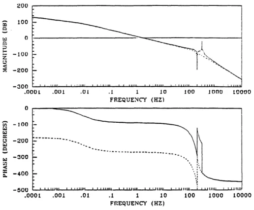
4.7 Design Plant Model Bode Plot ...

4.8 Torque-Rebalance Loop with Augmented Compensator 5 esign Methodologies

5.1 Design Feedback Loop ...

5.2 Design Plant Model Augmented with Notch Filter Bode Plot 5.3 Augmented Lead Compensator Bode Plot ...

5.4 Lead Compensated System Open Loop Bode Plot ...

13 14 15 16 16 20 21 22 25 31 43 44 45 45 46 47 48 53

...

55

... ..

56.

... ..

59

... ..

60

Lead Compensated System Closed Loop Bode Plot.

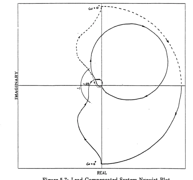
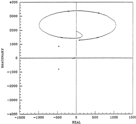
Lead Compensated System Step Response ... Lead Compensated System Nyquist Plot ...

Nyquist Nutation Circle for Increasing Crossover Frequency

LQG/LTR Feedback Loop Block Diagram ...

LQ Feedback Loop Block Diagram ...

Block Diagram of KMBC(S) Modified With Notch Filter . . Low Bandwidth LQ Target Open Loop Bode Plot ...

Low Bandwidth LQ Target Closed Loop Bode Plot ...

High Bandwidth LQ Target Open Loop Bode Plot ...

High Bandwidth LQ Target Closed Loop Bode Plot .... Zero Locus During Recovery of the Low Bandwidth Target

Zero Locus During Recovery of the High Bandwidth Target

Design LQG/LTR-la Augmented Compensator Bode Plot Design LQG/LTR-la Open Loop Bode Plot ...

Design LQG/LTR-la Closed Loop Bode Plot ... Design LQG/LTR-la Step Response ...

Design LQG/LTR-la Nyquist Plot ...

Design LQG/LTR-lb Augmented Compensator Bode Plot . Design LQG/LTR-lb Open Loop Bode Plot ...

Design LQG/LTR-lb Closed Loop Bode Plot ...

Design LQG/LTR-lb Step Response ... Design LQG/LTR-lb Nyquist Plot ...

Design LQG/LTR-2a Augmented Compensator Bode Plot . Design LQG/LTR-2a Open Loop Bode Plot ...

Design LQG/LTR-2a Closed Loop Bode Plot ...

Design LQG/LTR-2a Step Response ... Design LQG/LTR-2a Nyquist Plot ...

Design LQG/LTR-2b Augmented Compensator Bode Plot . Design LQG/LTR-2b Open Loop Bode Plot ...

Design LQG/LTR-2b Closed Loop Bode Plot ...

Design LQG/LTR-2b Step Response ... Design LQG/LTR-2b Nyquist Plot ...

Frequency Weighted LQ Loop Block Diagram ...

Complete FW/LQG Feedback Loop Block Diagram .... Control Weighting Function Bode Plot ...

Closed Loop LQ Bode Plot: Constant State Weighting . . . Step Response: Constant State Weighting ...

Resonant State Weighting Bode Plot ...

Closed Loop LQ Bode Plot: Resonant State Weighting . . . Step Response: Resonant State Weighting ...

Low Bandwidth State Weighting Function Bode Plot ....

Low Bandwidth LQ Design Open Loop Bode Plot ... 5.5 5.6 5.7 5.8 5.9 5.10 5.11 5.12 5.13 5.14 5.15 5.16 5.17 5.18 5.19 5.20 5.21 5.22 5.23 5.24 5.25 5.26 5.27 5.28 5.29 5.30 5.31 5.32 5.33 5.34 5.35 5.36 5.37 5.38 5.39 5.40 5.41 5.42 5.43 5.44 5.45 5.46 5.47

... 69

...

71

...

74

...

82

...

83

...

85

...

90

... 93

...

97

Low Bandwidth LQ Design Closed Loop Bode Plot ... 117

High Bandwidth State Weighting Function Bode Plot ... 118

High Bandwidth LQ Design Open Loop Bode Plot ... 119

High Bandwidth LQ Design Closed Loop Bode Plot ... 120

Design FW/LQG-1 Augmented Compensator Bode Plot ... 121

Design FW/LQG-1 Open Loop Bode Plot ... 122

Design FW/LQG-1 Closed Loop Bode Plot ... 122

Design FW/LQG-1 Step Response ... 123

Design FW/LQG-1 Nyquist Plot ... 124

Design FW/LQG-2 Augmented Compensator Bode Plot ... 125

Design FW/LQG-2 Open Loop Bode Plot ... 126

Design FW/LQG-2 Closed Loop Bode Plot ... 127

Design FW/LQG-2 Step Response ... 128

Design FW/LQG-2 Nyquist Plot ... 129

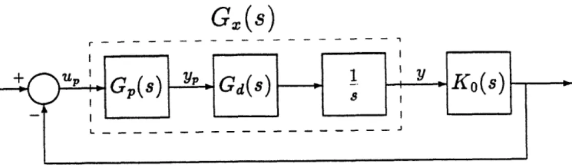
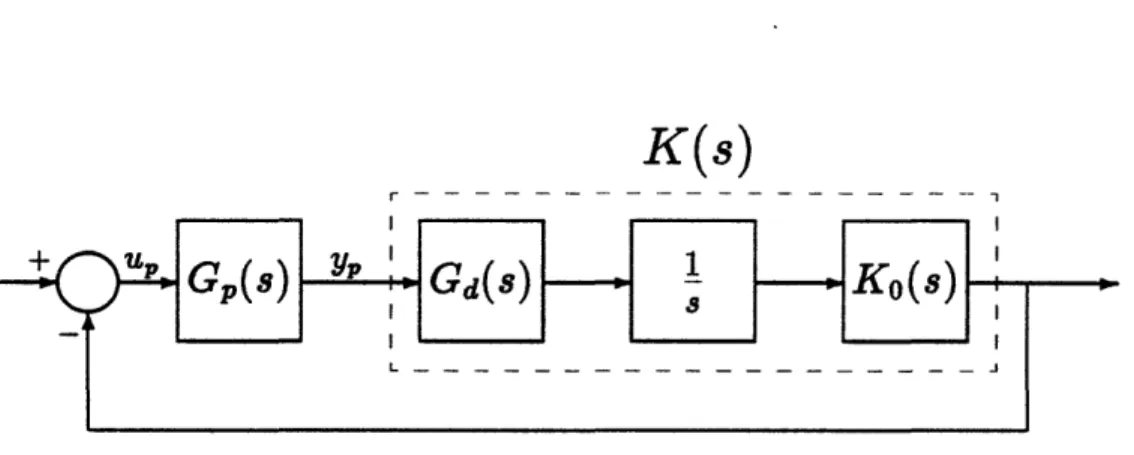
Incorporation of the Target Loop Shape at the Plant Input . . . 132

FLS/LQG/LTR Feedback Loop Block Diagram ... 133

FLS/LQG/LTR Stochastic Model ... 134

Poles of G,(s) and W(s) for Design FLS-0 ... 138

Design FLS-0 LQ Target Open Loop Bode Plot ... 140

Design FLS-0 LQ Target Closed Loop Bode Plot ... 140

Design FLS-0 Augmented Compensator Bode Plot ... 141

Design FLS-0 Open Loop Bode Plot ... 142

Design FLS-0 Closed Loop Bode Plot . . ... 142

Design FLS-0 Step Response to t = 0.1 sec ... 145

Design FLS-0 Step Response to t = 40ec . . . 145

Design FLS-0 Nyquist Plot ... .. 146

Poles of G,(s) and W(s) for Designs FLS-1 and FLS-2 ... 147

Low Bandwidth Target Open Loop Bode Plot ... . 148

Low Bandwidth Target Closed Loop Bode Plot ... 148

High Bandwidth Target Open Loop Bode Plot ... 150

High Bandwidth Target Closed Loop Bode Plot ... 150

Design FLS-1 Augmented Compensator Bode Plot ... 151

Design FLS-1 Open Loop Bode Plot . . . ... 152

Design FLS-1 Closed Loop Bode Plot ... 152

Design FLS-1 Step Response ... . 154

Design FLS-1 Nyquist Plot ... .. 155

Design FLS-2 Augmented Compensator Bode Plot ... 156

Design FLS-2 Open Loop Bode Plot ... 157

Design FLS-2 Closed Loop Bode Plot ... 157

Design FLS-2 Step Response ... . 159

Design FLS-2 Nyquist Plot ... 160 5.48 5.49 5.50 5.51 5.52 5.53 5.54 5.55 5.56 5.57 5.58 5.59 5.60 5.61 5.62 5.63 5.64 5.65 5.66 5.67 5.68 5.69 5.70 5.71 5.72 5.73 5.74 5.75 5.76 5.77 5.78 5.79 5.80 5.81 5.82 5.83 5.84 5.85 5.86 5.87 5.88

C Correlated Noise Kalman Filter Problem

183

List of Tables

4 Open Loop Gyro Characteristics

4.1 Gyro Model Numerical Values ...

5 Design Methodologies

5.1 Lead Compensator Poles and Zeros ...

5.2 Lead Compensated System Closed Loop Poles ...

5.3 First Order Lead Compensation Design Parameters ....

5.4 Low Bandwidth LQ Target Closed Loop Poles and Zeros . 5.5 High Bandwidth LQ Target Closed Loop Poles and Zeros

5.6 Design LQG/LTR-la Compensator Poles and Zeros . . .

5.7 Design LQG/LTR-la Closed Loop Poles ...

5.8 Design LQG/LTR-lb Compensator Poles and Zeros . . .

5.9 Design LQG/LTR-lb Closed Loop Poles ...

5.10 Design LQG/LTR-2a Compensator Poles and Zeros . . .

5.11 Design LQG/LTR-2a Closed Loop Poles ...

5.12 Design LQG/LTR-2b Compensator Poles and Zeros . . .

5.13 Design LQG/LTR-2b Closed Loop Poles ...

5.14 LQG/LTR Compensator Design Parameters ...

5.15 Low Bandwidth Design LQ Closed Loop Poles and Zeros. 5.16 High Bandwidth Design LQ Closed Loop Poles and Zeros 5.17 5.18 5.19 5.20 5.21 5.22 5.23 5.24 5.25 5.26 5.27 5.28 5.29 5.30 5.31

Design FW/LQG-1 Compensator Poles and Zeros...

Design FW/LQG-1 Closed Loop Poles ...

Design FW/LQG-2 Compensator Poles and Zeros...

Design FW/LQG-2 Closed Loop Poles ...

FW/LQG Compensator Design Parameters ...

Design FLS-0 LQ Target Closed Loop Poles and Zeros Design FLS-0 Compensator Poles and Zeros ... Design FLS-0 Closed Loop Poles ...

Low Bandwidth Target Closed Loop Poles and Zeros High Bandwidth Target Closed Loop Polec -:nd Zeros Design FLS-1 Compensator Poles and Zeros ... Design FLS-1 Closed Loop Poles ...

Design FLS-2 Compensator Poles and Zeros ... Design FLS-2 Closed Loop Poles ...

FLS/LQG/LTR Compensator Design Parameters . . .

63 67

....

70

....

89

....

97

....

121

... . 123

....

127

....

161

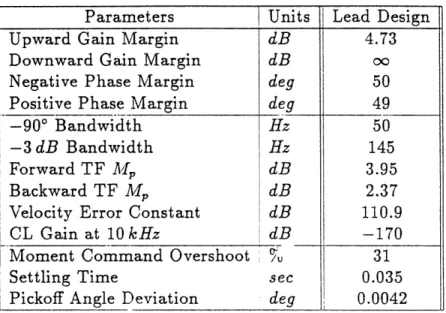
6 Comparison of Design Methodologies and Conclusions 163 6.1 Low (50Hz) Bandwidth Compensator Design Parameters .... 164 6.2 High (100 Hz) Bandwidth Compensator Design Parameters . . . 165

C Correlated Noise Kalman Filter Problem

183

Chapter 1

Introduction

1.1 Overview

This thesis presents a comparison of some multivariable design methodolo-gies. The comparison is based on the specific example of a strapdown, two-degree-of-freedom dynamically tuned gyro torque-rebalance loop. The gyro model is expressed in terms of complex coefficient differential equations, and the controllers are designed for this complex plant description. The performance

of several torque-rebalance loops designed using modern, multivariable design

methodologies and by classical techniques is compared.

The thesis is organized as follows. The remainder of this chapter provides background on the two-degree-of-freedom dynamically tuned gyro, the opera-tion of the torque-rebalance loop, and the complex method. It also describes the thesis goals and overall approach to the design problem. The gyro equa-tions of motion are derived in Chapter 2. The complex method is applied to the linearized equations of motion to yield the complex coefficient differential

equations on which the controller designs are based. Several properties of

sys-tems described by complex coefficient differential equations are summarized in Chapter 3. The design tools presented are used in the subsequent chapters in the design and analysis of the torque-rebalance loop controllers. The open loop characteristics of the linear gyro model are analyzed in Chapter 4. The

controller designs are presented in Chapter 5. Each design methodology is

de-scribed, and the design approach used for each methodology is presented. The unique characteristics and performance of the resulting loop designs are also discussed. Finally, a comparison of the design methodologies and conclusions are included in Chapter 6.

1.2 Background

1.2.1

Strapdown Gyro Operation

Over the past twenty years, the two-degree-of-freedom dynamically tuned

gyro (TDF-DTG) has gained widespread use in strapdown inertial

naviga-tion systems as an angular rate sensor. The TDF-DTG, like single-degree-of-freedom floated instruments, uses a momentum wheel to measure angular rates.

t

M w

Figure 1.1: Momentum Wheel Spinning in Inertial Space

A schematic of a rotor spinning in inertial space is shown in Figure 1.1. The rotor spins with constant angular momentum, H. The motion of the rotor is governed by the equation

dt-M= dH+ ,xK

(1.1)

where M is a torque applied to the rotor and wa is the precession of the rotor with respect to inertial space in rotor coordinates. The angular momentum in

(1.1) is assumed to be constant so the derivative term is zero. If no torques are

applied to the rotor, it will maintain its orientation in inertial space, conserving angular mom-entum. If a torque perpendicular to the spin axis is applied to the rotor, the rotor will precess at the rate w about an axis perpendicular to the spin axis and the axis of the applied torque.

Figure 1.2 shows a schematic diagram of a TDF-DTG. The rotor is attached

Flexures X I lr--~ tlbal Rotor

In

Figure 1.2: TDF-DTG Rotor and Suspension Schematic

The shaft is driven at a constant speed, wo, by a motor which is attached to the

gyro case (not shown). The flexures are stiff in bending but compliant in torsion, allowing the rotor, through the gimbal, to precess about the x and y-axes shown in the figure. This provides the instrument with the capability of sensing inertial

angular rates on two axes simultaneously.

The torsional spring constants of the flexures, gimbal inertias, and rotor spin speed are chosen together such that the torque on the rotor due to the flexure spring rates cancels the torque due to the dynamically induced spring rate. The result is that the net average torque on the rotor due to the suspension system

is zero, and the rotor behaves like a free body. This is known as the tuning

condition and is described in Chapter 2.

A cross-section of a TDF-DTG is shown in Figure 1.3. The rotor is driven by the motor at the base of the gyro case. The angle between the rotor and the case is measured electromagnetically by two sets of variable inductance type

pickoffs, one pair on each axis. A pair of torquer coils, fixed to the case, on each

axis apply torques to the rotor electromagnetically as well. Current through the coils acts with the magnets fixed to the rotor to precess the rotor about the desired axis.

1.2.2 Strapdown Torque-Rebalance Loop Operation

A momentum wheel gyro employed in the strapdown mode makes use of the gyroscopic properties discussed above. A block diagram of a torque-rebalance loop is shown in Figure 1.4. In a strapdown application, the gyro case is bolted

to the vehicle and is subjected to the inertial angular rates experienced by the C- WS

Stop

Suspension

Rotor

Figure 1.3: TDF-DTG Cross-Section

b Inertial Angular Rate

ie

nand

vehicle. No torques are applied to the gyro rotor about its input axes by the suspension system so the rotor remains at a constant attitude with respect to inertial space. The resulting angular offset between the case and rotor, , is

measured by the pickoffs and is called the pickoff angle. This signal is fed to the

controller which generates a commanded torque, M, to be applied to the rotor in such away as to precess the rotor at a rate equal to the inertial angular rate applied to the gyro case, thus driving the pickoff angle back to null.

This commanded torque is also the output of the torque-rebalance loop used by the attitude update algorithm of the inertial navigation system as a measure of the inertial angular rate. This relationship can be seen in Equation (1.1) since the precession rate is equal to the inertial angular rate, and the angular momentum of the rotor is known. Thus, the torque-rebalance loop is used to keep the rotor spin axis perpendicular to the gyro input axes, keeping the pickoff angles nulled, and its output, the commanded torque, is used as a measurement of the inertial angular rates to which the gyro case is subjected.

1.2.3 The Complex Method

The complex method has been used to simplify the analysis of rotationally symmetric systems for quite some time. It was first applied to the analysis of

a two-degree-of-freedom gyro two decades ago [13]. The primary advantage of

the complex method is that it turns the two input-two output real gyro model

into a single input-single output (SISO) system described by complex coefficient differential equations. This in turn allows classical SISO design tools to be used

in the analysis of a nominally multi-input-multi-output (MIMO) system. The complex method is discussed in Chapter 3.

1.3 Torque-Rebalance Loop Performance

Re-quirements

The torque-rebalance loop design requirements are typical of all regulator loops: good distlrbance rejection, noise attenuation, and high bandwidth while maintaining sufficient stability margins. The requirements for the loop are driven by the specific dynamics of the gyro and the need for accurate inertial angular rate measurements for the inertial navigation system. The performance of the

inertial navigation system attitude algorithm depends directly on the frequency and time domain characteristics of the torque-rebalance loop. The torque com-mand fed to the gyro must accurately reflect the angular rate environment of the vehicle so that the attitude algorithm has an accurate measurement of the inertial angular rates and so that accurate operation of the gyro can be ensured. In order for the torque-rebalance loop to provide accurate measurements of inertial angular rates, the rotor spin axis must always be perpendicular to the

gyro input axes, that is, the pickoff angles must always be nulled. Therefore,

the controller must provide torque commands that will precess the gyro at the angular rates expected to be encountered by the vehicle with minimum error. In this context, the inertial angular rate applied to the gyro case can be thought of as a disturbance input that must be rejected by the regulator. This requires a high bandwidth loop with large velocity or acceleration error constants.

It is desirable for the torque command to be as free of noise as possible.

Two major noise sources are vibration at the shaft spin frequency and high frequency noise due to pickoff signal modulation. Therefore, loop gain at the

spin frequency must be as low as possible, effectively limiting the bandwidth of

the loop to below the spin frequency. In addition, the high frequency roll off of the torque-rebalance loop gain must be as great as possible to attenuate noise at the pickoff signal modulation frequency.

The computational bandwidth of the attitude algorithm is taken to be half of the attitude update rate. The bandwidth of the torque-rebalance loop should be equal to the computational bandwidth so that the attitude algorithm will have angular rate information over its entire bandwidth. In addition, the loop gain within the bandwidth must be as near unity as possible. If the vehicle is subjected to coning motion within the torque-rebalance loop bandwidth and the closed loop gain at the coning frequency is not unity, the attitude algorithm will produce rectified attitude errors proportional to the square of the closed loop gain [4], which cannot be compensated with coning compensation algorithms.

The torque-rebalance loop design must also have sufficient stability margins so that the loop will remain stable in the presence of modelling errors, pickoff and torquer misalignments, and changes in operating conditions. The above

1.4 Thesis Goals and Design Approach

Historically, classical design techniques have been used for the design of torque-rebalance loop controllers [15], [3], and [11]. Only recently have

mod-ern, multivariable design techniques been examined for use in this problem [16]. The goal of this thesis is to compare some multivariable design methodologies in the context of the torque-rebalance loop example. The methodologies consid-ered are linear quadratic Gaussian with loop transfer recovery (LQG/LTR),

for-mal loop shaping with LQG/LTR (FLS/LQG/LTR), frequency weighted LQG

(FW/LQG), in addition to classical lead compensation. The design methodolo-gies are described in Chapter 5.

As stated above, several torque-rebalance loop controllers are designed for a continuous time gyro model described by complex coefficient differential

equa-tions. A first order lead design, which has been typically used in classical loop

designs, provides a low bandwidth baseline design. The multivariable

method-ologies are used to generate low bandwidth designs that are compared to the classical lead design. These methodologies can be used to generate much higher

bandwidth designs; therefore, high bandwidth multivariable designs are also

compared.

The performance of the controllers are compared as well as the design method-ologies themselves. The results of these comparisons are summarized in Chap-ter 6. The overall performance of the multivariable designs is much greaChap-ter than that of the classical first order lead, but they require compensators of approx-imately double the order of the classical design. There is little performance

difference between the multivariable designs however. Of those examined, only

the frequency weighted linear quadratic Gaussian design methodology produces compensators that meet all of the typical TDF-DTG torque-rebalance loop sign requirements directly through the design methodology. The LQG/LTR de-sign methodology provides the easiest dede-sign approach, with the dede-sign problem reduced to the selection of two scalar parameters. Finally, the FLS/LQG/LTR

design approach has some promise in torque-rebalance loop design, but more expertise is needed in the selection of suitable target loops.

Chapter 2

Gyro Model Description

In this chapter, the linear model of the gyro used in the design of the

torque-rebalance loop controllers is discussed. First, the dynamics of a single gimbal

rotor suspension system are analyzed in order to derive the tuning condition. Then the equations of motion of the gyro rotor are derived and linearized to generate the linear model used in the design analysis. Finally, the complex method is applied to the linearized equations in order to take advantage of the rotationally symmetric properties of the gyro.

2.1 Gyro Equations of Motion

2.1.1

Background

The dynamics of practical two degree of freedom, tuned gyroscopes have been well understood for nearly two decades. Accordingly, there are several

deriva-tions of the equaderiva-tions of motion available. Savet [14] derived the equaderiva-tions of motion for a gimballess, "vibra-beam" gyro using a Lagrangian potential. An alternative derivation is presented by Craig [6], who derived the equations of motion for a dynamically tuned gyro with n gimbals using a Newton-Euler approach. Craig [5] also performed extensive analysis on the error sources as-sociated with a physical gyro. In a subsequent paper, Craig [4] derived the equations of motion for a physical tuned gyro under the assumption that the gyro rotor is a free body and then introduced terms corresponding to the error sources of a physical gyro into the free body equations of motion. A detailed

analysis of a one and two gimbal gyros is also presented in [3].

The derivation of the equations of motion for a single gimbal, tuned gyro that is presented in this thesis follows the approach taken by Craig [4]. This analysis

z, zW

zg

C)WS

Xi

yI Y;ry9

wS Z? t

Figure 2.1: Suspension System Schematic Diagram

has been simplified somewhat to include the effects of an imperfect suspension

system only, which have a first order effect on the gyro rotor motion, ignoring

pickoff and torquer misalignments and other effects. A description of the overall

gyro system is presented in Section 1.2.1.

2.1.2

The Tuning Condition

A schematic diagram of the gyro shaft, rotor, and suspension system is shown in Figure 2.1. Four reference frames are used in the analysis of the suspension system. The i-frame is fixed in inertial space; the r-frame is fixed in the gyro

rotor; the g-frame is fixed in the gimbal, and the s-frame is fixed in the gyro

shaft. The shaft y-axis, y, coincides with the gimbal y-axis, and the gimbal x-axis, xg, coincides with the rotor x-axis, x. The rotor has an angular velocity of w, with respect to inertial space about its z-axis, which is'aiigned with the

inertial z-axis, zi.

A diagram showing the shaft deflected with respect to the rotor is shown in Figure 2.2. The instantaneous attitude of the shaft relative to the rotor is

.9

z

%z

z

Fr

5:

XY

Figure 2.2: Suspension System with the Shaft Deflected

defined by the two angles, Wm and cpy, which are assumed to be small.

The moment applied to the rotor about the x'-axis is the combined torsional spring constant of the outer flexures, Kc, multiplied by the deflection angle, yp.

An = Kmcp, (2.1)

The moment applied to the rotor about the y'-axis is the difference between the moment applied to the gimbal about the y-axis by the inner flexures, K,y,, and the inertia moments of the gimbal about that axis.

M; = Ky

- [Iigy - (Igz - Ig,) wgzw9]

(2.2)

x9, yg, and z, are denoted by Ig_, Igy, and Ig, respectively.

The angular velocity of he gimbal with respect to inertial space, written in

gimbal coordinates is

W=

Y

(2.3)

tgy - W.

]

g

Its value is found from:

= Wg + C

;ig ~ 7-rg -sr

with

g = [0 W, = 0

and where C9 is the direction cosine matrix relating the r-frame to the g-frame.

Assuming W, and py are small, it is shown below.

1 0 0

C, = 0 1

0 - 1

Substituting Equation (2.3) into Equation (2.2) yields the two equations for the moments applied to the rotor by the suspension system in rotor coordinates.

M;rr = K. P (2.4)

M = K y + (-Igz -Igy + Ig,,)

w..

WP = 0. cos W't (2.6)

WY = -O, sinwot. (2.7)

Substituting Equations (2.6) and (2.7) into (2.4) and (2.5) yields the following moment equations

Mr. = K2.O.cosWt (2.8)

Mr

-[Ky +

+Ig )

,t.

After some manipulation, Equations (2.8) and (2.9) can be written in inertial

coordinates as shown in Equations (2.10) and (2.11).

=

[(K. + K) + (-Ig-Ig+I

gz)w:]

+

{ [(K - K) -(-Igz,. - Igy + Igz) ,,] .2 COS 2wt (2.10)

An ideal suspension system would transmit zero average moment to the rotor

regardless of the time history of qO. For the case of a constant b, the average

moment equations are

1

[(K + Ky)+(-I,.

-I,,

+ I) w

_(2.12)

MrY = O. (2.13)

Equation (2.12) suggests the tuning condition. If the flexure torsional spring constants, gimbal moments of inertia, and rotor spin angular velocity can be chosen according to (2.14), the suspension system is said to be tuned.

= IK + Ky . (2.14)

As a result, the rotor is decoupled from the suspension system, and the average moments on the rotor due to the suspension system are zero.

2.1.3

Gyro Rotor Equations of Motion

The equations of motion of the gyro rotor are derived under the assumption that the tuning condition is met, so that the gyro rotor behaves like a free rotor in inertial space. Terms corresponding to moments due to an imperfect suspension system are added to the free body equations of motion to complete the model.

It is convenient to derive the equations of motion using coordinate systems that do not rotate with the rotor because the gyro pickoffs and torquers are

fixed to the gyro case. Therefore, two new coordinate frames are defined. The

frame is attached to the rotor but does not spin with the rotor, and the

n-frame z-axis is aligned with the rotor spin axis. The c-n-frame is fixed in the gyro

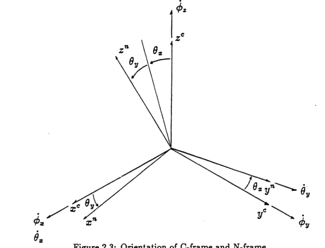
case. Figure 2.3 shows the relationship between the n-frame and the c-frame. The orientation of the n-frame with respect to the c-frame is defined by the two

pickoff angles 0. and Oy.

The angular velocity of the n-frame with respect to inertial space written in the n-frame is

win =

=Cc

+

(2.15)

where

17

I

Figure 2.3: Orientation of C-frame and N-frame

The direction cosine matrix, C,', for small 8, and Ov is shown below.

1 0 -8y

C n = O 1 0

B0 -0. 1

Substituting the above quantities into Equation (2.15) yields Equation (2.16).

Wn[ 1 + 0 - 1yo.

Wi.n W ny= +y + Y +, (2.16)

JWnzq

1kzi

The moment on the rotor, written in the n-frame, is equal the the rate of

change of its angular momentum, as shown in Equation (2.17).

= (H) = () + x H (2.17) The angular momentum of the rotor is

IrWnz

J

n = IryWnyW, (2.18)

Irz (nz + W.)

where w, is the rotor spin speed, which is assumed to be held constant by the gyro

motor and is much larger than wnz,, and I,, Iy,, and I,, are the rotor moments of inertia about the corresponding rotor axes. Substituting (2.16) and (2.18) into (2.17) yields the following moments on the rotor, written in the n-frame.

[Ir

Mn = Iryny + (Ir. -

I,.z)

,wnz,

-

IIzw,

(2.19)

IrzI nz + (Iry -r)Wn=Wny

The moment on the rotor can be expressed in the case fixed coordinate frame

as shown in (2.20).

ME = C Mn (2.20)

The motor shaft lies along the case fixed z-axis, and under the free rotor as-sumption, can only provide moments to the rotor about this axis. Moments applied to the rotor along the perpendicular axes, Mc,, and My, are provided by the gyro torquers.

Up to this point, the moments on the rotor have been derived under the assumption that the rotor is a free body. Actual rotor suspensions are not ideal,

and their imperfections can be easily modelled as additional sources of moments

on the rotor. These moments can be due to the effects of mistuning, suspension damping, and other imperfections. Craig has described several sources of errors in a dynamically tuned gyro in great detail [5].

For the purposes of this analysis, only the linear terms associated with the moments due to suspension damping will be included. These moments are shown

below in Equations (2.21) and (2.22).

M.C, = HO + DJR, (2.21)

MC =

_ 0

+

DRy

(2.22)

offset. The rotor damping term, DR, is zero in an ideal gyro. It corresponds to

viscous damping and tends to damp rotor nutation oscillations.

M.

=

M + yM + .

S/= Mry-.M + MY

Expanding

Ir

= Iy =

these equations and assuming that the rotor is symmetric so that

I,, yields:

+

I,,

-H

+

-9+DRiz

O

= Ir I

-

H(. + i

(Ir.-

Ir)

Rz)

-o+z)

+

-

0

Irz (E + oy+ + iY+ - 2§

H

-r + DRiy

±

o

-

owy)

When the gyro case is subjected to an inertial angular rate,

4,

2.2 Torquer and Pickoff Models

The gyro torque generators apply commanded moments to the rotor electro-magnetically. An electrical coil is fixed to the gyro case, and a current through the coil acts with permanent magnets on the rotor to magnetically torque the rotor. The torque generator is modelled as a simple gain, KT, with units of torque per millivolt.

The pickoff signal generators also work electromagnetically. A coil is fixed to

the gyro case, and the variation of the inductance of the coil due to rotation of the rotor about the xC-axis and yc-axis is measured by the pickoff. The pickoff output is amplified by a pre-amp and is modulated on a high frequency carrier

(2.24).

(2.23)

(2.24)

signal. The combined pickoff, pre-amp, and signal generator is modelled as a simple gain, KPO, with units of millivolts per radian.

2.3 Linearized Equations of Motion

The equations of motion in (2.25) and (2.26) can be simplified by assuming

that products including the pickoff angles, 80 and ,, are small and retaining only the linear terms of the derivatives of . These linearized equations are

shown below.

MZ = I (

+

i.)

+

H ( +

y) +

DR

+ HB

MY = I,. ( + y)-H ( + Ha)

+ DRiy- H m

(2.27)

(2.28)

The linearized model of the gyro can be expressed in the state space in (2.29) and (2.30).

= Ax + B + Lid + L

d2

Y = Cr

The state vector, x, is made up of the pickoff angles and their derivatives; the control input, u, consists of the moments applied to the rotor by the gyro torquers; the output vector, y, consists of the rotor pickoff angles. The additional inputs, d1and d2 are the inertial angular rates and accelerations. The state space

form of (2.27) and (2.28) is shown below.

0 1 0 0

0

_D

_

H

Irv TIr, Irr

0 0 0 1 H H 0 _ DR

-tir Irr

I, .

-1

[sd]

ooo]

Lt

M1 +

[

i

]

I

2.4 Application of the Complex Method to the

Gyro Model

The complex method has been used to simplify the analysis of a large class of systems with rotationally symmetric dynamics. It has been applied to the two-degree-of-freedom-dynamically tuned gyro by Lipman [13], Craig [6], and others. The application of the complex method to two input-two output block

symmetric (TITOBS) systems has been analyzed in great detail by Johnson [12], and many of his results, discussed in Chapter 3, are used in the remainder of this thesis.

The complex method is applied to the gyro equations of motion by defining

the following complex variables:

c = 0 + jy

Xc = 00+i A

MC = M+ jMy.

Expressing Equations (2.29) and (2.30) in terms of the complex pickoff angle,

OC, complex inertial angular rate,

ke,

the set of complex state space equations shown in (2.33) and (2.34).

r

[ [ + )[ Irr ]

O Irr

]

[

]c

[

[ O[ ]

(2.34)

Clearly, there are several advantages to representing the system in complex form. The two primary reasons that this is done are that a TITOBS system is transformed into a SISO system and that the order of the system is reduced by a factor of two. Addi'._onal properties of TITOBS systems and their complex

representations are discussed in Chapter 3.

It is also convenient at this point to introduce the torquer and pickoff gains into the state equations, and to also write the angles in units of degrees instead

command in millivolts and ' is the pickoff angle output, also in millivolts.

[0c] [0 1 8 0 1

[

ic

(

irr+i

I)

]

[ fc

]±[Kr

[ H o- [ c Q] 0 (2.35)

of

Throughout the remainder of this thesis, the terms in Equations (2.35) and

(2.36) are referred to as the corresponding terms in Equations (2.37) and (2.38).

ip = Apgp + Bpup +

+

LpC

(2.37)

yp = CPp (2.38)

The SISO complex coefficient transfer function from the moment command in-put, up, to the pickoff angle outin-put, yp, is determined from the state space representation of the system as shown in Equation (2.39).

Gp(s) = Cp (sI - Ap)- _{Bp (2.39)}

2.5 Summary

In this chapter, the equations of motion for the two-degree-of-freedom, dy-namically tuned gyro are derived. These equations lead to a linear model of

the gyro used in design and analysis of torque-rebalance loop controllers for the

gyro. The complex method is applied to the linear equations of motion, yielding

Chapter 3

Properties of Block Symmetric

Matrices and Systems

In this Chapter, some properties of block symmetric systems are presented, with special attention to real, two input-two output block symmetric (TITOBS) systems. After some background is presented, block symmetric matrices are

defined, and the relationship between block symmetric systems and their

corre-sponding complex representations is discussed. Next, some properties of block

symmetric matrices are presented. Then some properties of TITOBS systems and their corresponding complex single input-single output (SISO) forms are examined. Included in this section is a discussion of the use of Bode plots of complex systems and the complex SISO Nyquist criterion for control system design. Lastly, the implementation of block symmetric dynamic compensators in digital computers by taking advantage of the complex method is analyzed.

3.1 Background

The linear model of the two-degree-of-freedom tuned gyroscope, along with many other systems with rotational symmetry, is a block symmetric system. This block symmetric nature can be taken advantage of by using the complex method, and the complex method has been used to simplify the analysis of several systems with rotational dynamics. As was discussed in Chapter 2, the complex method has been used to derive the equations of motion of the tuned gyr¢ .nd has also been used to arrive at a complex coefficient transfer function

description of the linearized gyro model ([13] and [61). The use of the complex

method also has advantages in control system design, analysis, and implemen-tation for block symmetric systems, especially TITOBS systems.

Since TITOBS systems can be transformed into complex SISO systems via

the complex method, classical SISO design tools can be used in the design of a

nominally MIMO system. Root locus, Bode plots, and the Nyquist criterion can

be used, but must be interpreted differently for complex systems than for real systems. A 1974 NASA report [15] used the complex versions of root locus and

Bode plots in the design of a tuned rotor gyro torque-rebalance loop controller.

Johnson [12] derived the rules for the root locus of complex systems and also

developed interpretations of Bode plots and the Nyquist criterion for complex

systems; both of which are used extensively in this thesis.

The reduction in system order and number of inputs and outputs afforded

by the complex method offers a possibility of computational savings in

com-pensator design. Comcom-pensators for block symmetric systems implemented in digital computers can benefit from reduced memory storage requirements if the

complex version of the compensator is used.

3.2 Definition of Block Symmetric Systems and

Complex Notation

This chapter describes several properties of real, block symmetric matrices and systems. A 2n x 2m real matrix, S, is block symmetric if it can be partitioned

as shown in Equation (3.1).

S =[ -SiS

i

The real sub-matrices, S, and Si, both have dimension n x m. The complex matrix, S,, corresponding to the real block symmetric matrix, S, is defined in

(3.2).

S = S, + jS

(3.2)

A real, linear, time invariant system that is block symmetric can be described

by a corresponding system in complex form. This is shown to be true for the

gyro model at the end of Chapter 2. Consider the real, block symmetric system

shown below in state space form

i(t) = A(t) + Bu(t)

(3.3)

with the control law

(t) = -G(t) (3.5)

where the matrices A, B, C, and G are properly sized, block symmetric, and are partitioned as

A =

A

B =e

-Bi

A, Bi B,

Ci C Gi G,

and the state, control, and output vectors are partitioned as

2= Mr

j

Next, consider the corresponding complex-system shown below

i>(t) = Axc(t) + B__(t)

(3.6)

y0(t) = C4c(t) (3.7)

with the control law

u(t) = -Gc

(t)

(3.8)

where the complex matrices and vectors are defined as

AC = A, + jAi

Be = B,

+

jBi

Cc = Cr+ jCi

Gc = G, + jGi

EC

= gr + izi

ye = y, +jyi.

The real, block symmetric system described by Equations (3.3) through (3.5) is fully described by the real and imaginary parts of the corresponding complex system in Equations (3.6) through (3.8). This result has some important impli-cations. First, the size of the complex state vector is half the size of the real state vector, since its real and imaginary parts contain the information of the

full size, real vector. Also, the size of the control and output vectors are likewise

halved in the complex description of the system. This is particularly useful if the original real system is TITOBS, since the real system is transformed into

a complex SISO system. This allows modified classical SISO design tools such

as root locus, Bode plots and Nyquist plots to be used for the design of what is physically a two input-two output system. Finally, block symmetric compen-sators implemented in digital computers can also benefit from the use of the complex form of the system, since the memory required to store the smaller

complex matrices is less than that required for real block symmetric matrices.

3.3 Properties of Block Symmetric Matrices

3.3.1

Algebraic Properties

Sum

The sum of two compatible, block symmetric matrices is block symmetric. If R and S are real, block symmetric matrices with

R =

-R. ] S = [

Si

then their sum is shown below

T =R+S

r

T = R + Se

R

=

+

jR

Product

The product of two compatible block symmetric matrices is block symmetric. If R and S are real, block symmetric matrices with

R =

. - Ri

S

S

-Si

then their product is shown below

T= RS

1

J

T = RcSc

RC =

R,

+ jRi

S =

S,+jS

.

Matrix Exponential

The matrix exponential of a block symmetric matrix is block symmetric. If

S is a real, square, block symmetric matrix with S - 1S -Si l

[

Si S"]

then the matrix exponential is shown below

1 1S

T = I+ S+

S2

+ S3 + ...

[ Re{T} -m

{T}

1

J

=

+

s +!

3!

Sc = S,+j .S

Matrix Inverse

The inverse of a block symmetric matrix, if it exists, is block symmetric. If

S is a real, square, block symmetric matrix with

s

=[S

-Si

[

e{S-l} -m{S-n

.

Sc = S, +ji.

#

Determinant

The determinant of a real, square, block symmetric matrix, S, with

s

[St

-]Si

Si St

is

det(S) = [det(S, +

[det(S, - jSi)]

(3.9)

= [det(S.)] [det(Sc)]* (3.10)

where

Sc = S + iS

3.3.2

Eigenvalues and Eigenvectors

The eigenvalues of a real, square, block symmetric matrix come in complex conjugate pairs for both real and complex eigenvalues. The eigenvalues of the real, block symmetric matrix, S, with

S=[S,

-Si1

Si S,

are the eigenvalues, A, of the complex matrix

and their complex conjugates, A*. Therefore, the eigenvalues of a block

sym-metric matrix can be found from the eigenvalues of the corresponding complex matrix.

The right eigenvectors of the real, 2n x 2n, block symmetric matrix, 5, can be found from the eigenvalue problem shown in Equation (3.11)

Sy =

Ak~y k

=

1,2,3,...

,2n

(3.11)

where vk is the kth right eigenvector and Ak is the kth eigenvalue, generally complex. Equation (3.11) can be partitioned as shown in (3.12).

[S

-Si

=

Ak

~]

(3.12)

The n x 1 sub-vectors, vu and , are the upper and lower partitions of the 2n x 1

right eigenvectors.

The right eigenvectors of the corresponding complex, n x n matrix, S,, can be found from the eigenvalue problem shown in Equation (3.13)

S.vi = Acv (3.13)

where

SC = S,.+jSi

V = ' + jivi,

and the subscripts have been removed to simplify the notation. The vector,

vc, is an n x 1 right eigenvector and Ac is its associated eigenvalue, generally complex.

The eigenvectors, v, of the real, block symmetric matrix S can be found from the eigenvectors, v_, of the corresponding complex matrix, Sc. The exact relationship between these eigenvectors depends upon whether the associated

eigenvalues are real or complex.

For a real eigenvalue of Sc, s = A,, the eigenvalues of S are s = Ac and s = A* = A. The associated eigenvectors of S are

For a complex eigenvalue of S, = A,, the eigenvalues of S come in the

complex conjugate pair, = A and s = A*. The associated eigenvectors of S are, respectively

_jv and _v (3.15)

Equations (3.14) and (3.15) can be used to find the eigenvectors of a block

symmetric matrix from the eigenvectors of its corresponding complex matrix.

They can also be used to find the eigenvectors of the complex matrix from those

of the block symmetric matrix. A more detailed discussion and proof of (3.14)

and (3.15) is given by Johnson [121.

3.4 Properties of TITOBS Systems

In this section, some properties of TITOBS systems are discussed. The trans-fer function matrix of a TITOBS system is considered. The complex method yields the SISO complex coefficient transfer function (CCTF). This SISO

trans-fer function allows the use of the complex versions of the Bode and Nyquist

tools. Transmission zeros of TITOBS systems are also examined.

3.4.1 Transfer Function Description

The transfer function matrix of a real, linear, time invariant system relates the Laplace transform of the input vector to the Laplace transform of the output

vector. This relation is shown in Equation (3.16).

Y(s) = G(s)U(s)

(3.16)

UL(s)

can be found from the state space representation of the system from

G(s), = C (sI - A)

' B

(3.17)

If the system is a TITOBS system, then (3.16) can be partitioned in the following manner,

[

where all of the partitioned elements are scalars. The complex method is now

used to generate the complex coefficient transfer function (CCTF), Go(s), which is a scalar function and is shown in Equation (3.19).

G,(s) = G,(s) + jGi(s)

(3.19)

The complex version of (3.18) becomes

Yc(s) = G,(s)Uc(s). (3.20)

The complex time domain input to the system can be partitioned into its real and imaginary parts as

u,(t) = u.(t) + jui(t),

U,(8) = U,(s) + jUi().

The Laplace transform of the output is

Y(S) = Y(s) + jYi(s),

and the complex time domain system output, yc(t), can be found from the inverse

Laplace transform of Y0(s):

yc(t) = y,(t) + jyi(t)

y,(t) = Re{ {

_{

_Y(s)}}

yi(t) =

{&

where £-1 denotes inverse Laplace transform.

One important fact about the CCTF is that it is not conjugate symmetric. Ordinary, real coefficient transfer functions have the property that,

G(s*) = G*(8)

however, for the explicitly complex transfer function,

Gc(s*)

= G,(*) + jGi(*)

= G(s) + jG(s)

but,

therefore, for nonzero G(s),

The result of this lack of symmetry is that the frequency response of the complex

system is different for positive and negative frequencies, yielding two different

Bode plots. Also, the Nyquist plot of a complex system is not symmetric about the real axis. Conjugate symmetry does hold if Ge(s) has real coefficients only.

3.4.2

Transmission Zeros

The transmission zeros of a TITOBS system are the zeros of the correspond-ing CCTF and their complex conjugates. The transmission zeros of a MIMO system come from the solution to the generalized eigenvalue problem shown in

Equation (3.21)

(zkM

where

M=

and k is the kth transmission zero and v_ is the associated right generalized

eigenvector.

The transmission zeros are the roots of

det (zkM - L) = 0 (3.22)

det [zI - A] ldet [C (zI- A)-' B] = 0 (3.23)

det [zI - A] det [G(zk) = 0 (3.24)

if there are no pole-zero cancellations, that is det [zkI - A]

#:

condition, the transmission zeros are the solutions to Equation (3.25).

det [G(zk)] = 0 (3.25)

If the system is a TITOBS system, the transfer function can be expanded as in Equation (3.18). Using the determinant rule in Equation (3.9),

det [G(s)] = [det (G,(s) + jGi(s))] [det (G,(s) -jG(s))] = [det (G,(s))] [det (G,(s*))]

since G,(s) is a scalar function. Therefore, the transmission zeros of a TITOBS system come from the solution to

G,(s) = 0 and G,(s*) = 0 (3.26)

so that if Zk is a zero of the CCTF, G,(s), it is also a transmission zero of the

corresponding TITOBS system, as is zk.

3.4.3

Bode Plots

Frequency domain analysis of linear systems is conducted by employing Bode

plots in the case of SISO systems, which can be extended to analysis using

sin-gular values in the case of MIMO systems. For the special MIMO case of the TITOBS system, which can be described by a SISO complex coefficient transfer

function, an interpretation of the traditional Bode plot can be developed. The Bode plot of the complex system contains the singular value information asso-ciated with the typical MIMO singular value plot of the TITOBS system, and also contains phase information associated with Bode plots of real SISO transfer functions.

The singular values, ak(s), of a 2m x 2m real, linear system are the non-negative square roots of the eigenvalues of the real matrix, G(s)GH(s), where 2m is the number of system inputs and outputs and GR(s) is the complex conjugate transpose of G(s). In more compact notation,

O(s)

o

where the eigenvalues, Ak, come from Equation (3.28).

det [AkI - G(s)GN( s_{)] = 0 (3.28)}

If G(s) is a TITOBS system, it can be partitioned as follows

G(s)= G,(a) -G((s)

(

G

)

1

G (a) G, (s) G (a) G()

where the partitioned elements are real coefficient, SISO transfer functions.

Sub-stituting the par*"ioned matrices into (3.28), making use of the rule for the

determinant, and simplifying yields (3.29).

det [AkI

(G,(s) + jGi(s)) (G,(s) + jGi(s))*]