HAL Id: halshs-01216244
https://halshs.archives-ouvertes.fr/halshs-01216244
Submitted on 15 Oct 2015
HAL is a multi-disciplinary open access
archive for the deposit and dissemination of sci-entific research documents, whether they are pub-lished or not. The documents may come from teaching and research institutions in France or
L’archive ouverte pluridisciplinaire HAL, est destinée au dépôt et à la diffusion de documents scientifiques de niveau recherche, publiés ou non, émanant des établissements d’enseignement et de recherche français ou étrangers, des laboratoires
Meaningful Learning in Weighted Voting Games: An
Experiment
Eric Guerci, Nobuyuki Hanaki, Naoki Watanabe
To cite this version:
Eric Guerci, Nobuyuki Hanaki, Naoki Watanabe. Meaningful Learning in Weighted Voting Games: An Experiment. Theory and Decision, Springer Verlag, 2017, 83 (10), pp.131-153. �10.1007/s11238-017-9588-x�. �halshs-01216244�
Meaningful learning in Weighted
Voting gaMes: an experiMent
Documents de travail GREDEG
GREDEG Working Papers Series
Eric Guerci
Nobuyuki Hanaki
Naoki Watanabe
GREDEG WP No. 2015-40
http://www.gredeg.cnrs.fr/working-papers.html
Les opinions exprimées dans la série des Documents de travail GREDEG sont celles des auteurs et ne reflèlent pas nécessairement celles de l’institution. Les documents n’ont pas été soumis à un rapport formel et sont donc inclus dans cette série pour obtenir des commentaires et encourager la discussion. Les droits sur les documents appartiennent aux auteurs.
Meaningful learning in weighted voting games:
An experiment
∗Eric Guerci† Nobuyuki Hanaki‡ Naoki Watanabe§
GREDEG Working Paper No. 2015–40
Abstract
By employing binary committee choice problems, this paper investigates how varying or eliminating feedback about payoffs affects: (1) subjects’ learning about the underlying rela-tionship between their nominal voting weights and their expected payoffs in weighted voting games; and (2) the transfer of acquired learning from one committee choice problem to a sim-ilar but different problem. In the experiment, subjects choose to join one of two committees (weighted voting games) and obtain a payoff stochastically determined by a voting theory. We found that: (i) subjects learned to choose the committee that generates a higher expected payoff even without feedback about the payoffs they received; and (ii) there was statistically significant evidence of “meaningful learning” (transfer of learning) only for the treatment with no payoff-related feedback. This finding calls for re-thinking existing models of learning to incorporate some type of introspection.
JEL Classification Numbers : C79, C92, D72, D83
Keywords : learning, voting game, experiment, two-armed bandit problem
∗The authors thank Gabriele Esposito and Xiaoyan Lu for their collaboration in the early stage of this project, Yoichi
Izunaga for his excellent research assistance, and Yan Chen, John Duffy, Benjamin Hermalin, Tatsuyoshi Saijo, and Roberto Weber for their valuable comments. We also acknowledge the contributions of the experimental economics laboratory at Osaka University, in particular, Keigo Inukai, Emi Kurimune, and Shigehiro Serizawa for help in conducting the experiment. We also thank Jeremy Mercer for proof-reading the manuscript. A part of this work has been carried out while Hanaki was affiliated with Aix-Marseille University (Aix-Marseille School of Economics). Hanaki thanks the Aix-Marseille School of Economics for the various support it provided. Financial support from MEXT Grants-in-Aid 24330078 and 25380222 (Watanabe), JSPS-ANR bilateral research grant “BECOA” (ANR-11-FRJA-0002), and Joint Usage/Research Center of ISER at Osaka University are gratefully acknowledged.
†Universit´e de Nice Sophia Antipolis (I.S.E.M.), CNRS GREDEG (UMR 7321). E-mail: [email protected] ‡Corresponding author. GREDEG, Universit´e de Nice Sophia Antipolis, IUF, and Skema Business School. E-mail:
[email protected]. Postal address: GREDEG, 250 rue Albert Einstein, 06560, Valbonne, France.
1
Introduction
For many years, experimental studies on learning in games have focused on describing the manner in which subjects learn to play strategic games.1 Various models of learning have been proposed to replicate and to understand the forces behind the observed dynamics of subjects’ behavior, such as: reinforcement learning (e.g., Erev and Roth, 1998), belief-based learning (e.g., Cheung and Friedman, 1997), and experience weighted attraction learning or EWA (Camerer and Ho, 1999). However, Arifovic et al. (2006) show that these models of learning fail to replicate human behavior as it has been observed in games such as a repeated Battle of the Sexes games. Erev et al. (2010) also report that standard learning models based on the evolution of attraction do not perform well in predicting how people behave in market entry games.
Researchers continue to propose new models that better capture observed human behavior. For example, Marchiori and Warglien (2008) incorporate “regret” in their neural network-based learning model, and show that it better replicates observed human behavior than either the EWA or neural network-based learning models without regret; Hanaki et al. (2005) and Ioannou and Romero (2014) extend the reinforcement and the EWA learning models, respectively, to allow players to learn which repeated-game strategies to use in repeated games; Arifovic and Ledyard (2012) report that their “individual evolutionary learning” model captures most of the stylized results in Public Goods game experiments; and Spiliopoulos (2012, 2013) embed abilities to recognize an opponent’s behavioral patterns in a belief-learning model in order to better capture the elicited subjective beliefs about the opponent’s strategy in games with a unique mixed strategy Nash equilibrium.
In contrast to the growing literature on learning how to play a game, few studies investigate “cross-game learning” (Cooper and Kagel, 2003) or “transfer of learning” (Cooper and Kagel, 2008; Haruvy and Stahl, 2009), i.e., whether subjects learn the underlying properties of the games they play and whether they generalize what they have learned in one situation and apply it to similar but different situations. In terms of the depth of learning, this higher-order concept of learning should be distinguished from learning to make choices that generate better outcomes in a given situation; Rick and Weber (2010) call it “meaningful learning” while Dufwenberg et al. (2010) call it “epiphany”.
The above-mentioned studies do not account for no-feedback learning with the exception of Rick and Weber (2010), who study p-Beauty Contest games (Ho et al., 1998) and find that
with-1The objectives of this body of work differ from the work done on the theory of learning in games. See, e.g., Hart
holding feedback promotes meaningful learning in the sense that subjects learn to perform iterated dominance.2 However, on the other hand, Neugebauer et al. (2009) report that subjects do not learn to play the dominant strategy in a Voluntary Provision of Public Goods game if they do not re-ceive feedback information. One of our aims in this paper is to study the effect that withholding immediate payoff-related feedback has on this deeper learning in weighted voting games.3
Weighted voting, which gives a different number of votes to different voters, is a popular col-lective decision-making system in many institutions such as stockholder voting in corporations or voting blocs in multi-party legislatures. However, the relationship between nominal voting weight and real voting power is often complex. In a study of the Council of Ministers in the European Economic Community, Felsenthal and Machover (1998, pp.164-165) suggest that it must have been difficult even for the policy makers and officials who designed and re-designed the system to see through the underlying relationship between the nominal voting weights and the actual voting power. To better understand the complex relationship inherent to weighted voting, researchers have begun to conduct experimental studies to complement empirical analyses because many features that are unobservable in actual practices can be controlled in experiments. Montero et al. (2008), Aleskerov et al. (2009), Esposito et al. (2012), and Guerci et al. (2014) conduct experiments involv-ing subjects decidinvolv-ing the allocation of a fixed amount of resources among themselves via weighted voting. These experiments are all conducted in a cooperative game environment where extensive forms are not specified for negotiations among the subjects.4 These studies find that an experimen-tal measure of “a posteriori” voting power, which is defined as the average payoff a voter obtains during the experiment, differs dramatically from theoretical measures of “a priori” voting power, as
2
Rick and Weber (2010) also find that asking subjects to explain the reason for their behavior promotes meaningful learning in the presence of feedback information.
3
Other studies mentioned above do not consider the effect of payoff-related feedback on meaningful learning. Cooper and Kagel (2003, 2008) deal with signaling games and find that letting subjects play in a team promotes “meaningful learning” or what they call “transfer of learning”. Haruvy and Stahl (2009, 2012) combine rule-based learning (Stahl, 1996) and EWA learning models and show that in laboratory experiments of a sequence of 4×4 symmetric normal form games which are dominance solvable, a learning model that re-labels the actions based on the steps of eliminating dominated strategies (which assumes that agents understand the basic property – dominance solvability – of the game) better captures subjects’ observed behavior. Dufwenberg et al. (2010) investigate it in two Race to X games (which Dufwenberg et al. call “games of X”). In a Race to X game, two players alternately put 1 to M coins in one initially empty hat. The game ends when there are X coins in the hat, and the player who has put the X-th coin into the hat is the winner. Both M and X are common knowledge, and the number of coins in the hat is observable at any time. This game has a dominant strategy and it can be solved by backward induction. Dufwenberg et al. (2010) show that when M is 2, subjects who had experience playing Race to 6 before they played Race to 21 are able to play the latter game perfectly by using the dominant strategy more often than those who had experience playing Race to 21 before Race to 6. One can infer that it is easier for subjects to adopt the dominant strategy for this class of games when X is smaller and that once they have adopted the dominant strategy, they will exploit it every time they face the same class of games.
4
Fr´echette et al. (2005a,b), Drouvelis et al. (2010), and Kagel et al. (2010) conduct experiments in non-cooperative game environments that are variants of a legislative bargaining model.
can be seen in Banzhaf (1965), Shapley and Shubik (1954), and Deegan and Packel (1978). These remarkable discrepancies between theoretical predictions and experimental observations call for a better behavioral theory of weighted voting games including how and what subjects learn while playing these games. Of particular interest is the question of how subjects learn about the underlying relationship between their nominal voting weights and their actual expected payoffs.
In this paper, we take a step toward answering this question by focusing on subjects learning about the relationship between their nominal voting weights and their expected payoffs. In partic-ular, by employing binary committee choice problems, we investigate how varying the feedback information about resulting payoffs affects: (1) how subjects learn the underlying relationship be-tween their nominal voting weights and their actual expected payoffs; and (2) how subjects transfer what they have learned from their limited experience in one committee choice problem to another committee choice problem. Each session of the experiment is comprised of a series of periods where each subject must choose to join one of two committees (weighted voting games). Both committees consist of four voters: the subject and three fictitious voters. The payoffs that a subject receives after having chosen a committee are based on a theory of voting power proposed by Deegan and Packel (1978). Subjects are not informed that payoffs are generated based on this precise theory, but instead are told that a theory of decision making in committees determines their payoffs. After experiencing one choice committee problem, subjects then face another one.
Why do we employ binary choice problems instead of letting subjects play weighted voting games? The main reason is that, as Esposito et al. (2012) show, it is too difficult to detect what in-experienced subjects learn while actually playing a weighted voting game with other inin-experienced subjects. Because the resulting outcomes of negotiations vary greatly from one round of game play to another (see, e.g., Montero et al., 2008; Guerci et al., 2014), we consider such an experiment to be too complex for inexperienced subjects to make deep inferences about the underlying relation-ships between nominal voting weights and expected payoffs. Therefore, we drastically simplify the experimental design by removing the issue of simultaneous learning among subjects. Because the method for generating payoffs in our binary committee choice problems remains the same through-out the experiment, our subjects have a better chance to learn abthrough-out the hidden payoff mechanism, i.e., the underlying relationship between their nominal voting weights and their actual expected payoffs. We believe this is the most favorable environment for subjects to learn.
Because of our focus on the effect of varying payoff-related feedback on learning, we use three treatments with three different levels of feedback to subjects in the experiment: no-feedback,
partial-feedback, and full-feedback. In the no-feedback treatment, subjects are given no information about the payoffs they obtain after each choice. The only information available to them in making their choices is the description of how the votes are divided among the four players in the two committees. In the partial-feedback treatment, after each choice subjects are given information about their own payoffs but not the payoffs of the other fictitious members of the committee they chose. In the full-feedback treatment, after each choice, subjects are given information about their own payoffs and the payoffs for all the fictitious members of the committee they chose. Note that in both the partial- and the full-feedback treatments, subjects do not receive any information about payoffs for the committee they did not choose. This matches the feedback information given in a standard Two-Armed Bandit problem.5
Our findings are as follows: (1) the percentage of subjects who chose the weighted voting game that generated the higher expected payoff increased even without any feedback information on what payoffs they received; and (2) there was statistically significant evidence of meaningful learning (or transfer of learning) only for the treatment with no payoff-related feedback.
Standard models of learning based on the evolution of attraction (e.g., reinforcement learning and EWA learning models) cannot be used to make any predictions about how subjects learn to choose the option with a higher expected payoff in a no-feedback treatment. In fact, we are not aware of any learning models that allow us to study learning with no explicit feedback information. Nevertheless, we observed that the percentage of subjects who chose the option with the higher expected payoff increased even with no feedback information. Further, we found statistically sig-nificant evidence of meaningful learning between the two committee problems in the no-feedback treatment, but not in the partial-feedback or full-feedback treatments. This finding calls for re-thinking existing models of learning to incorporate some type of introspection.
The rest of the paper is organized as follows: Section 2 describes the design of the experiment; Section 3 presents a detailed discussion of the results of the experiment; and Section 4 concludes the paper.
5
The standard Two-Armed Bandit problem does not provide subjects with any contextual information related to their payoffs. See Meyer and Shi (1995), Banks et al. (1997), and Hu et al. (2013).
2
Experimental design
2.1 The outline
Let N = {1, 2, 3, 4} be the set of players (voters). The players decide an allocation of a fixed amount of total points via weighted voting. A four-player weighted voting game is represented by [q; v1, v2, v3, v4], where q is the quota (the minimal number of votes required for an allocation to be adopted) and vi is the voting weight (the number of votes) allocated to player i ∈ N. A
non-empty subset S of N is called a coalition. And a coalition is called a winning coalition if ∑
i∈Svi ≥ q; otherwise, it is called a losing coalition. A minimum winning coalition (MWC) is a
winning coalition such that deviation by any member of the coalition turns its status from winning to losing. In what follows, we generally call a four-player weighted voting game simply a game (a committee), unless this produces potential confusion.
The experiment consists of various sessions, each consisting of 60 periods. In each period, the subject is asked to choose to join one of two four-member committees that will divide 120 points among the members. Both committees have the same total number of votes, the same quota, and the same number of votes for the subject who will always act as Player 1. For instance, in one session, a subject faces a binary choice problem between [14; 5, 3, 7, 7] and [14; 5, 4, 6, 7] for the first 40 periods, while in the following 20 periods, the subject faces another binary choice problem between [6; 1, 2, 3, 4] and [6; 1, 1, 4, 4]. Notice that in the first problem, the subject will have 5 votes regardless of his or her committee choice. Similarly, in the second problem, the subject will have 1 vote regardless of his or her committee choice. What differs between the two committees is the way votes are divided among remaining three members.
Before the start of each session, subjects are clearly informed that the other three members of the committees are all fictitious. Thus, the experiment is regarded as a Two-Armed Bandit experiment with contextual information on voting situations that is related to the possible payoffs for subjects. We are interested in: (1) whether subjects learn to choose the option with a higher expected payoff (henceforth, the “better” option) and if they do so in the first 40 periods; and (2) whether subjects facing a binary choice problem choose the better option more frequently when they have already had experience with a similar binary choice problem compared to subjects facing the same problem with no previous experience.
As previously noted, in this experiment subjects are not asked to play weighted voting games. This is to avoid the complexities that arise from several inexperienced subjects simultaneously
learn-ing to play a weighted votlearn-ing game from interferlearn-ing with the same inexperienced subjects learnlearn-ing about the underlying relationship between their nominal voting weights and their expected payoffs.6 Thus, the payoff a subject obtains from his or her committee choice is determined by an external mechanism based on the theory of voting power proposed by Deegan and Packel (1978) called the DPI.
The DPI is based on the following assumptions: (1) every winning coalition is a minimum win-ning coalition (MWC), meawin-ning it will fail if one member deviates; (2) all MWCs are equally likely to be formed; and (3) within each MWC, the total payoff is divided equally among its members. In the experiment, for each period, one MWC is chosen randomly among all the possible MWCs for the committee the subject has chosen. If the subject is a member of the chosen MWC, he or she receives an equal share of the total payoff (120 points) as the MWC’s other members. We have chosen DPI over other well-known theories of voting power, e.g., the BzI and the SSI proposed respectively by Banzhaf (1965) and Shapley and Shubik (1966) for its simplicity.7
Instead of referring to the committee members’ numbers, e.g., Player 1, Player 2, etc., hereafter we describe MWCs in terms of the votes apportioned to members of the MWC. Using this notation, the MWCs in [14; 5, 3, 7, 7] are written as (5, 3, 7), (5, 3, 7), and (7, 7).8 According to the DPI’s mechanisms, in each period Player 1 (the subject) has 2/3 chance of being on the MWC and will receive 40 points for being on an MWC (1/3 of 120 points), while there is a 1/3 probability that Player 1 won’t be on an MWC and will receive nothing. We did not explain this underlying payoff mechanism to our subjects; they were simply told that payoffs were determined based on a theory of decision-making in committees.9
The binary committee choice problems we examine are shown in Table 1. In each committee, the number of votes given to Player 1 (the subject) is indicated in bold. Note that in terms of both expected payoffs and the set of all possible payoffs, Problems A and C are identical, and Problems B and D are identical. During the experiments, subjects faced one of the following sequences of binary committee choice problems (the order of problems subjects faced is indicated by the arrows):
A→ B, B → A, C → D, or D → C, where the first problem is examined in the first 40 periods,
6
In Esposito et al. (2012), subjects were asked to divide the fixed amount of total points in a subsequent negotiation stage, but the authors were unable to identify clear determinants of how their subjects chose committees. Cason and Friedman (1997) point to a similar complication in their market experiments, and conducted experimental sessions in which subjects interacted with “robots” that follow the equilibrium strategy.
7
It would be an interesting future study to consider subjects’ learning about the relationship between their nominal voting weights and their expected payoff when the relationship is governed by the idea behind either BzI or SSI.
8
These are written as{1,2,3}, {1,3,4}, and {3,4} in the formal notation of coalitions with references to the specific players.
9
Problem Choice 1 (Expected payoff) Choice 2 (Expected payoff) A [14; 5, 3, 7, 7] (120× 2/9) [14; 5, 4, 6, 7] (120× 1/4) B [6; 1, 2, 3, 4] (120× 1/9) [6; 1, 1, 4, 4] (120× 2/9) C [14; 3, 5, 6, 8] (120× 2/9) [14; 3, 6, 6, 7] (120× 1/4) D [9; 1, 3, 5, 6] (120× 1/9) [9; 1, 2, 6, 6] (120× 2/9)
Table 1:The four binary committee choice problems we examine in the experiment. In each committee, subjects are all assigned to Player 1, and the number of votes given to Player 1 is shown in bold. For all the problems listed here, Choice 2 generates a higher expected payoff for the subjects.
and the second problem is examined in the subsequent 20 periods.
2.2 Three feedback treatments
In this experiment, we apply three feedback treatments: (1) no-feedback, (2) partial-feedback, and (3) full-feedback. In the no-feedback treatment, subjects are not informed of any payoffs they receive as the result of their committee choice until the session ends. Thus, stimulus-response learning models that are based on received payoffs cannot predict whether learning will take place. In both partial-feedback and full-feedback treatments, the information on payoffs is shown only for the committee the subject has chosen. These two feedback treatments differ in the content of the information subjects receive. In the partial-feedback treatment, each subject is informed of his or her own payoff in the committee he or she choses. This partial-feedback condition is similar to the one used in the standard Two-Armed Bandit problem where subjects are only informed about the payoff they received after each choice and in this feedback condition subjects can both observe that the same choice generates varying payoffs and that the frequency of payoffs differs between the two choices. In the full-feedback treatment, after each choice subjects are informed of the payoffs of all four players in the committee they chose. Since in the full-feedback treatment, subjects observe that (i) payoffs are equally allocated among a subset of committee members, and (ii) these subsets of committee members change from period to period, we expect it to be much easier to learn about the underlying relationship between payoffs and votes in this treatment compared to the other two treatments.
In order to maintain a constant amount of time for subjects to think and make choices in all three treatments, regardless of the amount of feedback information, we impose a 30-second time limit for the choice stage and a 10-second limit for the feedback stage. If a subject does not choose a committee within the 30 seconds of the choice stage, he or she obtains zero points for that period. In
this case, regardless of the treatment, in the feedback stage the subject receives the special feedback that he or she has obtained zero points for the period because they failed to make a choice within the time limit. The rule that zero points are awarded in the case of no choice being made is clearly explained in the written instructions. If a subject makes an early choice, say within the first 10 seconds of the choice stage, a waiting screen is shown until all the subjects in the session have made their decision. If all the subjects make their choices before the end of the 30-second time limit, they all enter the feedback stage. For the no-feedback treatment, during the 10-second feedback stage subjects are shown a screen conveying the message “Please wait until the experiment continues.” In the full-feedback and partial-feedback treatments, the relevant payoff information is displayed during these 10 seconds.
2.3 The experimental procedure
The experiment is computerized and programmed in z-Tree (Fischbacher, 2007). In each session, each subject is provided with written instructions upon arrival and then the experimenter reads a copy of these instructions aloud. Subjects are allowed to ask questions regarding the instructions and are given answers which all the subjects can hear. However, communication between subjects is prohibited. After this, all information available to the subjects is provided via their computer screens.
We follow other bandit experiments (e.g., Meyer and Shi, 1995; Hu et al., 2013) for the payment scheme. Before the experiment, each subject is told that in addition to the show-up fee of JPY1000, he or she will receive payment according to the total points he or she obtains over all 60 periods at a rate of 1 point = JPY 1. In this experiment, the payment is not based on the total points gained in a randomly selected period; our investigation isn’t aimed at identifying whether subjects choose the option that generates the highest possible payoff for each period, but rather at determining whether subjects learn to choose the option with the higher expected payoff. An English translation of instructions is provided in the Appendix.
The experiment was conducted at the Institute of Social and Economic Research (ISER) ex-perimental laboratory at Osaka University in Japan in June 2014 and the exex-perimental laboratory at the University of Tsukuba in Japan in November 2014. There were four sequences of binary choice problems, as described in Subsection 2.1, and for each sequence there were three feedback treatments, as described in Subsection 2.2, resulting in 12 experimental conditions. We conducted one experimental session for each experimental condition at each location. Each session in Osaka
(a) A→ B (b) B→ A 0 10 20 30 40 50 60t 0.2 0.4 0.6 0.8 1.0Frac 0 10 20 30 40 50 60t 0.2 0.4 0.6 0.8 1.0Frac (c) C→ D (d) D→ C 0 10 20 30 40 50 60t 0.2 0.4 0.6 0.8 1.0Frac 0 10 20 30 40 50 60t 0.2 0.4 0.6 0.8 1.0Frac
Figure 1: Time series of the percentage of subjects who chose the “better” option. Black: no-feedback, Red: full-feedback, Blue: partial-feedback.
involved 20 subjects and each session in Tsukuba involved 10 subjects for a total of 360 subjects. Subjects were randomly assigned to a session at both locations. Each session lasted around 60 min-utes including the time for administering the instructions and the post-experiment questionnaire. Our subjects earned an average of JPY 2500 (about 18 USD in 2014.)
The subjects were undergraduate students recruited from across the campus in each location, but students who were third- or fourth-year economics majors were excluded. No subject participated twice in this experiment. Out of these 360 subjects, 54 failed to make a choice within the time limit at least once during the 60 periods.
3
Results
3.1 Overview of the data
Figure 1 presents the time series of the percentage of subjects who chose the better option (i.e., the committee that generates a higher expected payoff for subjects) in each of the four sequences of binary choice problems we examined.10The data are depicted in three colors representing the three feedback treatments: black for no-feedback, red for full-feedback, and blue for partial-feedback.
Pooled (90) No-fb(30) Partial-fb (30) Full-fb (30) P-value (χ2test)
Problem A 67 20 25 22 0.330
Problem B 31 9 13 9 0.455
Problem C 60 19 22 19 0.638
Problem D 22 8 5 9 0.457
Table 2: Number of subjects who chose the better option in Period 1. For each feedback treatment in each binary choice problem, there were a total of 30 subjects. The number of subjects who chose the better option in the pooled data (Pooled) is the sum of those subjects from the no-feedback (No-fb), partial-feedback (Partial-fb), and full-feedback (Full-fb) treatments.
The dotted vertical line in each panel stands between Period 40 and Period 41 to indicate that the choice problems were different in the periods before and after the line. Table 2 presents the numbers of subjects who chose the better option as well as p-values from χ2tests across the three feedback treatments for each problem.
In Problem A and Problem C, 74% and 67% of our subjects chose the better option in Period 1, respectively. In Problem B and Problem D, only 34% and 24% of subjects did so in Period 1. Here, we are pooling the data across all three feedback treatments because none of the subjects had received any feedback information prior to Period 1. Furthermore, we do not reject the null hypothesis that the percentage of subjects who chose the better option in Period 1 were equal across all three feedback treatments in any of the four problems (p = 0.330, 0.455, 0.638, and 0.457 in Problems A, B, C, and D, respectively, χ2 test).11 Furthermore, the percentage of subjects who chose the better option in Period 1 in Problems A and C, as well as in Problems B and D, are not significantly different (p = 0.252 and 0.141, χ2 test, respectively). On the other hand, they are significantly different between Problems A or C and Problems B or D (p < 0.001 for all four pairs of problems, A-B, A-D, C-B, and C-D). These results lead to the following observation:
Observation 1. For Period 1 of the experiment, it was easier for subjects to determine the better
option in Problems A and C than in Problems B and D.
According to our subjects’ responses to the questionnaires administered at the end of each ses-sion, a possible explanation for this observation is that subjects quickly identified the crucial dif-ference between the two options in Problem A ([14; 5, 3, 7, 7] vs. [14; 5, 4, 6, 7]) and Problem C ([14; 3, 5, 6, 8] vs. [14; 3, 6, 6, 7]). In each of these two problems, one option has two “large” voters who can form a MWC on their own, whereas the other option does not. The subjects intuitively
11
avoided choosing the option with two large voters and thus chose the better option as of Period 1. As a result, the time series of the percentages of subjects who chose the better option are flat in the first 40 periods (panels [a] and [c] in Figure 1). In Problem B ([6; 1, 2, 3, 4] vs. [6; 1, 1, 4, 4]) and Problem D ([9; 1, 3, 5, 6] vs. [9; 1, 2, 6, 6]), there is no such clear difference between the two options as there are two large voters who can form a MWC by themselves in both options. As a result, subjects had to learn to choose the better option, either through trial and error or by introspection, which can be inferred by the upward trends in the percentage of subjects who chose the better option in the first 40 periods (panels [b] and [d] in Figure 1).
It should also be noted in Figure 1 that for each binary choice problem, the percentages of subjects who chose the better option generate similar dynamics regardless of differences in the three feedback treatments. Exceptions are the following cases: (1) from Period 41 to Period 60 in panel [b], the line for full-feedback treatment is clearly below the other two; (2) from Period 20 to Period 40 in panel [c], the line for partial-feedback treatment is clearly below the other two; (3) from Period 5 to Period 15 in panel [d], the line for no-feedback treatment is below the other two; and (4) from Period 41 to Period 60 in panel [d], the line for no-feedback treatment is clearly
above the other two. This last case is notable as it implies that subjects who received no immediate
payoff-related feedback after their choices learned to choose the better option more frequently than those who received full or partial-feedback. In what follows, we further investigate learning within and across binary choice problems.
3.2 Learning to choose the better option
To better understand how each subject changed his or her choices over time, we need to analyze the time series of individual choices. Let FRikdenote the relative frequency of periods in which subject
i chose the better option within the k-th block of 5 consecutive periods between 5(k− 1) + 1 to 5k.
For example, FRi2 is the number of times subject i chose the better option between Period 6 and Period 10, divided by 5. The change in the relative frequencies that subject i chose the better option between the l-th block and the m-th block is defined as:
∆FRil,m= FRil− FRim.
As noted in Subsection 2.3, 30 subjects (20 in Osaka, 10 in Tsukuba) participated in each experimen-tal condition defined by both the feedback treatment and the sequence of binary choice problems.
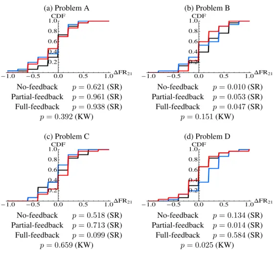
(a) Problem A (b) Problem B -1.0 -0.5 0.0 0.5 1.0DFR21 0.2 0.4 0.6 0.8 1.0CDF -1.0 -0.5 0.0 0.5 1.0DFR21 0.2 0.4 0.6 0.8 1.0CDF No-feedback p = 0.621 (SR) Partial-feedback p = 0.961 (SR) Full-feedback p = 0.938 (SR) p = 0.392 (KW) No-feedback p = 0.010 (SR) Partial-feedback p = 0.053 (SR) Full-feedback p = 0.047 (SR) p = 0.151 (KW) (c) Problem C (d) Problem D -1.0 -0.5 0.0 0.5 1.0DFR21 0.2 0.4 0.6 0.8 1.0CDF -1.0 -0.5 0.0 0.5 1.0DFR21 0.2 0.4 0.6 0.8 1.0CDF No-feedback p = 0.518 (SR) Partial-feedback p = 0.713 (SR) Full-feedback p = 0.099 (SR) p = 0.659 (KW) No-feedback p = 0.134 (SR) Partial-feedback p = 0.014 (SR) Full-feedback p = 0.584 (SR) p = 0.025 (KW)
Figure 2:Empirical cumulative distributions (CDF) of changes in relative frequencies of subject i who chose the better option between the 2nd block and the 1st block, i.e., ∆FR2,1. Black: no-feedback, Red: full-feedback, Blue:
partial-feedback. For each binary choice problem, the p-values for the within-treatment (one-tailed signed rank,SR) test and an across-treatment (Kruskal-Wallis, KW) test are reported below the panel corresponding to the choice problem.
Thus we have 30 observations of ∆FRil,m for each experimental condition.12 In this subsection, we focus on ∆FR2,1 and ∆FR8,1 in order to investigate whether different levels of payoff-related feedback have different impacts on subjects’ learning over both the short run and the long run.
For each binary choice problem, Figures 2 and 3 show the empirical cumulative distribution (CDFs) of ∆FR2,1and ∆FR8,1, respectively. Three colors correspond to the three feedback treat-ments: black is for no-feedback, red is for full-feedback, and blue is for partial-feedback. In each choice problem, the p-value for the one-tailed signed-rank (SR) test for each feedback treatment is reported below the panel corresponding to the choice problem, where the null hypothesis is ∆FR2,1 ≤ 0 (∆FR8,1 ≤ 0), and the alternative hypothesis is ∆FR2,1 > 0 (∆FR8,1> 0). Because
12
(a) Problem A (b) Problem B -1.0 -0.5 0.0 0.5 1.0DFR81 0.2 0.4 0.6 0.8 1.0CDF -1.0 -0.5 0.0 0.5 1.0DFR81 0.2 0.4 0.6 0.8 1.0CDF No-feedback p = 0.419 (SR) Partial-feedback p = 0.463 (SR) Full-feedback p = 0.281 (SR) p = 0.909 (KW) No-feedback p < 0.001 (SR) Partial-feedback p < 0.001 (SR) Full-feedback p < 0.001 (SR) p = 0.024 (KW) (c) Problem C (d) Problem D -1.0 -0.5 0.0 0.5 1.0DFR81 0.2 0.4 0.6 0.8 1.0CDF -1.0 -0.5 0.0 0.5 1.0DFR81 0.2 0.4 0.6 0.8 1.0CDF No-feedback p = 0.283 (SR) Partial-feedback p = 0.768 (SR) Full-feedback p < 0.001 (SR) p = 0.114 (KW) No-feedback p < 0.001 (SR) Partial-feedback p = 0.004 (SR) Full-feedback p = 0.218 (SR) p = 0.054 (KW)
Figure 3:CDFs of changes in relative frequencies of subject i who chose the better option between the 8th and the 1st block, i.e., ∆FR8,1. Black: no-feedback, Red: full-feedback, Blue: partial-feedback. For each binary choice problem,
the p-values for the within-treatment (one-tailed SR) test and an across-treatment (KW) test are reported below the panel corresponding to the choice problem.
we expect experience to enhance learning to choose the better option, we run a one-tailed test. The p-value for the Kruskal-Wallis (KW) test for a multiple comparison is also reported for each choice problem, where the null hypothesis is that the medians of ∆FR2,1 (∆FR8,1) are equal across the three feedback treatments.
For Problems A and C, ∆FR2,1 and ∆FR8,1were not significantly greater than zero for most of the feedback treatments except for ∆FR8,1 in the full-feedback treatment for Problem C. The absence of significant evidence of learning to choose the better option in Problems A and C is better understood in light of Observation 1. In Problems A and C, the subjects determined the better option as of Period 1 and they did not change their choices significantly in subsequent periods.
zero for most of the feedback treatments except ∆FR2,1in the partial-feedback treatment. Further, ∆FR2,1 was not significantly different across the three feedback treatments (p = 0.151, KW test). Thus, regardless of the feedback treatment, it seems that subjects learned to choose the better option more frequently (even in the first 10 periods) in Problem B. Comparing panels [b] in Figures 2 and 3, we see that, overall, the distributions of ∆FR8,1lie towards the right of those for ∆FR2,1, which implies that more subjects learned to choose the better option when they were given more time to learn.
In the case of Problem D, while ∆FR2,1 and ∆FR8,1 were not significantly greater than zero in the full-feedback treatment, they were both greater in the partial-feedback treatment. Our data do not make clear the reason for the absence of significant evidence of learning in the full-feedback treatment. In the no-feedback treatment, ∆FR8,1, but not ∆FR2,1, was significantly greater than zero, thus more subjects learned to choose the better option when they were given more time to learn.
Our observation for subjects’ learning can be summarized in the following way:
Observation 2. In Problem B and Problem D, subjects learn to choose the options with higher
expected payoffs even without any feedback information regarding their payoffs.
3.3 Meaningful learning (learning transfer)
In order to confirm “meaningful learning” in our data, we begin by comparing the percentage of inexperienced subjects in Period 1 and experienced subjects in Period 41 who chose the better option when they first encountered the same binary choice problem. Note that the experienced subjects faced a similar but different choice problem for the first 40 periods. Recall that the subjects faced one of the following sequences of binary choice problems in the order indicated by the arrows:
A → B, B → A, C → D, or D → C. Thus, for example, for Problem A we will compare
the choices made by inexperienced subjects in Period 1 with the choices made in Period 41 by experienced subjects who faced Problem B for the first 40 periods.
Table 3 presents the numbers of inexperienced subjects in Period 1 and experienced subjects in Period 41 who chose the better option for the three feedback treatments with the four binary choice problems. There are 30 subjects for each experimental condition defined by the sequence of problems and the feedback condition. The number of subjects who chose the better option in the pooled data (Pooled) is the sum of the number of subjects counted for the no-feedback (No-fb), partial-feedback (Partial-(No-fb), and full-feedback (Full-fb) treatments. The p-value for the χ2
Problem A Pooled (90) No-fb(30) Partial-fb (30) Full-fb (30) P-value (χ2)
Period 1 67 20 25 22 0.330
Period 41 48 15 16 17 0.967
p-value (χ2) 0.003 0.190 0.012 0.176
Problem B Pooled (90) No-fb(30) Partial-fb (30) Full-fb (30) P-value (χ2)
Period 1 31 9 13 9 0.455
Period 41 39 21 8 10 0.001
p-value (χ2) 0.221 0.002 0.176 0.781
Problem C Pooled (90) No-fb(30) Partial-fb (30) Full-fb (30) P-value (χ2)
Period 1 60 19 22 19 0.638
Period 41 64 23 22 19 0.495
p-value (χ2) 0.519 0.260 1.000 1.000
Problem D Pooled (90) No-fb(30) Partial-fb (30) Full-fb (30) P-value (χ2)
Period 1 22 8 5 9 0.457
Period 41 52 21 16 15 0.244
p-value (χ2) <0.001 <0.001 0.003 0.114
Table 3:Number of subjects who chose the better option. For each feedback treatment in each binary choice problem, there are a total of 30 subjects. The number of subjects who chose the better option in the pooled data (Pooled) is the sum of the number of subjects counted for the no-feedback (No-fb), partial-feedback (Partial-fb), and full-feedback (Full-fb) treatments. The p-values for χ2tests are reported for comparison across the three feedback treatments, and for comparisons between Periods 1 and 41. The subjects were faced with one of the following sequences of binary choice problems in the order indicated by arrows: A→ B, B → A, C → D, or D → C.
test is reported for all three feedback treatments and for the pooled data in each binary choice problem, where the null hypothesis is that the percentage of inexperienced subjects in Period 1 and experienced subjects in Period 41 who chose the better option are the same. The significantly more experienced subjects have chosen the better options than inexperienced subjects for no-feedback treatment in Problem B (p = 0.002) and for no-feedback and partial-feedback treatments in Problem D (p < 0.001 and p = 0.003, respectively). In Problem A, however, the percentage of experienced subjects who chose the better option was less than the percentage of inexperienced subjects for all three feedback treatments, which was statistically significant in the pooled data as well as in the partial-feedback treatment.
Thus, meaningful learning was observed for the no-feedback treatment in the sequence of Prob-lem A to ProbProb-lem B, as well as for the no-feedback and partial-feedback treatments for the sequence of Problem C to Problem D. Can we, however, say that this is truly significant evidence of
mean-ingful learning? Table 3 also reports, in the rightmost column, the results of χ2 test (p-values) for comparing the percentages across the three treatments. The null hypothesis here is that the percent-ages of subjects who chose the better option are equal across the three feedback treatments. With the exception of Period 41 in Problem B, there is no significant difference across the three feedback treatments in Period 41. The p-values for the χ2 test are 0.967, 0.001, 0.495, and 0.244 for Prob-lems A, B, C, and D, respectively. Therefore, we need to further verify whether different feedback treatments have different effects on subjects’ choices in the sequence of Problem C to Problem D.
For each experimental condition, we complement the above analysis by comparing the relative frequency in which inexperienced subject i chose the better option within the first block of 5 con-secutive periods (Periods 1 to 5), with the relative frequency in which experienced subject j chose the better option within the ninth block of 5 consecutive periods (Periods 41 to 45).
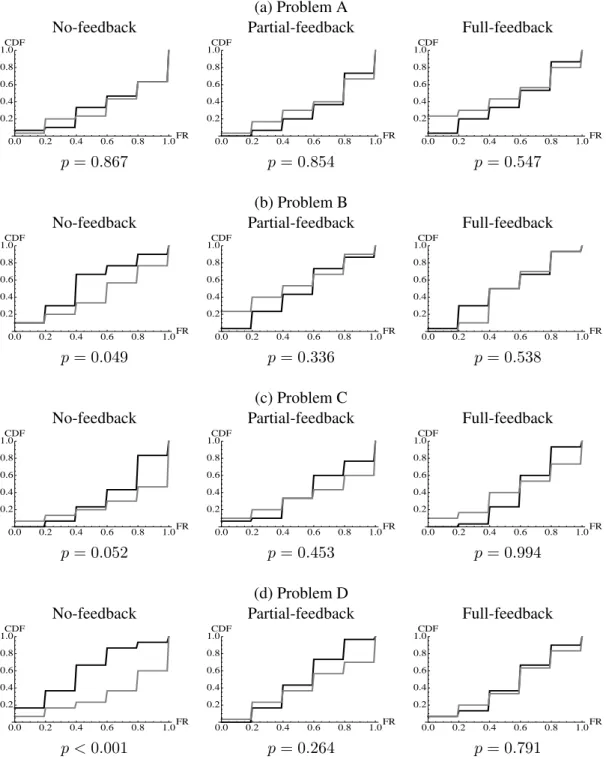
Figure 4 displays the distributions of FR1 (inexperienced subjects) in black and FR9 (experi-enced subjects) in gray for each feedback treatment in each binary choice problem. The p-value for the Mann-Whitney U-test (MW test) is reported under each panel which corresponds to a feed-back treatment for a binary choice problem, where the null hypothesis is FR1 = FR9. There were significant differences between FR1 and FR9 only for the no-feedback treatment in Problems B and D. (p = 0.049 and p < 0.001, respectively, MW test). We therefore discounted the case of partial-feedback treatment in Problem D as providing significant evidence of meaningful learning. Observation 3. Statistically significant evidence of meaningful learning was observed only for the
no-feedback treatment in Problem B and Problem D.
We found that withholding payoff-related feedback information stimulates meaningful learning in weighted voting games in the sense that experienced subjects have chosen the better option more frequently than inexperienced subjects when they faced the same problem. This is contrary to our prior expectation that the full-feedback treatment would be the most conducive for meaningful learning because subjects can observe how payoffs are equally distributed among the members of varying MWCs after each choice. The positive effect of withholding feedback on meaningful learning is, however, similar to what Rick and Weber (2010) found in the case of dominance solvable games.
(a) Problem A
No-feedback Partial-feedback Full-feedback
0.0 0.2 0.4 0.6 0.8 1.0FR 0.2 0.4 0.6 0.8 1.0CDF 0.0 0.2 0.4 0.6 0.8 1.0FR 0.2 0.4 0.6 0.8 1.0CDF 0.0 0.2 0.4 0.6 0.8 1.0FR 0.2 0.4 0.6 0.8 1.0CDF p = 0.867 p = 0.854 p = 0.547 (b) Problem B
No-feedback Partial-feedback Full-feedback
0.0 0.2 0.4 0.6 0.8 1.0FR 0.2 0.4 0.6 0.8 1.0CDF 0.0 0.2 0.4 0.6 0.8 1.0FR 0.2 0.4 0.6 0.8 1.0CDF 0.0 0.2 0.4 0.6 0.8 1.0FR 0.2 0.4 0.6 0.8 1.0CDF p = 0.049 p = 0.336 p = 0.538 (c) Problem C
No-feedback Partial-feedback Full-feedback
0.0 0.2 0.4 0.6 0.8 1.0FR 0.2 0.4 0.6 0.8 1.0CDF 0.0 0.2 0.4 0.6 0.8 1.0FR 0.2 0.4 0.6 0.8 1.0CDF 0.0 0.2 0.4 0.6 0.8 1.0FR 0.2 0.4 0.6 0.8 1.0CDF p = 0.052 p = 0.453 p = 0.994 (d) Problem D
No-feedback Partial-feedback Full-feedback
0.0 0.2 0.4 0.6 0.8 1.0FR 0.2 0.4 0.6 0.8 1.0CDF 0.0 0.2 0.4 0.6 0.8 1.0FR 0.2 0.4 0.6 0.8 1.0CDF 0.0 0.2 0.4 0.6 0.8 1.0FR 0.2 0.4 0.6 0.8 1.0CDF p < 0.001 p = 0.264 p = 0.791
Figure 4: CDFs of FR1(black) and FR9(gray) for the three feedback treatments with four binary choice problems:
no-feedback (left), partial-feedback (middle), and full-feedback (right). FR1is the relative frequency of periods in which
inexperienced subjects chose the better choice in the 1st block of 5 consecutive periods and FR9is the relative frequency
of periods in which subjects with experience of another problem chose the better option in the 9th block of 5 consecutive periods. The p-value for the Mann-Whitney U-test is reported for each feedback treatment in each binary choice problem.
4
Conclusion
By employing binary committee choice problems, this paper investigated whether withholding or varying feedback about the payoffs that resulted from subjects’ choices: (1) influenced subjects’ learning about the underlying relationship in weighted voting games between their nominal voting weights and their expected payoffs; and, (2) influenced the transfer of what subjects learned in one binary committee choice problem to a similar but different problem. To avoid possible complica-tions emerging from inexperienced subjects simultaneously learning to play weighted voting games, we drastically simplified the experimental design so that instead of letting subjects play weighted voting games, we made subjects choose one of two committees (two weighted voting games) in a binary committee choice problem. In our binary committee choice problems, the payoffs for sub-jects after each choice were generated stochastically based on a theory proposed by Deegan and Packel (1978). Subjects were told that the payoffs were mechanically generated based on a theory of decision making in committees but were not given the details of the exact theory being used.
Our main findings are as follows: (1) subjects learned to choose the committee that generated higher expected payoffs even without any immediate feedback information on the payoffs received as a result of their choices; and (2) statistically significant evidence of meaningful learning was observed only for the treatment with no payoff-related feedback information. Our findings support the positive effect of withholding immediate payoff feedbacks in promoting “meaningful learning” that Rick and Weber (2010) found in some dominance solvable games.
Well-known models of learning, such as the reinforcement learning, belief-based learning, or EWA learning models, do not make any predictions about whether learning takes place when there is no feedback related to payoffs. This is also the case for more recently proposed models of learning such as “individual evolutionary learning.” Our finding calls for a new class of models of learning that allow for learning based on introspection. Furthermore, when it comes to modeling “meaningful learning,” it seems essential to create an explicit formalization of the process of introspection that includes a means of assessing how varying feedback stimulates or hinders this type of learning. Such theoretical developments will guide us in designing experiments to clarify issues such as for which classes of games does withholding immediate payoff-related feedback stimulate subjects’ learning. We believe this to be a fruitful avenue for future research.
References
ALESKEROV, F., A. BELIANIN, ANDK. POGORELSKIY(2009): “Power and preferences: an ex-perimental approach,” Available at SSRN: http://ssrn.com/abstract=1574777.
ARIFOVIC, J. ANDJ. LEDYARD(2012): “Individual evolutionary learning, other-regarding prefer-ences, and the voluntary contributions mechanism,” Journal of Public Economics, 96, 808–823. ARIFOVIC, J., R. D. MCKELVEY, AND S. PEVNITSKAYA(2006): “An initial implementation of
the Turing tournament to learning in two person games,” Games and Economic Behavior, 57, 93–122.
BANKS, J., M. OLSON, AND D. PORTER (1997): “An experimental analysis of the bandit
prob-lem,” Economic Theory, 10, 55–77.
BANZHAF, J. F. (1965): “Weighted voting doesn’t work: a mathematical analysis,” Rutgers Law
Review, 19, 317–343.
CAMERER, C.AND T.-H. HO (1999): “Experience-weighted attraction learning in normal form
games,” Econometrica, 67, 827–874.
CASON, T. N.ANDD. FRIEDMAN(1997): “Price formation in single call markets,” Econometrica, 65, 311–345.
CHEUNG, Y.-W. AND D. FRIEDMAN(1997): “Individual learning in normal form games: some laboratory results,” Games and Economic Behavior, 19, 46–76.
COOPER, D. J.AND J. H. KAGEL(2003): “Lessons learned: generalized learning across games,”
American Economic Review, Papers and Proceedings, 93, 202–207.
——— (2008): “Learning and transfer in signaling games,” Economic Theory, 34, 415–439. DEEGAN, J.ANDE. PACKEL(1978): “A new index of power for simple n-person games,”
Interna-tional Journal of Game Thoery, 7, 113–123.
DROUVELIS, M., M. MONTERO,ANDM. SEFTON(2010): “The paradox of new members: strate-gic foundations and experimental evidence,” Games and Economic Behavior, 69, 274–292. DUFWENBERG, M., R. SUNDARAM, ANDD. J. BUTLER(2010): “Epiphany in the Game of 21,”
EREV, I., E. ERT, AND A. E. ROTH (2010): “A choice prediction competition for market entry games: an introduction,” Games, 2, 117–136.
EREV, I. AND A. E. ROTH (1998): “Predicting how people play games: reinforcement learning in experimental games with unique, mixed strategy equilibria,” American Economic Review, 88, 848–81.
ESPOSITO, G., E. GUERCI, X. LU, N. HANAKI, AND N. WATANABE (2012): “An experimental study on “meaningful learning” in weighted voting games,” Mimeo, Aix-Marseille University. FELSENTHAL, D. S. AND M. MACHOVER (1998): The Measurement of Voting Power : Theory
and Practice, Problems and Paradoxes, London: Edward Elgar.
FISCHBACHER, U. (2007): “z-Tree: Zurich toolbox for ready-made economic experiments,”
Ex-perimental Economics, 10, 171–178.
FRECHETTE´ , G. R., J. H. KAGEL, AND M. MORELLI (2005a): “Gamson’s law versus non-cooperative bargaining theory,” Games and Economic Behavior, 51, 365–390.
——— (2005b): “Nominal bargaining power, selection protocol, and discounting in legislative bargaining,” Journal of Public Economics, 89, 1497–1517.
GUERCI, E., N. HANAKI, N. WATANABE, X. LU,ANDG. ESPOSITO(2014): “A methodological note on a weighted voting experiment,” Social Choice and Welfare, 43, 827–850.
HANAKI, N., R. SETHI, I. EREV, AND A. PETERHANSL(2005): “Learning strategy,” Journal of
Economic Behavior and Organization, 56, 523–542.
HART, S. (2005): “Adaptive heuristics,” Econometrica, 73, 1401–1430.
HARUVY, E. AND D. O. STAHL (2009): “Learning transference between dissimilar symmetric normal-form games,” Mimeo, University of Texas at Dallas.
——— (2012): “Between-game rule learning in dissimilar symmetric normal-form games,” Games
and Economic Behavior, 74, 208–221.
HO, T.-H., C. CAMERER, AND K. WEIGELT (1998): “Iterated dominance and iterated best re-sponse in experimental “p-beauty contests”,” American Economic Review, 88, 947–969.
HU, Y., Y. KAYABA, AND M. SHUM(2013): “Nonparametric learning rules from bandit experi-ments: The eyes have it!” Games and Economic Behavior, 81, 215–231.
IOANNOU, C. A.AND J. ROMERO(2014): “A generalized approach to belief learning in repeated games,” Games and Economic Behavior, 87, 178–203.
KAGEL, J. H., H. SUNG, ANDE. WINTER(2010): “Veto power in committees: an experimental study,” Experimental Economics, 13, 167–188.
MARCHIORI, D. AND M. WARGLIEN (2008): “Predicting human interactive learning by regret-driven neural networks,” Science, 319, 1111–1113.
MEYER, R. J. ANDY. SHI(1995): “Sequential choice under ambiguity: intuitive solutions to the
armed-bandit problem,” Management Science, 41, 817–834.
MONTERO, M., M. SEFTON,AND P. ZHANG(2008): “Enlargement and the balance of power: an experimental study,” Social Choice and Welfare, 30, 69–87.
NEUGEBAUER, T., J. PEROTE, U. SCHMIDT, ANDM. LOOS(2009): “Selfish-baised conditional cooperation: on the decline of contributions in repeated public goods experiments,” Journal of
Economic Psychology, 30, 52–60.
RICK, S. AND R. A. WEBER (2010): “Meaningful learning and transfer of learning in games
played repeatedly without feedback,” Games and Economic Behavior, 68, 716–730.
SHAPLEY, L. S.AND M. SHUBIK(1954): “A method for evaluating the distribution of power in a committee system,” American Political Science Review, 48, 787–792.
——— (1966): “Quasi-cores in a monetary economy with non-convex preferences,” Econometrica, 34, 805–827.
SPILIOPOULOS, L. (2012): “Pattern recognition and subjective belief learning in a repeated constant-sum game,” Games and Economic Behavior, 75, 921–935.
——— (2013): “Beyond fictitious play beliefs: Incorporating pattern recognition and similarity matching,” Games and Economic Behavior, 81, 69–85.
STAHL, D. O. (1996): “Boundedly rational rule learning in a guessing game,” Games and Economic
Appendix
Instructions
You will be asked to repeatedly make a simple choice between two options.
Imagine that you need to represent your interests within a voting committee. This committee decides how to divide 120 points among its members. The committee has three other members, and each member has a predetermined number of votes, which may be different from one to the other. The committee will make a decision only when a proposal receives the pre-determined required number of votes. You will be told what is the required number of votes. If more than one proposal is put before the committee, the members cannot vote for multiple proposals by dividing their allocated number of votes. A member can vote for only one proposal, and all of his/her votes must be cast for that proposal.
You are asked to choose which of the two possible committees you prefer to join. You will be informed of the number of votes allocated to each of the four members of the committee (including you), and the number of votes required for a proposal to be approved. The number of votes you have will always be indicated with the label YOU.
Full-feedback treatment
There is a total of 60 periods. In each period, you have 30 seconds to make your choice between the two committees. If you do not make a choice within the 30 seconds in one period, you will receive zero points for that period. When a choice is made, the chosen committee will automatically allocate 120 points among the four members. The outcomes may vary from one period to another, but are based on a theory of decision making in committees. Once the allocation is made, you will immediately be shown the resulting allocation. At the end of the experiment, you will be paid according to your total earnings during the 60 periods, at an exchange rate of 1 point = JPY1.
If you have any questions, please raise your hand.
No-feedback treatment
There is a total of 60 periods. In each period, you have 30 seconds to make your choice between the two committees. If you do not make any choice within the 30 seconds in one period, you will receive zero points for the period. When a choice is made, the chosen committee will automatically
allocate 120 points between the four members. The outcomes may vary from one period to another, but they are based on a theory of decision making in committees. You will not see the resulting allocation after each period. However, at the end of the experiment, you will be told the total points you have obtained during the 60 periods, and you will be paid according to the points earned over the 60 periods at an exchange rate of 1 point = JPY1.
If you have any questions, please raise your hand.
Partial-feedback treatment
There is a total of 60 periods. In each period, you have 30 seconds to make your choice between the two committees. If you do not make any choice within the 30 seconds in one period, you will receive zero points for the period. When a choice is made, the chosen committee will automatically allocate 120 points among the four members. The outcomes may vary from one period to another, but they are based on a theory of decision making in committees. Once the allocation is made, you will be shown the number of points allocated to you. You will not see the allocations to the other members of the committee. At the end of the experiment, you will be paid according to your total points score at an exchange rate of 1 point = JPY1.