Publisher’s version / Version de l'éditeur:
Vous avez des questions? Nous pouvons vous aider. Pour communiquer directement avec un auteur, consultez la première page de la revue dans laquelle son article a été publié afin de trouver ses coordonnées. Si vous n’arrivez pas à les repérer, communiquez avec nous à PublicationsArchive-ArchivesPublications@nrc-cnrc.gc.ca.
Questions? Contact the NRC Publications Archive team at
PublicationsArchive-ArchivesPublications@nrc-cnrc.gc.ca. If you wish to email the authors directly, please see the first page of the publication for their contact information.
https://publications-cnrc.canada.ca/fra/droits
L’accès à ce site Web et l’utilisation de son contenu sont assujettis aux conditions présentées dans le site LISEZ CES CONDITIONS ATTENTIVEMENT AVANT D’UTILISER CE SITE WEB.
Energy Science & Engineering, 7, 6, pp. 2498-2509, 2019-12-17
READ THESE TERMS AND CONDITIONS CAREFULLY BEFORE USING THIS WEBSITE. https://nrc-publications.canada.ca/eng/copyright
NRC Publications Archive Record / Notice des Archives des publications du CNRC :
https://nrc-publications.canada.ca/eng/view/object/?id=b862804c-c13e-40f7-8d31-f6985edcf7a2 https://publications-cnrc.canada.ca/fra/voir/objet/?id=b862804c-c13e-40f7-8d31-f6985edcf7a2
Archives des publications du CNRC
This publication could be one of several versions: author’s original, accepted manuscript or the publisher’s version. / La version de cette publication peut être l’une des suivantes : la version prépublication de l’auteur, la version acceptée du manuscrit ou la version de l’éditeur.
For the publisher’s version, please access the DOI link below./ Pour consulter la version de l’éditeur, utilisez le lien DOI ci-dessous.
https://doi.org/10.1002/ese3.438
Access and use of this website and the material on it are subject to the Terms and Conditions set forth at
Numerical investigations of a novel vertical axis wind turbine using
blade element theory
-vortex filament method (BET-VFM)
Hilewit, Doma; Matida, Edgar; Fereidooni, Amin; Abo el Ella, Hamza;
Nitzsche, Fred
2498
|
wileyonlinelibrary.com/journal/ese3 Energy Sci Eng. 2019;7:2498–2509.1
|
INTRODUCTION
World energy generation (including renewable and nonrenew-able sources) should increase ~28% by 2040,1 when the
con-tribution from renewable sources (wind, solar, hydropower, geothermal, and others) would increase to at least 31% of the total energy production, mainly from wind and solar power generation expansions. Wind energy (including offshore ap-plications) is currently responsible for more than 40% of the total renewable energy growth. Horizontal axis wind turbines (HAWTs), which need to stand on massive concrete or steel
towers, exhibited a number of drawbacks for deep‐water off-shore applications if anchored to depths >40 m.2-5 Vertical
axis wind turbines (VAWT), on the other hand, could poten-tially be installed offshore 6 (mainly in deeper waters using
floating platforms, eg, DEEPWIND.EU project).
VAWT have been divided into three categories: Darrieus troposkein, H‐Darrieus, and Savonius rotor. The troposkein de-sign has curved blades (similar to an egg beater). This shape was proposed by G. Darrieus in 1931.7 Although the troposkein
rotor‐based design was the most sophisticated turbine among several other VAWT designs, it has not been widely explored
R E S E A R C H A R T I C L E
Numerical investigations of a novel vertical axis wind turbine
using Blade Element Theory‐Vortex Filament Method
(BET‐VFM)
Doma Hilewit
1|
Edgar Matida
1|
Amin Fereidooni
2|
Hamza Abo el Ella
2|
Fred Nitzsche
1This is an open access article under the terms of the Creative Commons Attribution License, which permits use, distribution and reproduction in any medium, provided the original work is properly cited.
© 2019 The Authors. Energy Science & Engineering published by the Society of Chemical Industry and John Wiley & Sons Ltd.
1Department of Mechanical and Aerospace Engineering, Carleton University, Ottawa, ON, Canada
2National Research Council Canada, Ottawa, ON, Canada
Correspondence
Doma Hilewit, Department of Mechanical and Aerospace Engineering, Carleton University, 1125 Colonel By Drive, Ottawa, ON, K1S 5B6, Canada.
Email: domahilewit@cmail.carleton.ca
Abstract
The aerodynamic performance of three different configurations of vertical axis wind turbines (VAWT), namely: (a) conventional Darrieus troposkein VAWT (based on turbines designed by Sandia National Laboratories), (b) novel 50% STS‐VAWT (50% shifted‐troposkein‐shaped STS‐VAWT), and (c) novel 100% STS‐VAWT were investigated numerically. An in‐house code, which combined the blade ele-ment theory (BET) and the vortex filaele-ment method (VFM), was used. The main purpose of this work was to develop an aerodynamic code to predict the performance of conventional VAWT as well as assess the novel 50% and 100% STS‐VAWT con-figurations. Simulation results (power coefficients) were verified and then validated against experimental data available from the literature (2‐, 5‐, and 17‐m conventional troposkein VAWT measured by Sandia National Laboratories). Additional numeri-cal results showed that the 50% STS‐VAWT outperformed both the conventional VAWT and the 100% STS‐VAWT by up to 14% (peak power), within the range of rotation and turbine sizes that were investigated in the present work.
K E Y W O R D S
in the past due to some drawbacks, including lower aerody-namic performance when compared against HAWTs. One of the sources of lower performance was attributed to blade‐tex interactions (BVIs) between the downwind blades with vor-tices (and wake) generated by the upwind blades during normal turbine operation. The effects of BVI also increased the aero-dynamic cyclic stresses on the blades, thus increasing blade fatigue, leading to premature failure. The BVI effects strongly depend on the tip‐speed ratio (TSR, the ratio of the blade veloc-ity at the equator of the turbine to the wind velocveloc-ity). This has been verified experimentally by Fujisawa and Shibuya,8 who
described the shedding of two pairs of vortices that leave the vicinity of the blades for different tip‐speed ratios.
To overcome the performance limitations of the conven-tional troposkein VAWT, a novel configuration has been proposed by the present authors,9 mainly by trying to reduce
the negative impact of the BVI on the turbine blade of the conventional troposkein VAWT (see Figure 1A). As shown in Figure 1B, C, a shifted‐troposkein shape vertical axis wind turbine (STS‐VAWT) has been presented, where the height and frontal area of each blade were decreased and shifted vertically with respect to the other blade. The swept area was kept constant for comparison purposes. As the result of this shift, the second blade does not exactly follow the path of the other advancing blade; a path which is continuously dis-turbed by vortices generated by the advancing blade, a fact that should improve performance, as discussed later.
Regardless of the category, all Darrieus VAWT have similar complexities related to their unsteady aerodynamic behavior. Since the VAWT blades revolve around its axis of rotation, the rotation velocity and the wind velocity, in addi-tion to the induced velocity from vortices generated by the blades, all combine to produce a velocity vector that changes the angle of attack (thus lift and drag forces) of the flow over the blades at each azimuthal direction (rotation angle). The vortices are generated and shed by the blades with the same circulation strength as the variation of lift in time. The com-plexity of this unsteady aerodynamics makes the accurate prediction of VAWT performance a challenging problem.
Various aerodynamic models have been developed to pre-dict and analyze the aerodynamic loads and performance of wind turbines. Using single or multiple streamtubes, in addi-tion to the streamwise momentum equaaddi-tion, initial simplified models were able to predict the overall power output and aero-dynamic forces around the VAWT blades.10,11 A
double‐mul-tiple streamtube model was described by Paraschivoiu,12 but
underperformed during high tip‐speed ratios or high solidity conditions.7,11 These initial models (not fully representing the
physics of the problem) led to the development of the vor-tex filament method by Strickland and coworkers 13 to
simu-late the complex interactions between the three‐dimensional wake flow and the turbine blades. In their work, the VAWT performance was simulated by dividing the blade into several
spanwise elements, each element replaced by a lifting line with a bound circulation. The bound vortex strength at each element was evaluated in time using empirical aerodynamic information at a certain angle of attack (blade element theory, BET), which was determined from the blade rotation, free stream velocity, and wake vortex filaments that were shed and tracked in time (ie, the vortex filament method, VFM). The change in circulation around each element of the blade in time was obtained using the Kutta‐Joukowski theorem. VFM is gridless and represents an approximation technique to solve unsteady, incompressible, Navier‐Stokes equations using vorticity transport equations. The vorticity field can be obtained from the combination of vortex filament elements tracked in a Lagrangian frame of reference. Scheurich and co-workers 14,15 adopted this BET/VFM approach and predicted
the performance of three different configurations of VAWT: H‐Darrieus, troposkein Darrieus, and a helical structure, under steady and unsteady wind conditions. Their simulation results exhibited reasonable agreement with the experimental data and provided a valuable representation of the near wake profile.
In the present work, an in‐house code using the BET‐ VFM (blade element theory‐vortex filament method) ap-proach proposed by Strickland et al13 was developed and
validated against conventional troposkein VAWT data (power coefficients) available in the literature (Sandia National Laboratories; turbines with diameters and heights of ~2‐, 5‐, and 17‐m). The power coefficients of two ad-ditional novel geometries (50% STS‐VAWT, and 100% STS‐VAWT, refer again to Figure 1B, C) were simulated for three different turbine sizes (2‐, 5‐, and 17‐m) using the BET‐VFM validated code.
2
|
IMPLEMENTATION OF THE
PRESENT IN‐HOUSE MATLAB CODE
The following steps outline the numerical procedures (based on Strickland et al13 and Fereidooni16), which wereimple-mented into the in‐house code. In the first step, the turbine blades were divided into a number of spanwise elements (blade sections), as shown in Figure 2A (the element at the equator of a blade is enlarged for the sake of clarity in the figure). A local coordinate system is also defined and placed at the aerodynamic center of the airfoil (Figure 2B).
The relative velocity, UR
(i,j), as seen by each element is given by the following relation:
where subscripts i and j denote element number and time
step, respectively. (U, V, W) is the velocity vector induced on the blade element by the wake behind the blades (obtained (1)
from the contribution of all vortex filaments that are shed and tracked in time), Ut= Ri𝜔 is the element rotational velocity, Ri
is the element radius of rotation, 𝜔 is the element angular
ve-locity, U∞ is the freestream (wind) velocity, 𝜃 is the azimuth
(rotational) angle, and i, j, and k are unit vectors following a
fixed Cartesian coordinate system.
The angle of attack of the flow against the blade element
𝛼(i,j) can be obtained from the relative flow velocity vector as
seen by the element, or Equation 1. After obtaining this angle of attack, the element lift coefficient per unit span (Cl
(i,j)) as well as drag coefficient per unit span (Cd
(i,j)) can be obtained (using linear interpolation) from airfoil experimental data at different Reynolds numbers and angles of attack.17,18 The
tangential and normal coefficients (as well as respective forces) acting on the blade element can be obtained from the lift and drag coefficients by
Each element at a particular time was associated with a single bound vortex strength Γb
(i,j) and defined as
where Cl
(i,j) is the lift coefficient per unit span and c is the airfoil chord length. Notice that the magnitude of the relative
flow velocity around the blade element is approximated as the average velocity between the values at the two spanwise ends of the element.
As a consequence of changing the angle of attack on the blade in time (due to rotation), the lift and the bound vor-tex strength will also change accordingly. This change in the bound vortex strength results in the shedding of a spanwise vortex at the trailing edge of an element at a certain time step, while keeping the change of the total circulation, Γ, equal to
zero, by following Kelvin's circulation theorem
The shed bound vortex circulation strength from an ele-ment in time, Γs
(i,j), is given by
In order to numerically represent the change in bound vortex strength along the blade elements, trailing vortices perpendicular to the trailing edge must also be shed with the following circulation strength
The shedding of vortex filaments (three time steps) was also depicted in Figure 2 for the enlarged element at the equator. All spanwise elements will also shed vortex fila-ments in a similar way. The Adams‐Bashforth integration method 19 was used to calculate and update the positions
(2)
Ct
(i,j)= Cl(i,j) sin 𝛼(i,j)− Cd(i,j) cos 𝛼(i,j)
(3)
Cn
(i,j)= Cl(i,j) cos 𝛼(i,j)+ Cd(i,j) sin 𝛼(i,j)
(4)
Γb
(i,j)=
1
2Cl(i,j)c(|UR(i,j)| + |UR(i+1,j)|)∕2
(5)
DΓ
Dt = 0
(6)
Γs
(i,j)= Γb(i,j)− Γb(i,j−1)
(7)
Γt
(i,j)= Γb(i+1,j)− Γb(i,j)
FIGURE 1 Geometries used in the current work: A, Conventional B, 50% STS C, 100% STS. Same turbine height, H, and same swept area, As
of these vortex filaments in time. Each vortex filament is allowed to stretch and rotate while being convected in the flow field. Each vortex filament will also induce a velocity,
Vind, at a particular point, P, as shown in Figure 3. All
fila-ments will contribute to the induced velocity vector (U, V,
W) in Equation 1) by means of the Biot‐Savart Law, which
can be written as
The dimensionless power coefficient for the turbine can be obtained from the summation of the contributions of all elements along the blades in time using
where P is the average power generated by the turbine in time,
Q(i,j) is the torque generated by a blade element at a particular
time (the element torque is obtained from the product of the element tangential force and the element rotation radius), 𝜌 is
the fluid density, As is the swept area (total frontal area of the
revolving turbine), NT is the number of the time steps, NE is the number of blade elements, and 𝜔 is the blade angular velocity.
Subscripts i and j denote element number and time step,
respec-tively, as described before. Separate analysis (using 5, 10, 15, and 20 revolutions) indicated that power coefficient results (at different tip‐speed ratios, varying from 2.5 to 10.5) for 15 full blade revolutions are nearly identical to 20 full blade revolution results, indicating adequate convergence when 15 revolutions are used in the present simulations. The tip‐speed ratio (TSR or
𝜆) is defined as
where R is the maximum radius of rotation of the turbine.
3
|
TURBINE CONFIGURATIONS
This paper specifically describes the performance comparisons (in terms of power coefficients) between the novel configura-tion design (STS‐VAWT) configuraconfigura-tions and the convenconfigura-tional design of troposkein VAWT. To ensure a consistent compari-son, the geometry of each configuration modeled has two blades curved as per the Sandia design, with a constant NACA four‐ digit airfoil cross section along the blade. The turbine height‐ to‐diameter ratio of each configuration is selected as one. The height of the turbine, H, the aspect ratio AR = H/D, and the swept area are fixed when comparisons between turbines are performed. Several aspects of each rotor configurations are pre-sented in the following subsections.
3.1
|
Conventional configuration
The Sandia National Laboratories tested three conventional troposkein VAWT with approximate diameters of 2, 5, and 17‐m,20-23 as illustrated in Figure 4. The power generated by
each turbine was measured at different wind speeds while the rotation was maintained constant. Each of these turbines consisted of two blades with three segments: a circular arc located at the turbine equator, and two straight sections that are attached to the circular arc and to the main shaft (result-ing in a practical simplification of the troposkein curve). The current numerical work uses exactly the same three ge-ometries and experimental conditions as the ones proposed by Sandia for the conventional troposkein VAWT. Table 1 summarizes and defines several parameters that describe the shape of the conventional VAWT, including the rotor solid-ity 𝜎= N c l∕As, the chord‐to‐radius ratio, c/R, the chord‐to‐
length ratio, c/l, and the rotor aspect ratio AR = H/D. N, c, l
, and As are the number of blades, airfoil chord length, blade
length, and the swept area (total frontal projection area of the revolving turbine, see again 1), respectively. R is the
maxi-mum radius of rotation, D= 2R is the maximum diameter of
rotation, and H is the turbine height.
(8) Vind=Γv 4𝜋 ∫ r× dl |r|3 = Γv 4𝜋 r1× r2 |r1× r2|2 (r 0⋅ r1 |r1| −r0⋅ r2 |r2| ) (9) Cp= P 1 2As𝜌U 3 ∞ = 1 NT NT ∑ j=1 NE ∑ i=1 Q(i,j)𝜔 1 2As𝜌U 3 ∞ (10) 𝜆= 𝜔R U∞ FIGURE 2 Blade elements (sections) and vortex filaments along with A, global coordinate system and B, local coordinate system (placed at 1/4 chord)
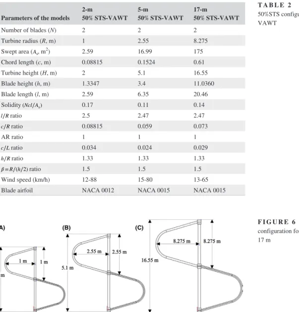
3.1.1
|
50% STS configuration
Figure 5 and Table 2 show the details of the 50% STS‐VAWT geometry used here. Each turbine (2‐, 5‐, and 17‐m) has the same height and swept area as the respective conventional VAWT shown previously in Figure 4. The main modifica-tions that were made to the 50% STS‐VAWT configuramodifica-tions for the three diameters were as follows:
• Turbine blade heights were decreased by 33.3% with re-spect to the conventional.
• Turbine blade lengths of 2‐, 5‐, and 17‐m turbines were decreased by 12.79%, 15.67%, and 15.7%, respectively. • 𝛽 ratios, which is the ratio of the maximum blade
displace-ment from the axis of rotation to half of the blade height,18
was increased from 1 to 1.5.
• l∕R ratios of 2‐m, 5‐m, and 17‐m based design turbines
were decreased by 13.7%, 14.8%, and 14.8%, respectively.
3.1.2
|
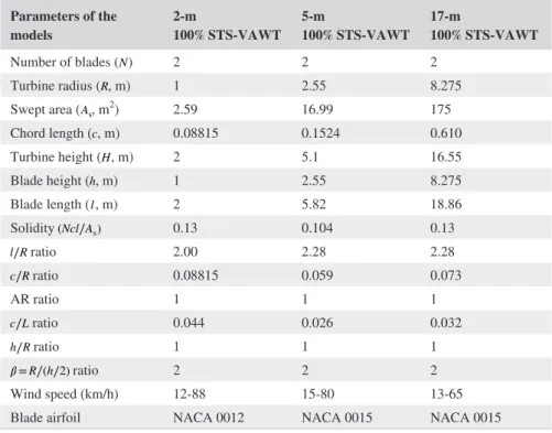
100% STS configuration
Figure 6 and Table 3 show the details of the 100% STS‐ VAWT geometry used here. The main modifications that were made to the 100%STS‐VAWT configurations for the three diameters were as follows:
• Turbine blade heights were decreased by 50% with respect to the conventional one.
• Turbine blade lengths of 2‐, 5‐, and 17‐m turbines were decreased by 32.6%, 22.7%, and 22.3%, respectively. • 𝛽 ratios were increased from 1 to 2.
• l∕R ratio of 2‐m, 5‐m, and 17‐m turbines were decreased
by 31.03%, 21.3%, and 21.3%, respectively.
4
|
RESULTS AND DISCUSSION
4.1
|
Numerical validation against
conventional VAWT
Prior to the final numerical analysis of the performance of the VAWT, it was vitally important to verify whether the simulations were fully converged. Initially, 23 and 47 uniform blade elements were used in the spatial discretiza-tion, showing nearly identical power coefficient results in the current simulations. It was also essential to investigate the effects of the simulation time step (shown in terms of azimuth angle increments of the rotational blade; smaller increments indicating smaller time steps) on the resulted maximum power coefficient of each conventional tropo-skein VAWT, as shown in Figure 7. From the results, no considerable change in peak power is observed for angle increments below 15°. Thus, an angle increment (represent-ing a time step) of 15° has been adopted for all remain(represent-ing
simulations, in addition to 23 blade elements (spatial reso-lution) and 15 full blade revolutions (total simulation time as indicated before), all giving adequate spatial and tem-poral resolutions when power coefficient simulations are concerned. For a single simulation of a particular turbine, a rotational velocity and a wind speed are selected, and then, the power coefficient is obtained after 15 turbine revolu-tions. Other wind speeds are selected while the rotational speed is maintained constant and the procedure to obtain the power coefficient is repeated for each wind speed. The effects of the blade ends (tip vortices) as well as the effects of the shaft and struts on the turbine performance were as-sumed to be negligible for the current turbines (since the shaft‐to‐turbine diameter ratio would be relatively small) and were therefore not modeled in current work, but should be further investigated in future work.
Simulation predictions (using the in‐house MATLAB code) of the performance (CP− 𝜆) of the three conventional
VAWT configurations (2‐, 5‐, 17‐m) were validated against test data from the Sandia National Laboratories found in the literature 20-22 as well as other aerodynamic code results.7,24
The experimental power coefficient of Sandia 2‐meter was plotted versus tip‐speed ratio (CP− 𝜆) in Figure 8A, together
with current simulation prediction results. It can be seen in this figure that the current aerodynamic model showed good agreement, particularly at a TSR beyond the peak power for
𝜆≥ 4.3, whereas some discrepancies were obtained in the
lower tip regions (𝜆≥ 4.0). This could be justified by the fact
that the airfoil coefficient values (Cl and CD) from the used
database were less accurate at low Reynolds number (due to data sparsity and linear interpolation). In Figure 8B, the power coefficient curve of Sandia 5‐m VAWT was predicted by DMST (double‐multiple stream tube) model, MST (mul-tiple stream tube) model, and the present model. The differ-ences between the predictions of the two previous models and the experimental data were significant, particularly at high range of TSR (𝜆≥ 4.5), whereas the present model
re-sults agreed relatively well with the experimental data over a wide range of tip‐speed ratio, despite a slight overprediction
FIGURE 3 Induced velocity at a point P from a vortex filament of strength, Γv
of peak power and underprediction of power coefficients for low tip‐speed ratios (𝜆≤ 3.0). Fidelity higher than DMST and
MST can be achieved using CFD (computational fluid dy-namics) 25,26 techniques, but direct comparison could not be
performed in the present work.
Figure 8C depicts the final comparison between the pres-ent code (in‐house MATLAB code) and the experimpres-ental data of Sandia 17‐m, but this time they were compared with
predictions made with three different aerodynamic codes, as reported by Touryan et al24 As the scale of the turbine
increased (turbine size), the Reynolds numbers increased, which led to an improvement over the blade performance in general. Here, although all models performed well, the present simulation results seem to have an overall good agreement against the experimental data over a wide range of tip‐speed ratio. Except for small tip‐speed ratios (𝜆≤ 2.5 FIGURE 4 Conventional VAWT
configuration for A, 2 m, B, 5 m, and C, 17 m
Parameters of the
models 2‐m VAWT 5‐m VAWT 17‐m VAWT
Number of blades (N) 2 2 2 Turbine radius (R, m) 1 2.55 8.275 Swept area (As, m2) 2.59 16.99 175 Chord length (c, m) 0.08815 0.1524 0.61 Turbine height (H, m) 2 5.10 16.55 Blade height (h, m) 2 5.10 16.55 Blade length (l, m) 2.97 7.5300 24.273 Solidity (Ncl/As) 0.2 0.13 0.16 l/R ratio 2.9 2.9 2.9 c/R ratio 0.08815 0.059 0.073 AR ratio 1 1 1 c∕L ratio 0.029 0.020 0.025 h∕R ratio 2 2 2 𝛽= R∕(h∕2) ratio 1 1 1 Wind speed (km/h) 12‐88 15‐80 13‐65
Blade airfoil NACA 0012 NACA 0015 NACA 0015
TABLE 1 Specifications of the conventional configuration of DOE‐Sandia VAWT
FIGURE 5 50% STS‐VAWT configuration for A, 2 m, B, 5 m, and C, 17 m
), the current numerical results slightly overpredict the ex-perimental values.
4.2
|
Aerodynamic performance of the
turbine models
A comparison of the power coefficients as function of the tip‐speed ratio between the simulation results for the 2‐m conventional troposkein VAWT (light gray line), 2‐m 50% STS‐VAWT (black line), and 2‐m 100% STS (dark gray line), and the Sandia experimental data (circle symbols) is shown in Figure 9. Despite smaller solidity, the superior performance of 50% STS‐VAWT against the conventional troposkein VAWT was expected due to less blade‐vortex interactions (BVIs), in this case, interactions between the wake vortices generated by the advancing blade and the power producing section of the second blade, as discussed before. Notice, how-ever, that even though experiencing the least amount of BVIs when compared to the other two configurations, the 100%
STS model produced the least amount of peak power. This is likely due to geometry constrictions, since the 100% STS‐ VAWT has also the smallest power producing blades, also reflected by the lowest solidity 𝜎, higher 𝛽 ratio, and smaller
blade height when compared to the 50% STS‐VAWT. These aspects were known to have negative impacts on the aero-dynamic performance as reported before.20 Results suggest
that the peak power is a compromise between BVI reduction and solidity. When the turbine rotation speed is increased from 267 to 400 rpm, the BVI effect becomes more prevalent since the blade wake would stay in the blade's path for sev-eral revolutions. Consequently, the generated aerodynamic performance of the 50% STS‐VAWT increased and peaked at higher tip‐speed ratio of 𝜆 = 7.6 (see Figure 9B). Although
the 100% STS‐VAWT slightly outperformed the conven-tional troposkein VAWT and the 50% STS‐VAWT for low tip‐speed ratios (𝜆≤ 4.0), it underperformed against the 50%
STS‐VAWT for higher and more relevant (in terms of power producing) TSRs.
Parameters of the models 2‐m50% STS‐VAWT 5‐m50% STS‐VAWT 17‐m50% STS‐VAWT
Number of blades (N) 2 2 2 Turbine radius (R, m) 1 2.55 8.275 Swept area (As, m2) 2.59 16.99 175 Chord length (c, m) 0.08815 0.1524 0.61 Turbine height (H, m) 2 5.1 16.55 Blade height (h, m) 1.3347 3.4 11.0360 Blade length (l, m) 2.59 6.35 20.46 Solidity (Ncl∕As) 0.17 0.11 0.14 l∕R ratio 2.5 2.47 2.47 c∕R ratio 0.08815 0.059 0.073 AR ratio 1 1 1 c∕L ratio 0.034 0.024 0.029 h∕R ratio 1.33 1.33 1.33 𝛽= R∕(h∕2) ratio 1.5 1.5 1.5 Wind speed (km/h) 12‐88 15‐80 13‐65
Blade airfoil NACA 0012 NACA 0015 NACA 0015
TABLE 2 Specifications of the 50%STS configuration of DOE‐Sandia VAWT
FIGURE 6 100% STS‐VAWT configuration for A, 2 m, B, 5 m, and C, 17 m
The performance simulation results of Sandia 5‐m VAWT at 162.5 and 175 rpm are shown in Figure 10A, B, respectively. At the low TSR region (2‐4.5) where the BVI effects are less relevant, the performance of conven-tional troposkein VAWT was marginally better than the other two configurations. When the TSR is increased, the BVI effect becomes stronger, because the advancing blade wake stays in the second blade's path for several blade revolutions, the 50% STS‐VAWT outperformed the other configurations and reached a peak power coefficient of 0.392 at 162.5 rpm. However, 100% STS‐VAWT also showed good power coefficients at 𝜆 above 8.2 (at a
rota-tion of 162.5 rpm). As shown in Figure 10B at a rotarota-tional speed of 175 rpm, the 50% STS‐ VAWT produced higher power coefficient values, especially at higher tip‐speed ra-tios. Thereby, the maximum power coefficient of the 50%
STS‐VAWT was 0.384 when 𝜆 was at 7, while the power
coefficient of the conventional VAWT and the 100% STS‐ VAWT were smaller (CP = 0.34 and 0.275, respectively)
at different TSRs. This performance improvement was ex-pected because of the BVI mitigation and power generating blade size, as discussed previously.
Larger VAWT (17‐m) simulation results indicated that the 50% STS‐VAWT has higher peak power coefficients than the other two turbines tested (conventional and 100% STS‐ VAWT) for both 42.7 rpm (Figure 11A) and 50.6 rpm (see Figure 11B). However, notice that the conventional rotor has the best performance for lower tip‐speed ratios (approx. 𝜆≤ 6
), while the 100% STS‐VAWT power curve has lower perfor-mance than the others in both conditions (42.7 and 50.6 rpm) for most of the tip‐speed ratio range, except for higher TSRs, where the 100% STS‐VAWT outperformed the conventional troposkein VAWT.
The VAWT cyclic nature is highlighted in Figure 12, which shows the torque generated by each one of the blades for 50% STS‐VAWT at 50.6 rpm, 𝜆= 5.1 as a function of the
azimuth (rotation) angle. When the first blade (solid dark gray line) is generating its maximum power (at 𝜃= 70◦), the second blade (solid black line) is generating less power (due to azimuth angle and BVI). This situation is inverted around
𝜃= 250◦. The total power is a combination of the powers generated by each blade. The sinusoidal nature of the torque generated by VAWT has been known to cause cyclic stress fatigue of components.
As shown previously, the 50% STS performed better overall in terms of power coefficients than the conventional and the 100% STS configuration within the simulated range
Parameters of the
models 2‐m100% STS‐VAWT 5‐m100% STS‐VAWT 17‐m100% STS‐VAWT
Number of blades (N) 2 2 2 Turbine radius (R, m) 1 2.55 8.275 Swept area (As, m2) 2.59 16.99 175 Chord length (c, m) 0.08815 0.1524 0.610 Turbine height (H, m) 2 5.1 16.55 Blade height (h, m) 1 2.55 8.275 Blade length (l, m) 2 5.82 18.86 Solidity (Ncl∕As) 0.13 0.104 0.13 l∕R ratio 2.00 2.28 2.28 c∕R ratio 0.08815 0.059 0.073 AR ratio 1 1 1 c∕L ratio 0.044 0.026 0.032 h∕R ratio 1 1 1 𝛽= R∕(h∕2) ratio 2 2 2 Wind speed (km/h) 12‐88 15‐80 13‐65
Blade airfoil NACA 0012 NACA 0015 NACA 0015
TABLE 3 Specifications of the 100%STS configuration of DOE‐Sandia VAWT
FIGURE 7 Effects of azimuth angle increment (time step) on maximum power coefficient
of rotation and turbine sizes. This performance was due to the difference in the geometry design of the 50% STS‐ VAWT when compared with the conventional troposkein VAWT. One blade of this design (50% STS) was shifted vertically with respect to the other blade. As the 50% STS‐ VAWT blade travelled along its circular path, only the lower section of the shifted blade interacted with the sec-ond blade wake. Thus, two distinct regions were generated as follows: a region where the BVI effect was significant
which occurred close to the turbine center (see Figure 13A, which is showing the centroid of the vortex filaments that are being shed and tracked in time), and a region where the vortices were moved quickly downwind of the rotor (mini-mal BVI effects). Conversely, for the conventional turbine, (see Figure 13B), the generated vortices impeded the sec-ond blade entirely, thus maximizing the BVIs, especially, at the producing section (at the equator). This interactions will not only reduce the power production of the turbine
FIGURE 8 Comparison of power coefficient between experimental data and different aerodynamic code results including the present models: A, Sandia 2‐m at 267 rpm, B, Sandia 5‐m at 162.5 rpm, and C, Sandia 17‐m at 50.6 rpm
FIGURE 9 Comparison of the power coefficients between the Sandia 2‐m experimental data and present simulations results: A, 267 rpm and B, 400 rpm
but also reduce the lifespan of the blades. Although the 100% STS rotor‐based design was quite promising and in-deed greatly diminished the BVI effects, it displayed a per-formance that is inferior than the other two configurations (Figure 13C). This was due to the smaller blade length of
the 100% STS model, causing a drop in the generated lift and subsequently the generated torque by the turbine blade. Thereby, from a compromise between blade size and BVI reduction, the 50% STS‐VAWT produced more peak power when compared with the conventional and the 100% STS‐ VAWT configurations. It was concluded that although the three different configurations have the same turbine param-eters (ie, overall height, radius, NACA airfoil, and swept area), the difference in their aerodynamic performance (in terms of power coefficients) was due to differences in their design geometry.
5
|
CONCLUSIONS
The power coefficients of conventional VAWT having three different diameters (2‐, 5‐, and 17‐m) were obtained using an in‐house code based on BET (blade element theory) and the vortex filament method. Simulation results were com-pared against conventional Sandia VAWT experimental data, showing overall good agreement. This validated code
FIGURE 10 Comparison of the power coefficients between the Sandia 5‐m experimental data and the present simulation results: A, 162.5 rpm and B, 175 rpm
FIGURE 11 Comparison of the power coefficients between the Sandia 17‐m experimental data and the present simulation results: A, 42.7 rpm and B, 50.6 rpm
FIGURE 12 17‐m 50% STS‐VAWT torque sample for each blade as function of the azimuth angle at 50.6 rpm and 𝜆= 5.1
was also used to simulate two novel geometries: 50% STS‐ VAWT and 100% STS‐VAWT for three different diameters (2‐, 5‐, and 17‐m) for different rotational speeds.
Simulation results indicated that 50% STS‐VAWT showed superior aerodynamic performance (peak power coefficient) when compared against the conventional VAWT and the 100% STS‐VAWT throughout the numerical investigations performed in the present work. In addition to better performance, decrease in blade weight and size (50% STS‐VAWT) for the same swept area will reduce overall costs of the turbine and may benefit multi‐megawatt off-shore applications (deep‐water). It must be pointed out that additional experimental work, full geometrical optimiza-tion, and blade load analysis (due to nonsymmetries of the novel VAWT) were beyond the scope of the current work but must be performed in the future, including simulations using the present geometries while keeping solidity con-stant (by increasing the airfoil chord length for both 50% and 100% STS‐VAWT.
NOMENCLATURE
As rotor swept area (m2)
AR blade aspect ratio (dimensionless)
c chord length (m)
Cd drag coefficient (dimensionless)
Cl lift coefficient (dimensionless)
Cn normal force coefficient (dimensionless)
Ct tangential force coefficient (dimensionless)
Cp coefficient of performance (dimensionless)
D maximum rotation diameter (m)
h Hblade and turbine height (m)
l blade length (m)
R maximum radius diameter (m)
r position vector
(U, V, W) components of the vortex induced velocity (m/s)
Vind induced velocity (m/s)
UR relative velocity assigned to each blade element (m/s)
Ut, U∞ blade and free stream velocity (m/s)
α angle of attack (°)
β ratio of the equator radius to half of the height of the turbine
γb bound vortex strength (m2s)
γs spanwise vortex strength (m2s
γt trailing tip vortex strength (m2s)
θ azimuth angle (rad)
λ tip‐speed ratio (rad)
ω rotational speed (rad/s)
ρ fluid density (kg/m3)
σ solidity (dimensionless)
FIGURE 13 Tracking of the centroids of the vortex filaments in time showing the wake structure of A, 50% STS‐VAWT, B, conventional troposkein VAWT, and C, 100% STS‐VAWT
SUBSCRIPTS
i blade element
j time step
ORCID
Doma Hilewit https://orcid.org/0000-0002-9687-4161
REFERENCES
1. IEO. International Energy Outlook. 2017. http://www.eia.gov/ outlo oks/ieo/pdf/0484(2017).pdf
2. Peace S. Another approach to wind. Mech Eng. 2004;126(06):28‐31. 3. Eriksson S, Bernhoff H, Leijon M. Evaluation of different tur-bine concepts for wind power. Renew Sustain Energy Rev. 2008;12(5):1419‐34.
4. Vita L, Paulsen US, Pedersen TF. A novel floating offshore wind
turbine concept: new developments. Brussels, Belgium: European
Wind Energy Conference and Exhibition by the European Wind Energy Association (EWEA); 2010.
5. Shires A. Design optimisation of an offshore vertical axis wind turbine. Proc ICE‐Energy. 2013;166(EN1):7‐18.
6. Sutherland HJ, Berg DE, Ashwill TD. A retrospective of VAWT technology. Sandia Rep. 2012;2012:0304.
7. Paraschivoiu I. Wind turbine design: with emphasis on Darrieus
concept. Canada: Polytechnic International Press; 2002.
8. Fujisawa N, Shibuya S. Observations of dynamic stall on Darrieus wind turbine blades. J Wind Eng Ind Aerodyn. 2001;89(2):201‐14. 9. Fereidooni A., Hilewit D., Matida E., Nitzsche F. (2017) Offset
perpendicular axis turbine. Canadian and US Patent Applications 2017.
10. Templin RJ. Aerodynamic performance theory for the NRC vertical‐ axis wind turbine. NASA STI/Recon Technical Report. 1974;76. 11. Islam M, Ting DS, Fartaj A. Aerodynamic models for Darrieus‐
type straight‐bladed vertical axis wind turbines. Renew Sustain
Energy Rev. 2008;12(4):1087‐109.
12. Paraschivoiu I. Double‐multiple streamtube model for studying vertical‐axis wind turbines. J Propul Power. 1988;4(4):370‐7. 13. Strickland JH, Webster BT, Nguyen T. A vortex model of the
Darrieus turbine: an analytical and experimental study. J Fluids
Eng. 1979;101(4):500‐5.
14. Scheurich F, Fletcher TM, Brown RE. Simulating the aerodynamic performance and wake dynamics of a vertical‐axis wind turbine.
Wind Energy. 2011;14(2):159‐77.
15. Scheurich F, Brown RE. Modelling the aerodynamics of verti-cal‐axis wind turbines in unsteady wind conditions. Wind Energy. 2013;16(1):91‐107.
16. Fereidooni A. Numerical study of aeroelastic behaviour of a
troposkien shape vertical axis wind turbine. M.A.Sc. Dissertation.
Canada: Carleton University; 2013.
17. Strickland JH. The Darrieus turbine: a performance prediction
model using multiple streamtube. Ottawa, Canada: Sandia National
Laboratories; 1975:0430.
18. Sheldahl RE, Klimas PC. Aerodynamic characteristics of seven
symmetrical airfoil sections through 180‐degree angle of attack for use in aerodynamic analysis of vertical axis wind turbines.
Albuquerque, NM: Sandia National Laboratories; 1981.
19. Press WH, Teukolsky SA, Vetterling WT, Flannery BP. Numerical
Recipes in Fortran 90, 2nd edn. Cambridge, UK: Cambridge
University Press; 1996.
20. Reis GE, Blackwell BF. Practical approximations to a troposkien
by straight‐line and circular‐arc segments. Albuquerque, NM:
Sandia National Laboratories; 1975.
21. Blackwell BF, Sheldahl RE. Selected wind tunnel test results for the Darrieus wind turbine. Journal of Energy. 1977;1(6):382‐6. 22. Sheldahl RE, Klimas PC, Feltz LV. Aerodynamic performance
of a 5‐metre‐diameter Darrieus turbine with extruded aluminum NACA‐0015 blades. USA: National Technical Information Service;
1980.
23. Worstell MH. Aerodynamic performance of the 17‐m‐diameter Darrieus wind turbine in the three‐bladed configuration: An ad-dendum. NASA STI/Recon Technical Report, 1980;80.
24. Touryan KJ, Strickland JH, Berg DE. Electric power from vertical‐ axis wind turbines. J Propul Power. 1987;3(6):481‐93.
25. Ferreira CJ, van Bussel G, van Kuik G. A 2D CFD simulation
of dynamic stall on a vertical axis wind turbine: verification and validation with PIV measurements. Proceedings of the 45th
AIAA Aerospace Sciences Meeting and Exhibit. Reston, Virginia: American Institute of Aeronautics and Astronautics; 2007:1‐11. 26. Elkhoury M, Kiwata T, Aoun E. Experimental and numerical
in-vestigation of a three‐dimensional vertical‐axis wind turbine with variable‐pitch. J Wind Eng Ind Aerodyn. 2015;139:111‐123.
How to cite this article: Hilewit D, Matida E,
Fereidooni A, Abo el Ella H, Nitzsche F. Numerical investigations of a novel vertical axis wind turbine using Blade Element Theory‐Vortex Filament Method (BET‐VFM). Energy Sci Eng. 2019;7:2498‐2509.