Computational statistical methods in chemical engineering

Computational Statistical Methods in Chemical

Engineering

by

Mark Christopher Molaro

B.Sc., University of Texas at Austin (2010)

S.M., Massachusetts Institute of Technology (2012)

Submitted to the Department of Chemical Engineering in partial fulfillment of the requirements for the degree of

Doctor of Philosophy in Chemical Engineering at the

MASSACHUSETTS INSTITUTE OF TECHNOLOGY

February 2016

@

Author

...

Signature redacted

Department of Chemical Engineering January 29, 2016

Certified by...

Signature redacted

Richard D. Braatz Edward R. Gilliland Professor of Chemical Engineering Thesis Supervisor

Signature redacted,

Accepted by .. ... . .. .

Richard D. Braatz Edward R. Gilliland Professor of Chemical Engineering

MASSACHUSETTS INSTITUTE OF TECHNOLOGY

JUN

Chairman, Committee for Graduate Students

V0

Computational Statistical Methods in Chemical Engineering

by

Mark Christopher Molaro

Submitted to the Department of Chemical Engineering on January 29, 2016, in partial fulfillment of the

requirements for the degree of

Doctor of Philosophy in Chemical Engineering

Abstract

Recent advances in theory and practice, have introduced a wide variety of tools from machine learning that can be applied to data intensive chemical engineering problems. This thesis covers applications of statistical learning spanning a range of relative importance of data versus existing detailed theory. In each application, the quantity and quality of data available from experimental systems are used in conjunction with an understanding of the theoretical physical laws governing system behavior to the extent they are available.

A detailed generative parametric model for optical spectra of multicomponent

mix-tures is introduced. The application of interest is the quantification of uncertainty associated with estimating the relative abundance of mixtures of carbon nanotubes in solution. This work describes a detailed analysis of sources of uncertainty in estima-tion of relative abundance of chemical species in soluestima-tion from optical spectroscopy. In particular, the quantification of uncertainty in mixtures with parametric uncer-tainty in pure component spectra is addressed. Markov Chain Monte Carlo methods are utilized to quantify uncertainty in these situations and the inaccuracy and poten-tial for error in simpler methods is demonstrated. Strategies to improve estimation accuracy and reduce uncertainty in practical experimental situations are developed including when multiple measurements are available and with sequential data. The utilization of computational Bayesian inference in chemometric problems shows great promise in a wide variety of practical experimental applications.

A related deconvolution problem is addressed in which a detailed physical model

is not available, but the objective of analysis is to map from a measured vector valued signal to a sum of an unknown number of discrete contributions. The data analyzed in this application is electrical signals generated from a free surface electro-spinning apparatus. In this information poor system, MAP estimation is used to reduce the variance in estimates of the physical parameters of interest. The formulation of the estimation problem in a probabilistic context allows for the introduction of prior knowledge to compensate for a high dimensional ill-conditioned inverse problem. The estimates from this work are used to develop a productivity model expanding on previous work and showing how the uncertainty from estimation impacts system

understanding.

A new machine learning based method for monitoring for anomalous behavior in

production oil wells is reported. The method entails a transformation of the available time series of measurements into a high-dimensional feature space representation. This transformation yields results which can be treated as static independent mea-surements. A new method for feature selection in one-class classification problems is developed based on approximate knowledge of the state of the system. An extension of features space transformation methods on time series data is introduced to han-dle multivariate data in large computationally burdensome domains by using sparse feature extraction methods.

As a whole these projects demonstrate the application of modern statistical mod-eling methods, to achieve superior results in data driven chemical engineering chal-lenges.

Thesis Supervisor: Richard D. Braatz

Acknowledgments

It is with great pleasure that I wish to thank some of the many people who have helped me in reaching this point in my academic and professional career. I would like to first thank my thesis committee members Prof. Michael S. Strano, Prof. William

A. Tisdale, and especially my thesis advisor Prof. Richard D. Braatz. Without

Richard's support and supervision the work contained in this thesis would not have been possible. I'd like to thank Richard especially for allowing me the leeway to pursue my research objectives with broad freedom.

The work in my thesis has been motivated by problems experienced in industry and other scientific endeavors beyond my own. I'd like to highly thank Dr. Indrani Bhattacharyya and Prof. Gregory C. Rutledge first for bringing the electrospining signal deconvolution problem to my attention and being helpful collaborators and co-authors. The work on anomaly detection in production oil wells has been funded

by, and motivated in constant communication with folks at BP especially Richard

Bailey. The carbon nanotube spectroscopy work would not have been possible without guidance and comments from Prof. Strano and numerous students and researchers within his research lab throughout my time at MIT.

The Braatz research group has been a constant source of advice and collegiality. Thank you to Joel, Kristen, Wit, Zack, and all of the other lab members and visitors who have kept my spirits high and expressed interest in my work.

The Chemical Engineering Department at MIT is full of wonderful students and staff members. Go ChemE Hockey!

To my friends, family and fiancee I could not have done this without you. Thank

Contents

1 Introduction 23

1.1 Historical Perspectives and Motivations for Computational Statistics

and D ata Science . . . . 25

1.1.1 Industrial Data Science . . . . 26

1.2 Probabilistic Modeling and Machine Learning . . . . 28

1.2.1 Constructing a Model . . . . 29

1.2.2 Regression Models . . . . 30

1.3 Uncertainty Quantification and Propagation . . . . 33

1.4 Anomaly Detection and Diagnosis . . . . 34

2 Uncertainty Analysis in Spectroscopic Chemometrics: Regulariza-tion, Sequential Analysis, and Bayesian Estimation with a Detailed Model 37 2.1 Introduction . . . . 37

2.2 N otation . . . . 38

2.3 Background . . . . 39

2.3.1 Carbon Nanotubes . . . . 39

2.3.2 Electronic Structure and Optical Response of SWNTs . . . . . 41

2.3.3 Sources of Uncertainty in Analysis . . . . 42

2.3.4 Mathematical Formulation of Pure Component Signal . . . . . 48

2.4 Standard Linear Formulation . . . . 51

2.4.2 Performance of Regularization Strategies for the Correctly Spec-ified Problem . . . .

2.4.3 Uncertainty in Model Formulation . . . .

2.4.4 Estimation with Underspecified Models . . . . .

2.4.5 Regularization and Model Underspecification . .

2.5 Nonlinear Estimation and Optimization . . . .

2.5.1 Bounded Parametric Uncertainty . . . .

2.5.2 Assuming a Prior Distribution for Parameters

2.5.3 Evaluating Uncertainty in Parameter Estimates

2.6 Sequential Analysis and Simultaneous Analysis . . . . .

2.7 Conclusion . . . .

3 Deconvolution of Electroprocessing Data From Pharmaceutical Man-ufacturing

3.1 Introduction . . . .

3.2 M ethods . . . .

3.2.1 Experimental Apparatus . . . .

3.2.2 Solution Preparation . . . .

3.2.3 Measurement of Entrained Liquid Layer . . . .

3.2.4 Electrospinning and Current Measurements . . . .

3.2.5 Electric Current Analysis . . . .

3.2.6 Bayesian Modeling of Electric Signals . . . .

3.2.7 Estimating the Electric Field Around the Wire Electrode . . .

3.3 Results and Discussion . . . .

3.3.1 Liquid Entrainment . . . .

3.3.2 Influence of Electric Field on the Wavelength Parameter . . .

3.3.3 Jet Initiation and Termination . . . .

3.3.4 Single Jet Lifetime . . . .

3.3.5 Jet Lifetime and Frequency . . . .

3.3.6 Linear Density of Jets . . . .

. . . . 61 . . . . 63 . . . . 65 . . . . 66 . . . . 67 . . . . 69 . . . . 70 . . . . 70 . . . . 78 . . . . 81 83 83 86 86 87 89 89 91 93 99 100 100 102 103 105 106 107

3.3.7 Fitting Results . . . .

3.3.8 Uncertainty in Electric Current Estimation . . . .

3.3.9 Regression Model Quality Evaluation . . . .

3.3.10 Productivity model . . . .

3.4 C onclusion . . . .

4 Anomaly Detection and Diagnosis in Production Oil Wells

4.1 Introduction . . . .

4.1.1 Production Oil Well Measurement Data . . . .

4.1.2 Outlier Detection, Novelty Detection, and Classification .

4.1.3 Data Driven Dynamic Models . . . .

4.1.4 Multivariate Extreme Value Statistics and Probability De

E stim ation . . . .

4.1.5 Feature Modeling of Time Series . . . .

4.1.6 Feature Selection and Classification . . . .

4.1.7 Feature Transformation and Anomaly Detection . . .

4.2 M ethods . . . .

4.2.1 Data Preprocessing . . . .

4.2.2 Segmentation by Well Operational State and Routing

4.2.3 Feature Transformation and Anomaly Detection . . .

4.3 R esults . . . .

4.3.1 Benchmark On Other Data . . . .

4.3.2 Oil Well Production Data . . . .

4.3.3 Operational Mode Identification By Static Clustering

4.3.4 Parzen Density Estimation . . . .

4.4 D iscussion . . . .

4.5 Conclusions . . . .

A Appendix for Uncertainty Analysis in Spectroscopic Chemometrics: Regularization, Sequential Analysis, and Bayesian Estimation with

a Detailed Model 161 . . . 109 . . . 109 . . . 110 . . . 112 . . . 113 117 117 120 123 125 nsity . . . 126 . . . 127 . . . 128 . . . 128 . . . 129 . . . 129 . . . 130 . . . 130 . . . 134 . . . 134 . . . 140 . . . 143 . . . 151 . . . 154 . . . 155

List of Figures

2-1 Demonstrative schematic of the electronic density of states of a semi-conducting single walled carbon nanotube. Reprinted with permission from: Efficient Spectrofluorimetric Analysis of Single-Walled

Carbon Nanotube Samples John-David R. Rocha, Sergei M. Bachilo,

Saunab Ghosh, Sivaram Arepalli, and R. Bruce Weisman Analytical Chemistry 2011 83 (19), 7431-7437. Copyright 2011 American

Chem-ical Society. . . . . 42

2-2 Line width of second optical transition in semiconducting SWNTs against transition frequency. Reprinted with permission from: Efficient

Spec-trofluorimetric Analysis of Single-Walled Carbon Nanotube Samples John-David R. Rocha, Sergei M. Bachilo, Saunab Ghosh,

Sivaram Arepalli, and R. Bruce Weisman Analytical Chemistry 2011

83 (19), 7431-7437. Copyright 2011 American Chemical Society. . . . 46

2-3 (a) Temperature dependence of the PL spectra (single excitation) of a

single (9,8) SWNT from 40 to 297 K (b) Spectral fwhm as a function of temperature. Reprinted with permission from: Mechanism of

ex-citon dephasing in a single carbon nanotube studied by pho-toluminescence spectroscopy Yoshikawa, Kohei and Matsunaga,

Ryusuke and Matsuda, Kazunari and Kanemitsu, Yoshihiko, Applied Physics Letters, 94, 093109 (2009), Copyright 2009 American Institute

of P hysics. . . . . 47

2-5 Covariance matrix of estimated concentrations in linear system with

iid normally distributed noise. . . . . 56

2-6 Optical spectral of closely overlapping species. The pure component

spectra of (15,2) and (16,0) SWNTs are very similar such that these species are difficult to identify as separate species from optical

spec-troscopic measurements in the presence of noise. . . . . 56

2-7 Multiple closely overlapping pure component spectra. . . . . 57

2-8 The best fit to a simulated spectra from a single species under the

strat-egy of Nair et al.,

167]

regularization strategy. . . . . 59

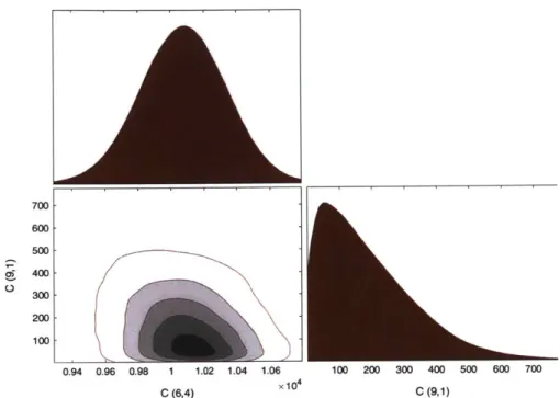
2-9 (6,4) and (9,1) pure component spectra. . . . . 73

2-10 Simulated measured data for an even mixture of (6,4) and (9,1) SWNTs

with normally distributed noise. . . . . 73

2-11 Posterior distribution of estimated SWNT concentrations in the two component example . . . .

. 74

2-12 Prior distribution assumed for MCMC sampling. . . . . 75

2-13 Posterior distribution of 6 parameters. . . . . 75

2-14 The posterior distribution (histogram) is much narrower than the prior

distribution for the center of the Ell transition for the (6,4) species. . 76

2-15 El center (6,4) nanotube marginal posterior distribution from MCMC

(bars) and linearized estimate from optimization (line). . . . . 76

2-16 Simulated measured data for an even mixture of (6,4) and (9,1) SWNTs

when nearly no (9,1) nanotubes are present in the mixture . . . . 77

2-17 Posterior distribution of concentration estimates for two species with

uncertain pure component spectral parameters when one species is near

2-18 Independent vs simultaneous analysis with five samples. Circles show

the median and 95% range of the posterior. The line and

+

show the true value. a) concentration of (6,4) species when estimated independently. b) concentration of (6,4) tubes when estimated simulta-neously c) independent estimation of Ell peak center d) simultaneous

estim ation E l . . . . 80

2-19 Upper Right Panel: Concentration estimates shared between 7

sam-ples. Lower Right Panel: Concentration estimates for 7 samples each

taken independently. Upper Left Panel: The simulated UV-vis-NIR

spectra for each of 7 samples. Lower Left Panel: The true

concentra-tion of each species in the simulated spectra. . . . . 81

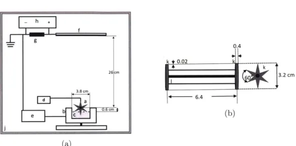
3-1 (a) Schematic of the apparatus for free surface electrospinning from

wire electrode on star-shaped spindles. The components are: (a) wire electrode, (b) solution bath, (c) solution, (d) DC motor, (e) high volt-age power supply, (f) collector plate, (g) 1 MQ resistor, (h) multimeter,

(j)

Schematic of the wire electrode with spoked wheels (k) and threaded rod (1) containing only two wires; (i) side view, perpendicular to spindle

axis, (ii) end-on view, parallel to spindle axis. . . . . 88

3-2 Formation of satellite droplets of aqueous solution of PVA (7 wt%) on

the wire, midway between mother droplets. . . . . 90

3-3 a) The average single jet behavior observed by Forward et al., under

different conditions of the PVP system b) The whole wire current ob-served as a sum of multiple overlapping individual jetting events c) The density of jets per length of wire estimated by Forward et al.'s

3-4 Example of current signal collected when multiple droplets are jetting (at 2.5 rpm and 45 kV). The current vs time contributions from indi-vidual jets at the onset of jetting clearly have a different shape than those of jets occurring later. The inset shows the average signal from

a single jet under the same processing conditions. . . . . 94

3-5 The piecewise linear parameterization for the current contribution of

a single droplet jetting from the wire electrode to the collection plate. This parameterization can provide an approximate description of the true single jet profiles shown in inset of Figure 3-4, with the exception of the final "tail". It is sufficiently flexible to model both the apparent jet contributions of "early" and "late" jets observed in Figure 3-4. . . . 95

3-6 Electric field strength near the surface of the wire electrode during

rotation . . . . 101

3-7 Liquid entrainment of 7 wt% aqueous PVA (146-186 kDa) solution.

Black dotted line is the power law fit to the data. . . . . 102

3-8 The correlation between wavelength parameter, 27rao/A , and applied

electric potential at a constant spindle rotation rate of 2.5 rpm. . . . 103

3-9 Current drawn from 7wt% PVA/water solution at 45 kV under different

spindle rotation rates of 2.5 rpm (black), 3.2 rpm (red), 5.6 rpm (green),

7.2 rpm (blue) and 8.7 rpm (magenta) as a function of angular wire

position. The differences in electric current profiles are indicatively of the variation in jetting with spindle rotation rate. (b) Angular range of jetting vs. rotation rate of spindle for an applied voltage of 45 kV.

3-10 Average current drawn from a single droplet at 45 kV at rotation rates

of 3.2 rpm (dashed), 5.6 rpm (dash dotted), and 8.7 rpm (solid). Error

bars correspond to one standard deviation determined from averaging over at least 10 current measurements for single jets. In the inset, the current profile is shown for a single jet that was allowed to jet only after the wire electrode crosses the apex of the arc of rotation (i.e., in

between 900 and 2030). . . . . 106

3-11 Optimal model fit to the wire current generated by the Bayesian model,

based on piecewise linearity of single jet profiles. The black solid line is the wire current data collected during a free surface electrospinning experiment by rotating the wire spindle at 5.6 rpm with Vappi = 45

kV. The heavy solid line that overlaps the data is the best fit obtained

from model. The thin solid lines in the figure represent different single jets as they appear at different angular positions in order to generate

the total current from the wire. . . . . 108

3-12 (a) The linear density of jets as a function of angular position and (b) electric field at different rotation rates: 3.2 rpm (dashed), 5.6 rpm

(dash-dotted), and 8.7 rpm (solid line) . . . . 109

3-13 (a) mean and standard deviation number of jets in contact at 2.5V

motor speed (b) mean and standard deviation number of jets in contact

at 3V m otor speed. . . . . 110

3-14 (a) sample total charge transfered for single jetting phenomena at 1.2V motor voltage, (b) empirical cumulative distribution of total charge transferred by single jets at the 1.2V motor voltage. . . . .111

3-15 Optimal model fit to the wire current generated by the piece wise

linear model with 4,5,6, and 7 total jets to the same total current. The blue solid line is the wire current data collected during a free surface electrospinning experiment by rotating the wire spindle at with 3V to the motor with Vappi = 45 kV. The green and red lines are best fits. The green fit is unconstrained piece wise profiles. The red line shows

constrained profiles by the prior knowledge of jet durations. . . . . .111

3-16 Model fitting to the experimental productivity data. Experimentally

observed productivity (filled symbols) at different rpms at applied po-tentials of 40 kV (square), 42.5 kV (circle), 45 kV (triangle), and 50kV (diamond). The entrainment-limited productivity as calculated from Equation 3.20 is shown by the solid line and the field-limited produc-tivities at different applied potentials as functions of rotation rate are shown by dashed lines. The transition from the entrainment-limited regime to the field-limited regime is most apparent in the data at 45 kV. 114

4-1 A diagram of sensor locations on a dual completion oil well. BHP:

Bottom hole pressure. BHT: Bottom Hole Temperature. WHP: Well Head Pressure. WHT: Well Head Temperature. ACCI, ACC2:

Acous-tic Sensors . . . . 121

4-2 Empirical cumulative distribution for bottom hole pressures and well

head pressure during bean ups or main production modes. . . . . 122

4-3 Well routing history for the well under study. The well state changes many times over the course of a wells operation between the

pre-identified labeled states associated with valve routings. . . . . 131

4-4 Parzen density estimator showing decision boundary tuned to reject

3% of data as outlying. The feature space axis are the first 2 principal

4-5 Left: Average weekly power demand in dutch power demand dataset, Right: outlying weeks found by feature space transformation (offset).

Time is in 15 minute increments. . . . . 136

4-6 Sample data from the Ford classification challenge dataset showing time series measurements from an engine subsystem. a) nominal

mea-surements b) anomalous behavior . . . . 138

4-7 Two classes of engine data shown projected down to two principal

components using 6093 features. . . . . 139

4-8 Distribution of classification performance of individual features with a

linear decision boundary. . . . . 139

4-9 Two classes of engine data shown in two highly separating feature

di-m ensions. . . . . 140

4-10 Scree plot showing the variance explained by each principal component of the ford data with 6093 features the red var shows the sum of the

rest of the principal components after the 30th component. . . . . 141

4-11 Scree plot showing the variance explained by each sparse principal com-ponent of the ford data with 6093 features. The SPCA was constrained

to have a specified number of features in each principal component. . 142

4-12 Two classes of engine data shown in two sparse principal component

with 6 features per sparse principal component. . . . . 143

4-13 The linear classification performance when trained on all 806 examples considered in the Ford dataset using SLDA with a specified number of features mapped as a linear combination to form a discriminating

direction. SLDA was trained with 12 penalty of le-6. . . . . 144

4-14 Distribution of measurement responses in dual completion low pressure

configuration. . . . . 145

4-15 Correlation of 6 main measurements in dual completion low pressure

state... ... 146

4-17 Bottom hole pressure portions of operating history colored time in the well's life from blue to green to yellow to red to dark red. The diamond points are shortly after restarts, the + symbols are near failure data

points and the open circles are putatively normal conditions. . . . . . 148

4-18 Acoustic detector 1 portions of operating history colored time in the well's life from blue to green to yellow to red to dark red. The diamond points are shortly after restarts, the

+

4-19 Three class classification performance trained with sparse linear dis-criminant analysis: a) acoustic detector 1, b) acoustic detector 2, c) bottom hole pressure, d) bottom hole temperature, e) well head pres-sure, f) well head temperature. . . . . 150

4-20 Three class classification performance trained with Sparse Linear Dis-criminant Analysis with merged HCTSA features in acoustic 1 and 2, bottom hole temperature and pressure, and well head pressure. . . . . 151

4-21 Scatter plot of the well 1 data projected into SLDA directions with a sparsity level of 40 features per direction. . . . . 152

4-22 Boundaries for anomaly detection trained to reject 3% of putatively nominal data. Data was the first two principal components projected from HCTSA features. a) acoustic detector 1, b) acoustic detector 2, c) bottom hole pressure, d) bottom hole temperature, e) well head pressure, f) well head temperature. . . . . 157

4-23 Number of dimensions each in which each day long portion of operating history was found to be anomalous at a 3% outlier selection rate by a Parzen density estimator in two principal component reduction of a HCTSA feature space. . . . . 158

4-24 Anomalous behavior identified on March 4th. . . . . 158

4-25 Anomalous behavior identified on March 6th. . . . . 159

4-27 Boundaries for anomaly detection trained to reject 3% of putatively nominal data with a Parzen density estimator. a) Data was the first two principal components projected from HCTSA features for 5 mea-surements (not using WHT). b) Data was the two disciminatory direc-tions found via SLDA with a sparsity level of 40 components projected

from HCTSA features for 5 measurements (not using WHT). . . . . . 160

Al SVD spectra with discretization . . . . 163

B1 Empirical cumulative distribution function of the wht showing gaps in the data... ... .... .166

B2 Evaluation of the optimal number of clusters using the Calinski-Harabasz clustering evaluation criterion. Higher is better. . . . . 166

B3 Evaluation of the optimal number of clusters using the Davies-Bouldin clustering evaluation criterion. Lower is better. . . . . 167

B4 Distribution of data points in cluster 1 of 4 found by kmeans for LPLP data. ... ... 167

B5 Distribution of data points in cluster 2 of 4 found by kmeans for LPLP data. ... ... 168

B6 Distribution of data points in cluster 3 of 4 found by kmeans for LPLP data. . ... ... .. ... ... .. .. 169

B7 Distribution of data points in cluster 4 of 4 found by kmeans for LPLP data. ... ... 170

B8 Four clusters identified by color in the LPLP data . . . . 171

B9 Static data colored by time point . . . . 172

List of Tables

2.1 Transition Energies for (15,2) and (16,0) SWNTs . . . . 55

2.2 Comparison of regularization strategies at recovering true concentra-tions of mixtures of nanotubes in the correctly specified pure compo-nent spectra setting with various regularization strategies, noise levels

and sparsity of underlying signals. . . . . 62

2.3 Minimum Diagonal Element of Model Resolution Matrix . . . . 66

2.4 Error from using overly simplified pure component models . . . . 66

2.5 Parameters in a spectral model including peak centers, side peaks, peak

widths, peak shape and relative oscillator strength. . . . . 68

3.1 Comparison of solution properties of 7 wt% PVA/water (this work)

and 30 wt% PVP/ethanol [40] . . . . 88

3.2 Bayesian Optimization Prior Parameters and Model Parameter . . . . 99

4.1 Multivariate Data Organization . . . . 132

4.2 Number of statistical significant bilinear and quadratic second order

terms at the p < 0.001 level . . . . 143

A. 1 The properties of 43 semiconducting nanotube species that were used

Chapter 1

Introduction

Rapid increases in instrumentation and computation have presented an increase in data collection capabilities in many industrial and scientific systems. Traditional paradigms of engineering have often been centered around first principles or semi-empirical mathematical modeling techniques. In this thesis an alternative scientific paradigm of working first from data, rather than predominantly relying on estab-lished theory is explored. Of course, most theories are developed from extended observations and controlled experimentation which naturally involve the collecting and understanding of data. However, in complex systems, the data can often be ex-ploited without relying upon building detailed models from established theory for all parts of the system.

The applications of statistical modeling and learning contained in this thesis en-compass three applications to chemical engineering problems which span a range of relative importance of data versus existing detailed theory. These projects introduce a broad conceptual tool which is understanding the gradient of available theory and ex-isting models versus the quality of data available to understand the system. The first project involves the utilization of a detailed physical model, and small data. The use of the model for parameter estimation is evaluated with computational Bayesian meth-ods allowing for the quantification of uncertainty in estimates. The second project involves as system where the complexities of the dynamic physical process are such that the direct application of a detailed physical model was not viable. In this project

an empirical model was derived to be sufficiently flexible to approximately model the dynamics of the system, and the results of the analysis made subsequent analysis of the experimental system possible. The final problem tackled relied on using data directly via the transformation of dynamic time series data to a high dimensional static feature space to build a probabilistic model for anomaly identification so that deviations from nominal behavior could be identified.

The common link between the projects in this thesis is the role of tools from com-putational statistics and machine learning in problems from chemical engineering. This chapter provides a brief background on computational Bayesian inference, prob-abilistic modeling, uncertainty quantification and anomaly detection and diagnosis necessary for the applications described in subsequent chapters.

Chapter two describes work on statistical estimation with a detailed physical model combined with softer assumptions. The application motivating the work is the quantification of uncertainty associated with estimating the relative abundance of mixtures of carbon nanotubes in aqueous solution.

Chapter three describes work on deconvolution of electrical signals generated from a free surface electro-spinning apparatus. In this application a detailed parametric model of the physical system with all uncertain parameters was not available so only an approximate model of the system was utilized. This chapter describes the experimental data collected, approximate model construction and utilization of the results of the approximate model in subsequent analysis.

Chapter four describes work utilizing a data driven approach for oil well monitor-ing. This work introduces a transformation of time series data into a feature space description. Discriminative techniques were utilized to analyze the data collected from the well.

1.1

Historical Perspectives and Motivations for

Com-putational Statistics and Data Science

In conducting scientific and engineering work, a term has recently been an introduced to describe a trending epoch towards data intensive science, this is called the fourth paradigm [82]. In this breakdown of the history of science, the first paradigm is em-pirical, where it consisted of describing natural phenomena. The second paradigm has been a more recent development of theoretical methods, using mathematical mod-els and generalizations. With the advent of computing machines, a third paradigm of science related to simulation has emerged. The fourth paradigm is again a com-putational revolution, but seeks to unify theory, experiment and simulation. Data captured by instruments or generated by simulations has to be processed by compu-tational work-flows before information, knowledge and insights can be generated. This scientific inquiry through data processing is at the heart of many recent revolutions in genetics, and the other -ohmics of bioinformatics.

At the same time as this revolution in scientific process has been possible, a mas-sive increase in computational capacity and data acquisition has evolved. For the last several decades the computational performance of CPU chips has rapidly increased following the miniaturization of transistors (Moore's Law). Problems with waste heat and fundamental physical limits have presented issues with per CPU performance gains with time. However, multiple strategies for parallelization have gained main-stream acceptance allowing for greater computational efficiency per watt or per dollar. The first is multi-core CPUs. The second is general purpose computing on graphical processor units which allows for very efficient parallelized operations of some com-putations. Additional parallelism exists in cluster computing infrastructures which exist in both high performance computing infrastructures and commodity cloud based systems. Most recently strongly enhanced performance for distributed computation on large data sets has become possible with increased use of in memory data storage.

By leveraging these foundational increases in computation and data storage

Cloud based Internet service providers such as Amazon Web Services, or Microsoft Azure offer machine learning pipelines as flexible and scalable services.

1.1.1

Industrial Data Science

With the rise of intense instrumentation and data recording capacities in industrial and computational systems, there has become a very large number of variables for system operators or process operators to monitor during chemicals manufacturing or other industrial tasks. Effectively monitoring these large complex systems is expected to increase in difficulty because the volume of data is so large and growing. Industrial systems such as chemical plants may have tens of thousands of variables which are measured continuously. Large server farms and cloud systems can similarly have a large number of hardware and software defined variables being tracked continuously. Critically, the data are multivariate and have correlations or are otherwise in-terrelated and the maximum value of analyzing the data can only be accessed by simultaneous evaluation. To assist human operators in assimilating the volume of data available, the development of automatic data analysis systems has been an on-going area of interest.

An example of the cross over of domains between industrial and "tech" systems is readily apparently in anomaly detection and diagnosis. The consumer web companies Twitter and Netflix released anomaly detection software packages for monitoring their

server hardware and software processes.1 Both of these packages are designed for

univariate analysis for a one dimensional time series of floating point values at a time. These packages are developed to account for critical factors of seasonality and periodicity in measurements due to changing human behavior with time of year, day of week and hour of day. In contrast in the engineering and industrial statistical process control literature, methods for handling multivariate methods are quite mature and most processes are designed with hierarchical control systems such that the process can be maintained in a steady state damping daily or weekly variability. In the engineering and industrial statistics literature multivariate control charts are a well

studied example of using multiple measurements simultaneously and gaining value from the correlation in multiple measurements.

Practitioners in a multiplicity of different domains are recognizing the value of data collected during normal business of scientific processes and the opportunities present, and organizing to work in a data driven fashion. One emerging challenge in generating value from data, is surfacing the data from databases or other systems designed to store historical data and supporting real time actions and decision making. Moving computational systems into real time applications requires engineering of not only the algorithms and statistical methods being applied but also the computational work flow and data handling processes. This promotes a synergistic relationship between expertise in data management and storage, software, machine learning methods and engineers and scientists.

With a sufficient degree of abstraction a lot of the challenges faced by a network operations engineer, or a site reliability engineering are very similar to those faced by someone monitoring and administering an industrial process. However, there exists a gap in familiarity with the specifics of the problems faced in each domain. This presents an ample opportunity to cross fertilize ideas from multiple previously isolated communities.

It is unlikely the industrial, manufacturing, or chemical engineers will know about columnar data stores, and distributed in memory computation, but traditional big data engineers will have a hard time selling to the chemical manufacturing industry because they don't understand the problems, and don't understand the kinds of data acquisition and control systems technologies that are already embedded.

In the final chapter of this thesis the understanding of an oil well system is gen-erated predominantly from a data mining exercise. This bottom up approach of understanding engineered systems based on the data is made more powerful from the availability of low-cost computation and storage, the advancement in computational statistical methodologies, and the improvement in engineering understanding of how to handle data among the workforce.

1.2

Probabilistic Modeling and Machine Learning

The field of machine learning can be considered as a large and evolving set of methods for detecting relationships in datasets and predicting future relationships. The notions of probability provide a natural framework for understanding the relationships in data, uncertainty in data, and making predictions. Probabilistic modeling is used throughout this thesis to ensure robust and sensible procedures to map from data to actions or insights.

The work in this thesis involves both halves of the classic paradigm split of su-pervised and unsusu-pervised learning. Susu-pervised learning involves learning a mapping from input data to output labels, whereas unsupervised learning is focused on learning interesting patterns or relationships in data and not a specific predictive relationship. The work in Chapters 2 and 3 is formulated a regression problem, while Chapter 4 is focused on unsupervised learning and a one-class classification problem.

Often when tasked with the problem of interpreting some data the most conven-tional practice is to draw a line through the data, report the slope and intercept and move on. The most common form of fitting this line to the data is done via minimiza-tion of the least squares error of the line and the data. The least squares strategy represents a selection of a particular loss function to be minimized to select some parameters for the model. This selection of an objective function for minimization introduces assumptions about the underlying statistical behavior of the dataset that are often incorrect in practice. The selection of a least squares objective function is often done out of force of habit and lack of sophistication on the part of the analyst. There are many possible alternative choices for an objective function.

By introducing a generative model for the data, interpretable probabilistic

infer-ence is possible with, the assumptions of the model and analysis strategy being clearly specified and interpretable. A generative model is a mathematical expression or com-putation procedure that is parameterized to quantitatively describe the procedure

that could have reasonably generated the data

[46].

Subsequently, the particular form of the objective function to be minimized to find a point estimate of the parameters can be often found explicitly and analytically as function of the data in simple problems, or as a relatively simple computational expression in cases where an analytic solution is not possible.

By working in the framework of probabilities, computational strategies or

applica-tion logic such as rules for anomaly detecapplica-tion can be found from a firmer foundaapplica-tion than simply proscribing them based on the analysts whim and some validation that they work in some cases.

1.2.1

Constructing a Model

When constructing a probabilistic model for a system or dataset a valuable tool is

consider the representation of a graphical model. See [66] and

[65]

discussion.

The benefits of constructing a generative model which relates quantities of interest to data are numerous. Upon constructing a probabilistic interpretation of data even if only approximate, the subsequent analysis procedures have arbitrariness removed and assumptions more directly composed.

One way to build a probabilistic model is to create a joint model of the data and parameters of interest p(y, x) where y is the data and x the parameters of interest and then to condition on x, thereby deriving p(ylx). This is called the generative approach [66].

The generative model framework is contrary to discriminative modeling. The difference between these approaches is perhaps best understood in the context of classification. In classification discriminative approaches seek to maximize an ob-jective by specifying some form of boundary between classes whereas in generative approaches the joint distribution of class labels and input values is learned from data. Generative models have strengths and weaknesses relative to discriminative approaches. In particular the discriminative approach may be less sensitive to model data mismatch because it doesn't need to learn an entire distribution but rather in classification tends to be concerned with only the class boundary. Generative models

have the advantage of being symmetric in inputs and outputs and can be utilized for a variety of analytical tasks such as predicting the distribution of outputs given inputs. This is key for the working in Chapter on parametric modeling of optical spectra of mixture of carbon nanotubes. In Chapter 4 working on the feature space transformation of data the statistical assumptions about different features are harder to encode correctly when formulating a model.

1.2.2

Regression Models

The formulation of regression models with additive noise models application to simu-lated and experimental data is the central subject of Chapter 2 and Chapter 3. The formulation of regression models here follows the probabilistic interpretation of linear regression.

It is well known that the conventional weighted least squares is the maximum like-lihood estimator and minimum variance unbiased estimator when a set of N points (xi, yi) is available with perfect knowledge in the x coordinate and Gaussian uncer-tainties with known variance o. for each measurement. Positing a linear relationship between the x and y data gives a model for the y values as a function of x as in Equation 1.1.

f (x) = mx+ b (I.)

The objective of the analyst is to then find the quantities m and b such that a best fit is observed. The linear algebra solution to the such a circumstance is to stack

up the data, indexed by i, into the form y = AO, 6 = [b, m]T, Ai,: = [1, xi], yi = yi.

The uncertainties in y then get introduced into a covariance matrix C,i of., C. , =

Ot j.

0= = [AT C A] 1 _[ATC-y]

(1.2)

scaled total squared error between the right and left hand sides of y = AO. This makes this particular selection of parameters the best fit under a context where this scaled error is the error an analyst desires to minimize. The justification as a mini-mum variance estimator and maximini-mum likelihood estimator requires a more detailed probabilistic description. The choice of the model and choice of objective function are the problems that must be fully justified in analysis. The choice of how to find optimal value of a scalar objective function can then be addressed via engineering expediency considerations.

Production of a generative model for the data and evaluating the posterior distri-bution of the unknown parameters is the most sensible and justifiable approach for analysis of regression problems. The generative model introduced in Equation 1.1 is that the process which generates the data is described by the conditional probability distribution for observations yi, given everything else in Equation 1.3.

( 2 b) 1 exp(- (yi - mxi - b)2 (13)

p~~y07l97,

oYm )=

13

The transformation of this generative model to a scalar objective to be optimized, found explicitly deciding to determine the point estimate of the parameters that maximize the probability of the data we observed. This is the maximum likelihood estimate of the parameters. Because in this simple formulation the data is inde-pendent when conditioned on the particular value of the parameters the total data observation probability is a product of the condition probabilities of each observation. This joint probability is called the total likelihood function L in Equation 1.4.

N

1 f P(yiIXi, of., m, b) (1.4)

i=1

objective function which can be maximized using blackbox optimization procedures. However, taking the log transformation of Equation 1.4 gives the log-likelihood which

is a more convenient function to optimize which is within constant factors of x2 which

gives that minimization of the X2 error is the maximum likelihood estimator because

the log transformation and dropping of scalar factors do not change the optimal parameter values found in optimization.

An alternative selection of estimators is to use Bayes' theorem and derive the posterior distribution of the unknown parameters given the data and uncertainty. The posterior distribution for this two parameter linear model is given in Equation

1.5.

(My0, xi, u2 Vi)p(0 1xi, o2Vi)

p(o|yi, Xi, a Vi) = P( YiY (1.5)

p(yi Xi, o-2Vi)

In Equation 1.5 the posterior distribution is found via Bayes' theorem first creating the joint distribution of the uncertain observations y and unknown parameters 0 as the product of the likelihood and the prior distribution of the parameters in the numerator and then conditioning on the data yi, where everything is conditioned on the data considered to be known exactly (- and x).

Finding a point estimate from a posterior distribution can be done in a number of ways the simplest of which is to maximize this posterior distribution and find the MAP or maximum a posteriori value of the uncertain parameters. For uninformative selections of prior distributions this corresponds precisely with the maximum likeli-hood estimates. In some cases the posterior distribution may be analytically tractable to calculate and the entire distribution can be found often as a parametric expres-sion of a few parameters, or the first several moments of the distribution calculated explicitly. In Chapter 2 for sufficiently complicated problems we find this to not be possible and resort to Markov Chain Monte Carlo methods to approximately sample from the posterior distribution and then construct the estimate of the mean from these samples.

for purposes of regularizing point estimates. In this discussion and estimator is a procedure which maps from data to a point estimate of parameters of interest. The bias of an estimator (Equation 1.6) is the expected value of the deviation from the true value of parameters observed by an estimator. The point estimate of parameters is called 0 while the true value is 0*. This expected value is taken over the true distribution of parameters p(Q*) which is the frequency distribution of true values we could ever expect to observe in our experiment.

Bias(0) = E(*)(o - 0*) (1.6)

The variance of an estimator is an idea of the precision of an estimator or its sensitivity to the noise or inherent stochasticity of an estimation problem.

Variance(6) = Ep(o*)(6 - E(6))2 _(1.7)

1.3

Uncertainty Quantification and Propagation

In the analysis of standard linear least squares problems as discussed in Chapter 2, the uncertainty in estimated parameters 0 can be evaluated analytically provided the assumptions of the model are assumed to hold exactly. The resulting uncertainty around the point estimate in parameters is multivariate Gaussian with 0 mean and covariance matrix:

0

1mbT

cov(0) - b om,b - [AT C-A]-1 (1.8)

L m,b am J

This description of the uncertainty in the estimated parameters is of course de-pendent on all of the assumptions holding exactly. When the posterior distribution of parameters is constructed then the uncertainty description is naturally described not in terms of an expected distribution of a point estimate, but rather as a "credible" in-terval for parameters combinations of parameters. Such inin-tervals can be constructed analytically under some circumstances, but are more generally evaluated from draw-ing samples from a posterior distribution. This is the approach taken in Chapters 2

and 3 for evaluating uncertainty in complex models. Bayesian methods importantly offer the ability to evaluate the marginal uncertainty in some parameters account-ing for the fact that their may be unknown but uninterestaccount-ing parameters in many applications.

Uncertainty in estimates can be evaluated can also be evaluated non-parametrically

by re-sampling methods such as the bootstrap or jackknife.

1.4

Anomaly Detection and Diagnosis

From a probabilistic perspective in this thesis anomaly detection and diagnosis is viewed as examining the posterior probability that a given input is anomalously dif-ferent from nominal behavior. The input may be a scalar or vector input or as will be discussed in Chapter 5 sequence of observations. Anomaly detection has often been considered in the context of classification problems between two or more classes. Often this work is introduced under the paradigm of fault detection because the types of faults are assumed to be known in advance and in this context sufficient data is available about the distribution of data under faulty conditions. In this case the clas-sification performance on training and test data is the core metric for evaluating the success of the methods under study or development.

An alternative related problem is that of novelty detection where data is avail-able exclusively under known nominal conditions where the data is all labeled with one class in the training context with none of the training examples expected to be anomalous.

In the outlier detection problem context the available data is assumed to be largely in one class (nominal) but some fraction of the data which may be known or unknown should be properly identified as an anomaly. This context is especially difficult if the fraction of training data which contains outliers is unknown. This is principally the context of the oil well ADD problem. In this case without labeled data the success of the method is reliant of ex post facto investigation of the points or portions of operating history identified as outliers and inliers and the distributional or statistically

properties of the decision boundaries and datasets produced.

In the classification context, two perspectives on the problem exist a geometric or discriminative perspective and a generative or probabilistic perspective. In the generative perspective the classes belong to separate probability distributions, and the determination of which class a new example belongs to is given by the Bayes decision rule given in Equation 1.9 assuming an equal preference for misclassification.

For two classes C1, and C2 a new observation x is assigned such that it is in the class

for which it has maximum a posteriori probability:

x E C, C, = argmax (P(C Ix)) (1.9)

CiG[C1,C2]

The posterior probability P(Cilx) is found via Bayes rule which is given in Equa-tion 1.10. The posterior probability joint probability of class assignment and obser-vation conditioned on the marginal probability of the obserobser-vation.

P(Ci X) = P(X Ci)P(Ci) (1.10)

P(x)

The joint probability of class assignment and observations is factored into two terms P(Ci) called the prior probability of a class and P(xlCi) which is the likelihood for observations conditioned on being in a particular class. This is a generative prob-abilistic model which describes the probability of observations in fault and non-fault states. The specification of this model is at the heart of many generative classification problems. The identification, assumption or learning of a particular distributional re-lationship for the data is what drives the differences between generative classification methods. For example assuming that observations are multivariate normally dis-tributed with different means and covariance structure in each class, and identifying these distributional parameters with maximum likelihood estimation is referred to as quadratic discriminant analysis (QDA) as the decision boundary is found as a quadratic function between the two classes. If shared covariances are assumed in

such a mixture of Gaussians model results in linear discriminant analysis (LDA) with a linear decision boundary between each class [66].

Chapter 2

Uncertainty Analysis in Spectroscopic

Chemometrics: Regularization,

Sequential Analysis, and Bayesian

Estimation with a Detailed Model

2.1

Introduction

This chapter addresses the problem of estimating the concentration or relative abun-dance of a mixture of species of single-walled carbon nanotubes in solution. Analogous problems regularly occur in quantitative chemical analysis. The details of the prob-lem as applied to carbon nanotubes allow for comparison of existing classical methods and more advanced optimization based analyses. To address the question of evalu-ating the uncertainty in analysis we resort to computational Bayesian inference with a hierarchical probabilistic model including prior distributions for uncertain spectral lineshape parameters. Strategies for rejecting noise and improving the quality of in-ference are reported for classical methods, optimization methods and in cases with sequential measurement data.

measurement of single walled carbon nanotubes and why that gives rise to particular forms of uncertainty. Next estimation of relative abundance with noisy data under various modeling assumptions in linear models is reviewed. The impact of regulariza-tion strategies such as Tikhonov regularizaregulariza-tion and the Lasso method, for improving concentration estimates from chemometric models for concentration estimation from absorbance or photoluminescence excitation spectroscopy is demonstrated. The qual-ity of performance of these methods is demonstrated in numerical simulation studies. The uncertainty and confidence intervals on from analysis using these procedures is introduced. Improvements in analysis in this simpler context for sequential data is presented. An increase in complexity of analysis for systems with incorrect model specification is subsequently introduced. This necessitates the introduction of a non-linear parametric model for the uncertainty in lineshape. The impact on the analysis with linear estimation strategies with model misspecification is examined theoreti-cally and with computational examples. Regularization and sequential data analysis strategies are shown to reduce the impact of model misspecification for certain error metrics. Finally the complete set of parametric uncertainty in the model is evaluated with a hierarchical probabilistic model and compared to simpler analysis strategies.

Reduction in uncertainty in estimates is improved in contexts where multiple measurements of the same or related populations of species in solution are available. Improvements for sequential data analysis are demonstrated as a reduction in error from true concentration profiles in hypothetical separation experiments.

2.2

Notation

In this chapter vector quantities are represented as bold lower case symbols such as

O or d. Matrix quantities are given as bold uppercase characters such as A. Normal

weighted symbols will be used for scalar quantities. Subscripts will be used to indicate elements of vectors, or matrices. The notation Ai,: will indicate the entire i-th row of

2.3

Background

2.3.1

Carbon Nanotubes

Single-walled carbon nanotubes (SWNTs) are a class nanomaterials that consist of

a cylindrical arrangement of pure carbon atoms which are covalently linked by sp2

bonds. The arrangement of these atoms can be considered as that of a sheet of graphene, which has been rolled up with a particular angle relative to the hexagonal structural unit cell of 2-d carbon. These materials are interesting to researchers in a wide variety of areas. In particular these materials have interesting mechanical, electronic, and thermal properties. SWNTs like many nanomaterials, exhibit hetero-geneity in atomic structure. SWNTs can vary in a number of partially independent attributes such as the relative orientation of the tube axis to the carbon unit cell, the diameter of the tube, and the length of the tube. For the purposes of this work, SWNTs are considered with small diameters from 0-10nm and short lengths from hundreds of nanometers to a few micrometers. Though greater variation in length and diameter is possible, especially if the subject of interest is broadened to include multi-walled nanotubes rather than only single-walled carbon nanotubes. The

diame-ters and roll up angles uniquely correspond to set of chiral indices (n, m) which index

all possible roll-up angles and diameters. The chirality of SWNTs strongly impacts the electronic structure. The chiral indices can be used to approximately understand the electronic behavior. SWNTs with n-m mod 3 = 0 are metallic or semi-metallic and the rest are semiconducting. The electronic structure of SWNTs is complex. The best available data on the primary electronic transitions of semiconducting nanotubes is available in Liu et al., 2012 [58]. The variation of properties is of significant scien-tific and commercial interest as people endeavor to build sensitive chemical sensors or chemical components out of these materials. A major obstacle in the study of SWNTs and in the deployment of SWNTs in scientific and industrial applications has been that the conventional methods of synthesis such as arc discharge, laser ablation, and chemical vapor deposition, produce populations of CNTs that are not uniform [45]. As-synthesized nanotubes exhibit a distribution of lengths and chiralities as well as

impurities. Because of this variation, the purification and characterization of SWNTs is an important step in device development.

Great progress has occurred in recent years in characterizing populations of single walled carbon nanotubes (SWNTs) in solution through optical spectroscopy [76, 85, 4]. This progress has been developed in parallel to techniques focused on the separation of carbon nanotubes and isolating them in solution. These techniques have resulted in the ability to approximately uniquely identify different species of SWNTs by

elec-tronic bandgap by photoluminescence (PL) (excitation) spectroscopy

[4].

of uniformity in the properties of as-prepared SWNTs motivated significant efforts in the development of techniques to sort and separate populations of SWNTs. Separa-tion methods have been simultaneously advanced with methods designed to support the selective growth and synthesis of SWNT populations. Current techniques in se-lective growth have not been fruitful enough to eliminate the need for sorting and separation. Techniques have been developed to sort and separate SWNTs based on diameter/ chirality, length, and metallic/ semiconductor character.

One of the earliest developed approaches for the separation of SWNTs by chirality and therefore electrical properties is by density gradient ultracentrifugation (DGU).

DGU has been developed as a suitable technique for sorting by diameter, electronic

properties, and of most interest to this work: specific chirality and helicity [45, 2, 94, 10, 33, 42, 96]. DGU operates by separating different types of SWNTs that have been wrapped in surfactant molecules on the basis of differing buoyant densities. The technique utilizes a density medium to establish a gradient of density with position in a centrifuge tube. Various combinations of surfactants can be used to establish the differences in buoyant density among nanotube species, based upon the electronic interactions between the surfactants and the nanotube. Common surfactants include short segments of DNA (ssDNA), sodium deoxycholate (SDC) and sodium dodecyl sulphate (SDS) among others.

In addition to DGU another promising technique for separations is gel chromatog-raphy [57]. This method exploits the structure-dependent strength of interaction of the SWNTs with an allyl dextran-based gel matrix in a series of vertically connected