Surface Reconstruction from Multi-View Stereo of Large-Scale Outdoor Scenes.

HAL Id: inria-00503837

https://hal.inria.fr/inria-00503837

Submitted on 21 Jul 2010

HAL is a multi-disciplinary open access

archive for the deposit and dissemination of

sci-entific research documents, whether they are

pub-lished or not. The documents may come from

teaching and research institutions in France or

abroad, or from public or private research centers.

L’archive ouverte pluridisciplinaire HAL, est

destinée au dépôt et à la diffusion de documents

scientifiques de niveau recherche, publiés ou non,

émanant des établissements d’enseignement et de

recherche français ou étrangers, des laboratoires

publics ou privés.

Nader Salman, Mariette Yvinec

To cite this version:

Nader Salman, Mariette Yvinec. Surface Reconstruction from Multi-View Stereo of Large-Scale

Out-door Scenes.. International Journal of Virtual Reality, IPI Press, 2010, The International Journal of

Virtual Reality, Volume 9 (Number 1), pp.19-26. �inria-00503837�

Abstract—This article describes an original method to reconstruct a 3D scene from a sequence of images. Our approach uses both the dense 3D point cloud extracted by multi-view stereovision and the calibrated images. It combines depth-maps construction in the image planes with surface reconstruction through restricted Delaunay triangulation. The method may handle very large scale outdoor scenes. Its accuracy has been tested on numerous outdoor scenes including the dense multi-view benchmark proposed by Strecha et al. Our results show that the proposed method compares favorably with the current state of the art.

Index Terms—Delaunay refinement, Multiple-views, Restricted Delaunay triangulation, Surface reconstruction.

I. INTRODUCTION

M

otivations. Various applications in Computer Vision, Computer Graphics and Computational Geometry require a surface reconstruction from a 3D point cloud extracted by stereovision from a sequence of overlapping images. These applications range from preservation of historical heritage to e-commerce through computer animation, movie production and virtual reality walkthroughs.

Early work on reconstruction has been focused on data acquired through laser devices, with characteristics that the obtained 3D point cloud is dense and well distributed [1]-[3]. Although these reconstruction methods have been reported as successful, the nature of the laser scanners greatly limits their usefulness for large-scale outdoor reconstructions. The recent advances in multi-view stereovision provide an exciting alternative for outdoor scenes reconstruction. However, the extracted 3D point clouds are entangled with redundancies, a large number of outliers and noise. Fortunately, on top of these point clouds, the additional information provided by the calibrated images can be exploited to help surface reconstruction.

Related Work. Over the past three decades there have been significant efforts in surface reconstruction from images, typically targeting urban environments or archaeological sites. According to a recent survey provided by Seitz et al. [4], the

Work partially supported by the ANR (Agence Nationale de la Recherche) under the “Gyroviz” project (No ANR-07-AM-013) http://www.gyroviz.org

Nader.Salman@sophia.inria.fr

surface reconstruction methods can be roughly categorized into 4 classes. The first class operates by computing a cost function on a 3D volume, which is later on used to extract a surface mesh from it. It includes the voxel colouring algorithms [5] and the graph cut algorithms [6]. The second class includes the variational methods and work by iteratively evolving a surface to minimize an error function [7]. The third class of methods is based on multiple depth-maps, ensuring a consistent 3D scene [8]-[13]. Finally, we call the fourth category of algorithms as hybrid algorithms. These algorithms mainly proceed in two phases: First, they extract a set of 3D points that are robustly matched across the images; second, they fit a surface to the reconstructed oriented 3D points [14, 15, 18, 19]. The recent work of Vu et al. [16] interestingly mixes a 3D volumetric method and implicit methods to output high quality meshed models.

Surface reconstruction from multiple views can also be thought in terms of the scenes they can handle. The requirements for the ability to handle large-scale scenes discards most of the multi-view stereo reconstruction algorithms including the algorithms listed in the Middlebury challenge [4]. The methods which have proved to be more adapted to large-scale outdoor scenes are the ones that compute and merge multiple depth-maps. However, in multiple situations, the reconstructed 3D models lack of accuracy or completeness due to the difficulty to take visibility into account consistently. Recently, two different accurate reconstruction algorithms have been proposed in [14], [16]. We demonstrate the efficiency of our reconstruction results relying on the publicly available quantitative challenge from the review of Strecha et al. [17] currently led by [14] and [16].

Contributions. Our reconstruction method is close to [18] and to the image-consistent triangulation concept proposed by Morris and Kanade [19]. It consists in a pipeline that handles large-scale scenes while providing control over the density of the output mesh. A triangular depth-map is built in each image plane, respecting the main contours of the image. The triangles of all the depth-maps are then lifted in 3D, forming a 3D triangle soup. The similarity of the triangle soup with the surface of the scene is further enforced by combining both visibility and photo-consistency constraints. Lastly, a surface mesh is generated from the triangle soup using Delaunay

Surface Reconstruction from Multi-View

Stereo of Large-Scale Outdoor Scenes

Nader Salman

1

and Mariette Yvinec

1 1 INRIA Sophia Antipolis, France1

Fig. 1. (a) the Voronoi diagram of a set of 2D points; (b) its dual Delaunay triangulation. (c) The Delaunay triangulation restricted to the blue planar closed curve is plotted in black. (d) The Delaunay triangulation restricted to the yellow region is composed of triangles whose circumcenters are inside the region.

refinement methods and the concept of restricted Delaunay triangulation. The output mesh can be refined until it meets some user-given size and quality criteria for the mesh facets. A preliminary version of this work appeared as a video in the ACM Symposium on Computational Geometry 2009 [20] and as a short paper in the Modeling-3D workshop of the Asian Conference of Computer Vision 2009 [21].

II. BASICNOTIONS

In this section we define the concepts borrowed from computational geometry that are required for our method. Let P = {p , … , p }_{0 n} be a set of points in Rdthat we call sites. The Voronoi cellV p )( _i , associated to a sitep_i, is the region of points that are closer top than to all other sites in_i P:



i j



d

i p R i j p p p p

p

V( )  :  ,   

The Voronoi diagram V(P)of P is a cell decomposition of d

R induced by the Voronoi cellsV (p_i).

The Delaunay complex D(P)of P is the dual of the Voronoi diagram, meaning the following. For each subsetI P , the convex hull conv( )I is a cell of D(P) iff the Voronoi cells of points in I have a non empty intersection. When the set Pis in general position, i.e. includes no subset of d 2 cospherical points, any cell in the Delaunay complex is a simplex. This Delaunay complex is then a triangulation, called the Delaunay triangulation. It decomposes the convex hull of P into

Let  be a subset ofR , we call Delaunay triangulation of

P restricted to  and we note D (_ P) , the sub-complex ofD(P), which consists of the faces of D(P)whose dual Voronoi faces intersect . This concept has been particularly fruitful in the field of surface reconstruction, where d 3 and

Pis a sampling of a surfaceS . Indeed, it has been proved that under some assumptions, and specially if P is a “sufficiently

dense” sample ofS , D (_S P)is homeomorph to the surface S and is a good approximation of S in the Hausdorff sense [22]. Fig. 1 illustrates the notion of restricted Delaunay triangulation.

The Delaunay refinement surface meshing algorithm builds incrementally a sampling Pon the surface S whose restricted triangulationD (_S P) is a good approximation of the surfaceS . At each iteration, the algorithm inserts a new point ofS into

Pand maintains the 3D Delaunay triangulation D(P)and its restrictionD (_S P) . Insertion of new vertices is guided by criteria on facets ofD (_S P):

 the angular bound controls the shape of the mesh facets;

 the distanced governs the approximation accuracy of the mesh elements;

 the size parameter l governs the maximal edge length of the mesh facets.

The algorithm [22] has the notable feature that the surface has to be known only through an oracle that, given a line segment, detects whether the segment intersects the surface and, if so, returns the intersection points.

At last, we also use the notion of 2D-constrained Delaunay triangulation based on a notion of visibility [23]. LetGbe the set of constraints forming a straight-line planar graph. Two pointspand q are said to be visible from each other if the interior of the segment pq does not meet any segment of G. The triangulation T in 2

R is a constrained Delaunay triangulation ofG, if each edge of T is either an edge of G or a constrained Delaunay edge. A constrained Delaunay edge is an edgeesuch that there exist a circle through the endpoints of e that encloses no vertices of T visible from an interior point ofe.

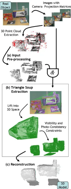
III. THERECONSTRUCTIONALGORITHM The algorithm takes as input a sequence of calibrated images and a set of tracks provided by multi-view stereo. The algorithm consists of three steps: 1) merging, filtering and smoothing the tracks, 2) building a triangle soup, and 3) computing from the triangle soup a mesh modelling the scene. The different steps of our algorithm are illustrated in Figure 2.

algorithm in more detail.

3.1 Merging, Filtering and Smoothing

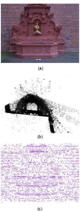
Figures 3a-3b shows the typical input to our surface reconstruction algorithm provided by a stereo vision algorithm. In this case the results were obtained from a set of 11 images taken from slightly different view points. Each input track stores its 3D point location as well as the list of camera locations from which it was observed during acquisition. In the following, we call line-of-sight the segment from a camera location to the 3D position of a track seen by this camera. Despite the robust matching process used by the multi-view stereo algorithm, the extracted tracks require some pre-processing [24] including merging, filtering and smoothing.

Merging. The first pre-processing step in our method consists in merging tracks whose positions are too close. We do that by building an incremental Delaunay triangulation of the 3D positions of the tracks. Each time a track 3D position is to be added, its nearest neighbour is requested, depending on the distance between these two track 3D positions one of two cases can arise.

If the nearest neighbour is close, with respect to a threshold₁, the two tracks are merged in a single one and their list of cameras is updated to include the union of the cameras of the two merged tracks. If the closest neighbour is at a distance larger than₁then both tracks are preserved in the final set of tracks.

Filtering. As tracks are coming from characteristic points detected in the images, their 3D locations should be densely spread over the surface of the scene objects. Thus, tracks which are rather isolated are likely to be outliers. Another criterion used to further filter out outliers, is based upon the angle between lines-of-sight. When a 3D point location is computed from lines-of-sight forming small angles, the intersection computation is imprecise and the 3D point is likely to be an outlier. For these reasons we use two criteria to detect outliers in the set of tracks: The distance to neighbours and the cone angle. - Distance to neighbours. This criterion aims at eliminating tracks far away from densely populated regions of space. We compute for each track with 3D position p_i the average Euclidean distance

1

k i

d ( p )fromp_ito itsk₁ -nearest neighbors. In practice, for the 3D point clouds of the scenes we wish to reconstruct, the distribution of the average distance to the

1

k -nearest neighbors tend to be Gaussian-like. Thus if is the standard deviation of the distance distribution, we remove tracks with distance higher than3.

Fig. 2. Reconstruction pipeline overview. Both images and camera projection matrices are used by the stereo vision algorithm to extract a 3D point cloud. (a) We will first pre-process the 3D point cloud. (b) Using the pre-processed 3D points and the camera projection matrices we extract a triangle soup that minimizes visibility and photo-consistency violations. (c) Finally, we use the triangle soup as a surface approximation and build the output 3D model. Note that the triangles lying on the table were voluntary removed for readability.

- Cone angle filtering. This criterion aims at eliminating the tracks which have been observed from only a few camera locations or from a set of camera in directions forming small angles from the 3D point. We compute for each track with 3D positionp_i the aperture angle of the smallest cone with apex at

i

very useful for filtering 3D point clouds extracted from a set of images taken from a video sequence.

Smoothing. The final pre-processing step smoothes the remaining tracks using a smoothing algorithm based upon jet-fitting and re-projection [25]. For each track, we compute a low degree polynomial surface (typically a quadric) that approximates its

2

k -nearest neighbours. We then project the track onto the computed surface.

In all our experiments we used₁= 0 .0 0 1 β, where is half the diagonal of the bounding box of the point cloud,

2= 0.08

 radian,k₁=150 and k₂= 85. 3.2 Triangle soup extraction

The next step in our method combines the pre-processed tracks and the input images to build in each image plane a triangular depth-map that comply with the image discontinuities. The triangles of each depth-map are then lifted into 3D space forming a triangle soup which will require further filtering to minimize violations of visibility and photo-consistency constraints.

Depth-Maps Construction. Since straight or curved edge segments appearing in the images are one of the most important keys for understanding or reconstructing the scene from 2D images, it is expedient to include this edge information in the depth-maps construction process. Generally, an edge is a set of points where the brightness intensity of the corresponding pixel changes most strongly in its neighbourhood. Thus, on a 2D image the edge corresponds to a contour and often a sharp edge or an occluding boundary in 3D space.

A simple yet powerful method for edge detection is to perform a contrast analysis into the input images using gradient-based techniques. The algorithm we used, the Canny algorithm [26], has the following properties: 1) high positional accuracy of an edge, even with aliasing; 2) good sensitivity to high frequency data, and, 3) reduction of the data (many pixels don’t produce edge points). The last of these properties, reduction of the data, is important as it can make significant difference in the computation time of the depth-maps.

First, the image is smoothed by convolving it with a Gaussian filter. This is followed by finding the gradient of the image by feeding the smoothed image through a convolution operation with the derivative of a Gaussian mask in both the vertical and horizontal directions. The Gaussian mask and its derivative are separable, allowing the 2D convolution operations to be simplified. Then, non-maxima suppression stage is performed which helps to maintain single pixel thin edges. Finally, instead of using a single static threshold value for the image, the Canny algorithm introduced hysteresis thresholding. This process mollifies problems associated with edge discontinuities by identifying strong edges, and preserving the relevant weak edges, while maintaining some

Fig. 3. Fountain-p11 dataset: (a) one image out of eleven; (b) top view of the corresponding point cloud; (c) both the image and the point cloud are used to detect the constraints.

level of noise reduction.

We then compute, in each image, an approximation of the detected contours as a set of non-intersecting polygonal lines with vertices on the projection of the tracks. For this we consider in each image the projection of the tracks located in this image. We call contour track, or ctrack, a track whose projection on the image is close to some detected contour. We call a non-contour track, or nctrack, any other track. We consider the complete graph over all ctracks of an image and select out of this graph, the edges which lay over detected contours. The selection is performed by a simple weighting scheme using [27]. Inherently, whenever there is n ctracks

aligned on an image contour, we select the n(n- 1) 2edges joining these tracks. Albeit, we wish to keep only the

n 1

(  )edges between consecutive ctracks on the contours. For these reasons we use a length criterion to further select a subset of non-overlapping edges fashioning the polygonal approximation of the contour. In practice, in order to speed up the computation, we chose to consider the Delaunay triangulation over all ctracks instead of building a complete graph. Other steps of the algorithm remain unchanged were Delaunay edges are considered instead of the complete graph edges (see Fig. 3c). This is a good approximation because of the high density of ctracks per image.

In each image plane, edges in the polygonal contour approximation are used as input segments to a 2D constrained Delaunay triangulation with all projected tracks, ctracks and nctracks, as vertices. The output is a triangular depth-map per image. The triangles of this depth-map are then lifted in 3D space using the 3D coordinates computed by the multi-view stereo algorithm. However, lifted depth-maps from consecutive images partially overlap one another and the triangle soup includes redundancies. When two triangles share the same vertices, only one is kept.

Triangle Soup Filtering. The vast majority --but not all-- triangles of the soup lie on the actual surface of the scene. However, at occlusion boundaries, the depth map construction step might produce triangles that connect foreground surfaces to background surfaces. In the sequel, we note  {t , ... ,t }_{0 n} the 3D triangle soup. We wish to filter to remove erroneous triangles.

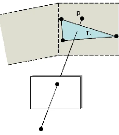
1) The visibility constraint states that the line-of-sight from a camera position to the 3D position of a track seen by this camera belongs to the empty space, i.e., it does not intersect any object in the scene. Therefore a triangle intersected by some line-of-sight should be removed from (see Figure 4a). However, this rule has to be slightly softened to take into account the smoothing step (Section 3.1) where the tracks 3D positions have been slightly changed. More specifically, each trianglet_i in gets a weightw_i equal to the number of lines-of-sight intersecting t_i . We then discard fromany triangle with a weightw_i greater than a threshold

3

 .

2) We also filter out any triangle whose vertices, at least one of them, are only seen by grazing lines-of-sight. In practice, an angle greater than 80 degrees between the line-of-sight and the triangles normal is used in all our experiments to characterise a grazing line-of-sight. 3) Depending on the density of the pre-processed tracks,

the triangle soup can contain “big'' triangles, i.e. triangles whose circumradii are big compared to the

Fig. 4. Visibility constraints: the point p see in the current view has its free space violated by triangle T1 seen in another view.

scale of the scene. We used shape and photo-consistency to filter big triangles.

A triangle is said to be anamorphic if it has a too big radius-edge ratio, where the radius-edge ratio of a triangle is the ratio between the radius of its circumcircle and the length of its shortest edge. Anamorphic big triangles are likely to lie in free space and should be discarded. Big triangles with regular shapes are filtered using photo-consistency criteria: A 3D triangle t_i in  is photo-consistent, if its projections into all images wheret_ivertices are visible correspond to image regions with the same “texture”. To decide on photo-consistency, two common criteria are the Sum of the Squared Difference (SSD) and the Normalised Cross-Correlation (NCC) between pixels inside the projected triangle in each image. In our experiments we use NCC because it is less sensitive to illumination change between the views. We only use images where the angle between the normal of the 3D triangle and the line-of-sight through the centre of the image is small. This scheme gives head-on view more importance than oblique views.

3.3 Reconstruction

For the final step, we use the Delaunay refinement surface mesh generation algorithm [22] described in Section 2. Recall that this algorithm needs to know the surface to be meshed only through an oracle that, given a line segment, detects whether the segment intersects the surface and, if so, returns the intersection points. We implemented the oracle required by the meshing algorithm using the triangles of  as an approximation of the surfaces. Thus, the oracle will test and compute the intersections withto answer to the algorithm queries.

In other words, to produce meshes with different resolutions, we just have to apply the reconstruction step on the extracted triangle soup and alter the Delaunay refinement parameters

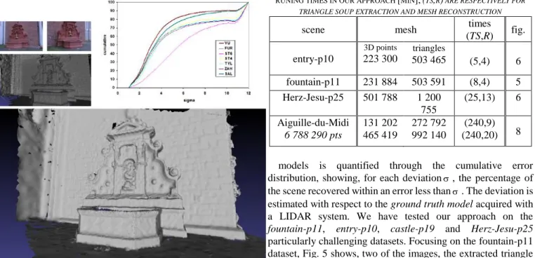
Fig. 5. Top-left: 2 images of fountain-p11 and the extracted triangle soup. Bottom: our reconstruction (500 000 triangles). Top-right: the cumulative error distribution (SAL for our work) compared with VU[16],FUR[14], ST4 [10], ST6 [11],ZAH[31] and TYL[13].

IV. IMPLEMENTATIONANDRESULTS The presented algorithm was implemented in C++, using both CImg and Cgal libraries.

The Cgal library [28] defines all the needed geometric primitives and provides efficient algorithms to compute Delaunay triangulations in both 2D and 3D [29]. It provides a point set processing package [24] needed in the pre-processing step of our algorithm. Moreover, the Cgal library provides access to the AABB tree which is an efficient data structure for intersection detection queries. More importantly it provides us the Delaunay refinement surface meshing algorithm that we use in the last step of our algorithm.

The CImg library [30] is a toolkit for image processing that defines simple classes and methods to manipulate generic images. In our code we use it for the contour detection, the constraint retrieval and the photo-consistency filtering step.

In our experiments, we used for the point cloud pre-processing step the values of parameters (₁;₂;k₁ ;k₂ ), as listed at the end of Section 3.1. Moreover, the visibility constraint threshold

3

 , defined in Section 3.2, is set at 5 rays. Leaving aside the time required by the multi-view stereo processing (image calibration and track extraction), in our experiments the runtime of the reconstruction ranges from 9 minutes for 200 000 tracks on 8 images to 38 minutes for 700 000 tracks on 25 images, on an Intel®Quad Xeon 3.0GHz PC.

Strecha et al. [17] provide quantitative evaluations for six outdoor scene datasets. The evaluation of the reconstructed

TABLE I

scene mesh times

(TS,R) fig. entry-p10 3D points 223 300 triangles 503 465 (5,4) 6 fountain-p11 231 884 503 591 (8,4) 5 Herz-Jesu-p25 501 788 1 200 755 (25,13) 6 Aiguille-du-Midi 6 788 290 pts 131 202 465 419 272 792 992 140 (240,9) (240,20) 8

models is quantified through the cumulative error distribution, showing, for each deviation, the percentage of the scene recovered within an error less than. The deviation is estimated with respect to the ground truth model acquired with a LIDAR system. We have tested our approach on the fountain-p11, entry-p10, castle-p19 and Herz-Jesu-p25 particularly challenging datasets. Focusing on the fountain-p11 dataset, Fig. 5 shows, two of the images, the extracted triangle soup, our reconstruction and the cumulative error distribution compared with the distributions obtained by other reconstructed methods. The stereovision cloud has 392 000 tracks from which 35 percent were eliminated at the pre-processing step. Our algorithm has successfully reconstructed various surface features such as regions of high curvature and shallow details while maintaining a small number of triangles. The comparison with other methods [10, 11, 13, 14, 16, 31] shows the versatility of our method as it generates small meshes that are more accurate and complete than most of the state-of-art while being visually acceptable. Moreover, Fig. 7 illustrates the ability of our algorithm to take into account user-defined size and quality criteria for the mesh facets. Fig. 6 shows our reconstruction results for the entry-p10 and the Herz-Jesu-p25 datasets. For extended results we refer the reader to the challenge website [17].

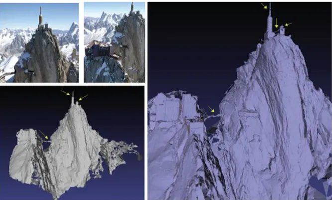
To show the ability of our algorithm to cope with much bigger outdoor scenes and its ability to produce meshes that take into account the user budget for the size of the output mesh, we have chosen to test our method on the Aiguille du Midi dataset (©B.Valet/IMAGINE). It includes 51 images, the extracted cloud has 6 700 000 points with lots of outliers. At the pre-processing step, 80 percent of the points were eliminated. The Delaunay refinement surface meshing is tuned through three parameters: the maximum angle ; the maximum distance between a facet and the surface d and the maximum edge length l. We have tuned parameters d and l to adapt the mesh to a targeted size budget. The reconstructions shown in Fig. 8 are obtained with  equals 20 degrees and the couple (d, l) is set as (0.01, 0.035) and (0.002, 0.01) in unit of the bounding box half diagonal. This enabled us to reconstruct from a single extracted triangle soup output meshes of various resolutions (270 000 triangles and 1 000 000 triangles respectively in Fig. 7). Note that details such as antennas and bridges are recovered even in the coarsest model. Table 1 shows the number of 3D points, the number of triangles for each reconstructed mesh and the time for the reconstruction algorithm.

V. CONCLUSIONANDFUTUREWORK

In this paper, we have proposed a novel 3D mesh reconstruction algorithm combining the advantages of stereovision with the power of Delaunay refinement surface meshing. Visual and quantitative assessments applied on various large-scale datasets indicate the good performance of our algorithm. As for ongoing work, we want to explore the possibility to automatically pre-compute the thresholds such as (₁;₂;₃;k₁ ;k₂ ) from the images and incorporate in the reconstruction process a scale dependent sharp edges detection and recovery procedure to build geometrically simplified models.

ACKNOWLEDGEMENT

We wish to thank Renaud Keriven and Jean-Philippe Pons for their point cloud extraction software and the Aiguille du Midi dataset, Laurent Saboret for his precious collaboration and Christoph Strecha for his challenge and his kind help.

REFERENCES

[1] Ohtake, Y., Belyaev, A., Alexa, M., Turk, G., Seidel, H.P.: Multi-level partition of unity implicits. In: Proc. of ACM SIGGRAPH. (2003) [2] Kazdan, M., Bolitho, M., Hoppe, H.: Poisson Surface Reconstruction. In:

Proc. of SGP’06. (2006)

[3] Hornung, A., Kobbelt, L.: Robust reconstruction of watertight 3D models from non-uniformly sampled point-clouds without normal information. In: Proc. of SGP’06. (2006)

[4] Seitz, S.M., Curless, B., Diebel, J., Scharstein, D., Szeliski, R.: A comparison and evaluation of multi-view stereo reconstruction algorithms. In: Proc. of CVPR’06. (2006)

[5] Seitz, S.M., Dyer, C.R.: Photorealistic scene reconstruction by voxel coloring. In: International Journal of Computer Vision. (1999)

[6] Vogiatzis, G., Torr, P., Cipolla, R.: Multi-view stereo via volumetric graph-cuts. In: Proc. of CVPR’05. (2005)

[7] Pons, J.-P., Keriven, R., Faugeras, O.: Multi-view stereo reconstruction and scene flow estimation with a global image-based matching score. In: International Journal of Computer Vision. (2007)

[8] Pollefeys, M., Nister, D., Frahm, J, Akbarzadeh, A., Mordohai, P., Clipp, B., Engels, C., Gallup, D., Kim, S., Merrell, P.: Detailed real-time urban 3D reconstruction from video. In: International Journal of Computer Vision. (2008)

[9] Zach, C., Pock, T., Bischof, H.: A globally optimal algorithm for robust tv-11 range image integration. In: Proc. of ICCV’07. (2007)

[10] Strecha, C., Fransens, R., Van Gool, L.: Wide-baseline stereo from multiple views: a probabilistic account. In: Proc. of CVPR’04. (2004) [11] Strecha, C., Fransens, R., Van Gool, L.: Combined depth and outlier

estimation in multi-view stereo. In: Proc. of CVPR’06. (2006)

[12] Goesele, M., Snavely, N., Curless, B., Hoppe, H., Seitz, S.: Multi-view stereo for community photo collections. In: Proc. of ICCV’07. (2007) [13] Tylecek, R., Sara, R.: Depth map fusion with camera position refinement.

In: Proc. of CVWW’09. (2009)

[14] Furukawa, Y., Ponce, J.: Accurate, dense and robust multi-view stereopsis. In: Proc. of CVPR’07. (2007)

[15] Pollefeys, M., Van Gool, L., Vergauwen, M., Verbiest, F., Cornelis, K., Tops, J., Kock, R.: Visual modeling with a hand-held camera. In: International Journal of Computer Vision. (2004)

[16] Vu, H., Keriven, R., Labatut, P., Pons, J.-P.: Towards high-resolution large-scale multi-view stereo. In: Proc. of CVPR’09. (2009)

[17] Strecha, C., Von Hansen, W., Van Gool, L., Fua, P., Thoennessen, U.: On benchmarking camera calibration and multi-view stereo for high resolution imagery. In: Proc. Of CVPR’08. (2008) Available:

http://cvlab.epfl.ch/strecha/multiview/denseMVS.html

[18] Hilton, A.: Scene modeling from sparse 3D data. In: Image and Vision Computing. (2005)

[19] Morris, D., Kanade, T.: Image-consistent surface triangulation. In: Proc. of CVPR’00. (2000)

[20] Salman, N., Yvinec, M.: High resolution surface reconstruction from overlapping multiple-views. In: Proc. of SCG’09. (2009)

[21] Salman, N., Yvinec, M.: Surface reconstruction from multi-view stereo. In: Proc. of ACCV’09. (2009)

[22] Boissonnat, J.-D., Oudot, S.: Provably good sampling and meshing of surfaces. In: Graphical Models. (2005)

[23] De Berg, M., Cheong, O., Overmars, M., Van Kreveld, M.: Computational geometry – Algorithms and Applications (3rd). In: Springer-Verlag Berlin. (2008)

[24] Alliez, P., Saboret, L., Salman, N.: Point set processing. In: Board, C.E., ed.: CGAL User and Reference Manual. 3.5 edn. (2009)

[25] Cazals, F., Pouget, M.: Estimating differential quantities using polynomial fitting of osculating jets. In: Proc. of SGP’03. (2003) [26] Canny, J.: A computational approach to edge detection. In: Proc. of

PAMI’86. (1986)

[27] Needleman, S.-B., Wunsch, C.-D.: A general method applicable to the search for similarities in the amino acid sequence of two proteins. In: Journal of Molecular Biology. (1970)

[28] CGAL, Computational Geometry Algorithms Library. Available:

http://www.cgal.org

[29] Boissonnat, J.-D., Devillers, O., Teillaud, M., Yvinec, M.: Triangulations in cgal (extended abstract). In: Proc. of SCG’00. (2000)

[30] CImg, C++ Template Image Processing Toolkit. Available:

http://cimg.sourceforge.net

[31] Zaharescu, A., Boyer, E., Horaud, R.: Transformesh: a topology-adaptive mesh-based approach to surface evolution. In: Proc. of ACCV’07. (2007)

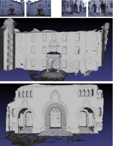
Fig. 6. Top to bottom: 2 images of entry-p10 and 2 images of Herz-Jesu-p25; our reconstruction of entry-p10 (500 000 triangles); our reconstruction of Herz-Jesu-p25 (1 200 000 triangles)

Fig. 7. Fountain-p11 dataset reconstruction: (a-d) 3D meshes resulting from our reconstruction step. By altering the parameters in the reconstruction step, the output mesh becomes coarser, but, the fountain shape remains.

Fig. 8. On the left: two images of the Aiguille du midi dataset (© B.Vallet/IMAGINE); below: our low resolution reconstruction (270 000 triangles). On the right: our high resolution reconstruction (1 000 000 triangles). Note how most details pointed by yellow arrows are recovered in both resolutions.

Nader Salman was born in 1984. He received a Bachelor

in computer science at the University of Nice Sophia Antipolis (UNSA), France, and a M.Sc. in Computer Science on the topic of Image and Geometry for Multimedia and Modelling in life Science at UNSA and Ecole Nationale Supérieure des Telecommunications, France in 2007 with a Master Thesis emphasizing on Synthesis of Compact Textures for Real-time Terrain Rendering. Currently, he is pursuing his PhD thesis in the French national institute for research in computer science and control (INRIA) at Sophia Antipolis, France. His research interests include image-based modelling for the reconstruction of large scale outdoor scenes. Contact him at Nader.Salman@sophia.inria.fr

Mariette Yvinec graduated from Ecole Normale

Supérieure (ENS, Paris) and obtained a phd thesis in solid state physics in 1983.She turned to computer science around 1985 and slightly later, joined the team Geometrica at INRIA Sophia-Antipolis (France). Since then, she published more than 50 journal and conference papers in the field of computational geometry and took an active part in the development of the Computational Geometry Algorithm Library CGAL. She is namely specialist in the fields of triangulations, meshing and their applications to reconstruction. Mariette Yvinec belongs to the editorial board of the Journal of Discrete Algorithms and to the editorial board of CGAL. Contact her at Mariette.Yvinec@sophia.inria.fr