HAL Id: hal-00560881
https://hal.archives-ouvertes.fr/hal-00560881
Submitted on 30 May 2011
HAL is a multi-disciplinary open access
archive for the deposit and dissemination of
sci-entific research documents, whether they are
pub-lished or not. The documents may come from
teaching and research institutions in France or
abroad, or from public or private research centers.
L’archive ouverte pluridisciplinaire HAL, est
destinée au dépôt et à la diffusion de documents
scientifiques de niveau recherche, publiés ou non,
émanant des établissements d’enseignement et de
recherche français ou étrangers, des laboratoires
publics ou privés.
Polytopic control invariant sets for differential inclusion
systems: a viability theory approach
Mirko Fiacchini, Sophie Tarbouriech, Christophe Prieur
To cite this version:
Mirko Fiacchini, Sophie Tarbouriech, Christophe Prieur. Polytopic control invariant sets for
differen-tial inclusion systems: a viability theory approach. ACC 2011 - American Control Conference, Jun
2011, San Francisco, Californie, United States. 8p. �hal-00560881�
Polytopic control invariant sets for
differential inclusion systems: a viability theory approach
Mirko Fiacchini, Sophie Tarbouriech and Christophe Prieur
Abstract— This paper presents a criterion to characterize
control invariant polytopes for differential inclusion systems. The practice-oriented method, based on viability theory and convex analysis, can be applied to determine computational procedures to obtain families of control invariant polytopes. The criterion is based on a necessary and sufficient condition for viability to hold at any point on the boundary of a polytope.
I. INTRODUCTION
The importance of invariance in control and systems analysis has been increasing since the first results on the topic, see the pioneering work [5]. Currently, well established results are available, mainly for linear systems, [15], [18], but also for nonlinear systems [1], [10], [14], see the monograph on invariance [7]. The problem of characterization and com-putation of invariant sets for particular classes of continuous-time nonlinear systems has been tackled in [12], [16], [17], mostly using LMI related approaches. The attention devoted to invariance is strongly due to its tight relation with many basic topics in control and systems analysis, such as stability, domain of attraction estimation and hard constraints satis-faction, among others. On the other hand, few computation-oriented results are available for generic nonlinear systems.
Viability theory, considered from the control point of view, concerns systems whose dynamics are given by a differential inclusion. Roughly speaking, they are systems for which the variation (or the successor, for discrete-time systems) of a state is a set rather than a point in the state space. Viability theory provides mathematical tools to characterize conditions for a set to be robust or control invariant for the system. Viability has been mainly developed by Aubin and co-authors, see [2]–[4], and applies to very general families of sets. See also [9], which proposes methods to construct viability kernels for multi-input single-ouput nonlinear systems affine in the control.
The main objective of this paper is to provide a char-acterization of control invariance and contractiveness of polytopes for differential inclusion systems. As common modeling frameworks, like uncertain systems or constrained controlled ones, can be cast in terms of differential inclusion
This work was partially supported by the ANR project ArHyCo, ARPEGE, contract number ANR-2008 SEGI 004 01-30011459.
M. Fiacchini and S. Tarbouriech are with CNRS; LAAS; 7 avenue du colonel Roche, F-31077 Toulouse, France, Universit´e de Toulouse; UPS, INSA, INP, ISAE; LAAS; F-31077 Toulouse, France. {fiacchini, sophie.tarbouriech}@laas.fr.
C. Prieur is with Department of Automatic Control, Gipsa-lab, Domaine universitaire, 961 rue de la Houille Blanche, BP 46, 38402 Grenoble, France.
systems, the proposed approach applies to a wide class of systems. Differential inclusion can also be used to approx-imate nonlinear systems. In this paper, we focus on linear systems with state-dependent bounds on the input, which are intrinsically nonlinear. It has to be stressed that, while ellipsoidal invariant sets are more common in the context of nonlinear continuous-time systems, results in literature involving polytopes concern mainly linear systems, see [11], [13]. The aim is to apply analytical tools proper of viability theory and convex analysis, see [6], [8], [19], [20], to determine a computation-oriented criterion for characterizing polytopic control invariant sets for constrained continuous-time linear systems. Restricting our attention to polytopes, rather than to the generic sets dealt with in viability theory, allows us to use properties of convex analysis, which lead to tractable problems and more practical solutions. The price to pay is the introduction of a certain conservativeness.
The paper is organized as follows: Section II presents the problem statement, Section III recalls some definitions and results on viability theory. In Section IV the main results on control invariance of a polytope are stated. In Section V the presented method is applied to numerical examples. The paper ends with a section of conclusions.
Notation
Given n ∈ N, define Nn= {x ∈ N : 1 ≤ x ≤ n}. Given A ∈
Rn×m, Aiwith i ∈ Nndenotes its i-th row. Operators ≤, ≥, < and > are intended to apply element-wise to vectors a, b ∈ Rn. Given two sets D and E and a nonnegative scalarα≥ 0, denote the set αD = {αx : x ∈ D}, and the Minkowski set
addition is D ⊕ E = {x = d + e : d ∈ D, e ∈ E}. The interior of D is denoted as int(D), its boundary is ∂D. With S (D)
we denote the set of subsets of D. Given a set valued map F : Rn→ S (Rm), its domain is dom(F) = {x ∈ Rn: F(x) '= /0} and its graph is graph(F) = {(x, y) ∈ Rn× Rm: y ∈ F(x)}.
II. PROBLEM STATEMENT
Consider the continuous-time system given by:
˙x(t) ∈ F(x(t)), (1) where x(t) ∈ Rn is the state at time t, and with F : Rn→
S(Rn), set valued map. Notice that this modeling frame-work, which is referred to as differential inclusion, encloses common systems such as uncertain systems and controlled ones. In fact, the solutions of the uncertain system ˙x(t) =
f (x(t), w(t)), where w(t) ∈ W (x(t)) is the uncertainty (or the
parameter) with W (x) ⊆ Rn, are those of (1) with
Analogously, the trajectories of the controlled system ˙x(t) =
f (x(t), u(t)), with bounds on the input u(t) ∈ U(x(t)) ⊆ Rm,
are those of system (1) with
F(x) = f (x,U(x)) = {y ∈ Rn: y = f (x, u), u ∈ U(x)}. Moreover, differential inclusion can be used to approximate the evolutions of a nonlinear system ˙x(t) = f (x(t)), provided that f (x) ∈ F(x) for all x ∈ Rn.
The objective of this work is to design a computation-oriented method for obtaining polytopic control invariant sets for a controlled system with state-dependent bounds on the input. This means, as formalized below, that our aim is the characterization and computation of a (family of) set K ⊆ Rn
such that, for all x(0) = x0∈ K, there exists an admissible
control signal u(t) ∈ U(x(t)) which permits to maintain the state x(t), solution of (1), in K for t ≥ 0.
III. VIABILITY THEORY
We recall here some general definitions and results on viability theory, which is strongly associated to the research of Aubin and co-authors, see [2]–[4]. Many of those results are developed in the cited works, and references therein, under assumptions which are more general than those re-quired in this paper. Since we are interested in characterizing and computing polytopic control invariant sets, we give the definitions and the properties for the case under analysis.
Definition 1 (Viability properties [3]): Consider the set K ⊆ dom(F). A function x(·) from [0, T ] to Rn, solution of
(1), is called viable if x(t) ∈ K for all [0, T ]. We say that K enjoys the local viability property or control invariance (for the set valued map F) if, for any initial state x0 in K, there
exist T > 0 and a viable solution on [0, T ] to differential inclusion (1). It enjoys the global viability property (or, simply, the viability property) if we can take T = +∞.
Many of the results provided in the context of viability theory analysis are valid for generic nonempty sets K in the state space. An important tool on which those results are based is the contingent cone of set K at x ∈ K, denoted as
TK(x), see [3]. When K is closed and convex, the contingent
cone is equal to the closure of the tangent cone.
Theorem 1 (Tangent cones of closed, convex subsets [3]):
For K ⊆ Rn, closed and convex, its contingent cone TK(x)
coincides with the closure of the tangent cone, given by
Ck(x) =
!
h>0
K − x
h ,
that is the closed cone spanned by K − x.
Then, for convex, closed set K, we have that TK(x) =
CK(x), which are closed and convex cones. Notice that the
tangent cone of a closed, convex set K is Rnat any point x ∈ int(K). Hence, the definition of viability domain, involving the contingent cone in the general case, can be given directly in terms of the tangent cone for closed convex sets.
Definition 2 (Viability domain [3]): Let F : Rn→ S (Rn)
be a nontrivial set valued map. A closed, convex set K ⊆ dom(F) is a viability domain of F if and only if
∀x ∈ K, F(x) ∩CK(x) '= /0. (2)
Also some assumptions on the set valued map F(·) have to be imposed in order to apply the Viability Theorem. A set valued map F : Rn→ S (Rn) fulfilling such assumptions is defined as Marchaud map, which amounts to say that its graph and its domain are closed, the values of F(·) are convex, and the growth of F(·) is linear, see [3]. Such preliminaries are useful since it has been proved that any closed, convex viability domain K for system (1) with F(·) Marchaud map enjoys the viability property.
Theorem 2 (Viability theorem [3]): Consider a Marchaud
map F : Rn→ S (Rn) and a closed, convex K ⊆ dom(F). If
K is a viability domain, then for any state x0∈ K, there exists
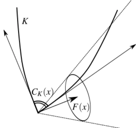
a viable solution on [0, +∞) to the differential inclusion (1). This means that, for every initial condition in K, closed and convex, there exists a trajectory of system (1) which remains in K at any time t ∈ [0, +∞), if there exists a ”direc-tion” belonging to the map F(x(t)) and to the tangent cone of K at x(t), see Figure 1. In this case, in fact, considering such direction at any time, the trajectory would always head towards the interior of set K (or on the boundary).
CK(x)
F(x) K
Fig. 1. Viability condition.
IV. POLYTOPIC CONTROL INVARIANT SETS
The results presented in this section, representing the main contributions of that paper, provide a computation-oriented characterization of control invariance for polytopes.
Consider a polytope in the state space containing the origin in its interior, Ω = {x ∈ Rn: Hx ≤ 1}, with H ∈ Rnh×n, and
the linear controlled system
˙x(t) = Ax(t) + Bu(t), (3) with u(t) ∈ U(x(t)) control input. The input bounding set
U(x(t)) ⊆ Rm is assumed to be the state-dependent polytope
U(x) = {u ∈ Rm: Lu ≤ P(x)}, (4)
with L ∈ Rnu×m and P : Rn→ Rnu, and such that F(x) =
Ax ⊕ BU(x) is Marchaud. Notice that if U(x) is Marchaud
then F(x) = Ax ⊕ BU(x) is Marchaud too, see [3].
Remark 1: No loss of generality is induced by considering
system (3)-(4) in spite of (1). In fact, given F(x) determining (1), Marchaud and with F(x) polytopic, for any A ∈ Rn×nand
defining B = In and U(x) = (−Ax) ⊕ F(x), the differential
inclusion (1) can be written in terms of (3).
The Minkowski function is introduced here, see [7] and references therein for some properties.
Definition 3: Given a compact, convex set K ∈ Rn with
0 ∈ int(K), the Minkowski function of K at x ⊆ Rnis ΨK(x) = min
α≥0{α∈ R : x ∈αK}.
In the case of a polytopic set Ω containing the origin in its interior, the Minkowski function is given by
ΨΩ(x) = min
α≥0{α∈ R : Hjx ≤α,∀ j ∈ Nnh} = maxj∈Nnh{Hjx}.
The objective is to determine a condition for the level sets of the Minkowski function to be control invariant sets, within a region Γ ⊆ Rn. To achieve the purpose, it is sufficient to prove that there exists u(x) ∈ U(x) such that ˙ΨΩ(x) ≤ 0,
for all x ∈ Γ, since it implies that ΨΩ(x) is a nonincreasing
function and since αΩ ⊆βΩ if and only if α ≤β. In what follows we provide conditions, based on the concept of viability, to ensure ˙ΨΩ(x) ≤ 0, which implies that the
level sets of ΨΩ(·) are control invariant sets for system (3)
with constrained input. Furthermore, we aim at determining the greatest region in the state space where such conditions are satisfied and then stability can be ensured by a proper selection of the control input.
Condition ˙ΨΩ(x) ≤ 0 is equivalent to prove that, for every
x ∈ Γ, there exists a u(x) ∈ U(x) such that (Ax + Bu(x)) lies
within the tangent cone of the level set of function ΨΩ(·).
Then, denoted Ω(x) = ΨΩ(x)Ω, the viability condition (2) is
∀x ∈ Γ, (Ax ⊕ BU(x)) ∩CΩ(x)(x) '= /0. (5) Notice that Ω(x) is the smallest level set of ΨΩ(·) containing
x. The tangent cone of Ω(x) at x (which lies on the boundary
of Ω(x), by construction) is given by
CΩ(x)(x) = {v ∈ Rn: Hkv ≤ 0, ∀k ∈ arg max
j∈Nnh{Hjx}}.
Hence, suppose that the state x is known and denote with k =
k(x) ∈ Nnh an index such that Hjx ≤ Hkx for all j ∈ Nnh, that
is, such that Hkx = ΨΩ(x). This is equivalent to k ∈ kΩ(x),
where kΩ(x) ⊆ Nnh is defined as
kΩ(x) = arg max
j∈Nnh{Hjx}. (6)
Given k ∈ Nnh define
Rk= {x ∈ Rn: Hix ≤ Hkx, ∀i ∈ Nnh}, (7)
that is, the region of points x ∈ Rn such that k ∈ k Ω(x).
Notice that regions Rk, with k ∈ Nnh, can have nonempty
intersections. The viability condition (5) is satisfied at x if there exists u = u(x) ∈ U(x) such that
HkAx + HkBu ≤ 0, (8)
for all k ∈ kΩ(x). For every k ∈ Nnh and any x ∈ Rk, as in
(7), we define an optimization problem as follows.
Definition 4 (Primal problem): Consider the system (3)
with input bounds (4). Given k ∈ Nnh and x ∈ Rk, consider
the following optimization problem: αk∗(x) = min α, u α, s.t. Hix ≤α, ∀i ∈ Nnh, τ(HkAx + HkBu) + (Hkx −α) ≤ 0, Lju ≤ Pj(x), ∀ j ∈ Nnu, α≥ 0, (9) withτ>0.
Remark 2: There is no direct connection between the
second inequality in (9) and the Euler Approximating System (EAS), which is a discrete-time system often used in spite of the continuous-time one for computational purposes, see [7]. The inequality has a geometrical meaning, it is valid for every positiveτ and, most importantly, it does not introduce any approximation error. In fact, the condition for viability based on (9) is necessary and sufficient, as illustrated below. A computation-oriented condition for the viability to be satisfied at a point x ∈ Rnstems from the following property.
Proposition 1: Given k ∈ Nnh and x ∈ Rk, the optimal
solution αk∗(x) of the primal problem (9), is such that ΨΩ(x) =αk∗(x) if and only if there exists u ∈ U(x) such that
condition (8) holds at x. Furthermore, ΨΩ(x) <αk∗(x) if and
only if condition (8) is not satisfied at x for any u ∈ U(x).
Proof: First notice that k ∈ kΩ(x) since x ∈ Rk. Suppose
that condition (8) holds for a proper u ∈ U(x). Then the second constraint in (9) is satisfied by the valueα= ΨΩ(x) =
Hkx and the first set of constraints are fulfilled, by definition
of Minkowski function. On the other hand if the optimal value of problem (9) is given by the Minkowski function at x, i.e. αk∗(x) = ΨΩ(x), then the first set of constraints
are satisfied by definition, in fact Hix ≤ maxj∈Nnh{Hjx} =
ΨΩ(x) =α, for all i ∈ Nnh. Moreover, from (6), it follows
that Hkx =α and then the second constraint in (9) becomes
the condition (8). Hence, we can conclude that the solution αk∗(x) is equal to the Minkowski function at x if and only if the condition (8) is satisfied at x.
Furthermore it is easy to see that ΨΩ(x) ≤αk∗(x). In
fact, the value of the Minkowski function at x would be attained by removing the second constraint (if the set U(x) is nonempty, clearly), that means, it would be the optimal over a greater feasibility region, and then a smaller or equal value should be obtained. Hence it can be concluded that the optimal solution of the optimization problem is equal to the Minkowski function at x if and only if condition (8) is satisfied at x. This implies that the optimal value is greater than ΨΩ(x) if and only if (8) is not fulfilled at x.
In what follows, we are going to use the Lagrange multi-pliers and the dual optimization problem to pose geometric conditions for a region of the state space to be a control invariant set. First, it is worth recalling that for the case under analysis strong duality holds if the primal is feasible, being (9) a linear problem in the optimization variables α and u, see [6], [8].
opti-mization problems and defining the function Lk(β,δ,σ; x) = nh
∑
i=1 βiHix +δ τHkAx +δHkx − nu∑
j=1 σjPj(x),we obtain the dual problem:
L∗k(x) = max β ,δ ,σ Lk(β,δ,σ; x), s.t. nh ∑ i=1βi+δ≤ 1, δ τHkB + nu ∑ j=1σjLj= 0, β≥ 0, δ ≥ 0, σ≥ 0, (10)
whose optimal value is such that Lk(β,δ,σ; x) ≤ L∗k(x) for all feasible (β,δ,σ), clearly. Hence L∗k(x) is the maximal lower bound of αk∗(x) and, from strong duality, L∗
k(x) =αk∗(x).
Then, Lk(β,δ,σ; x) ≤αk∗(x) for any feasible solution of (10).
Proposition 2: A necessary and sufficient condition for
inequality (8) to be satisfied at x ∈ Rk is
L∗k(x) ≤ Hkx, (11)
or, equivalently Lk(β,δ,σ; x) ≤ Hkx for every feasible
solu-tion (β,δ,σ) of (10). Furthermore, condition (8) is violated at x ∈ Rk if and only if
L∗k(x) > Hkx, (12)
or, equivalently, if there exists a feasible solution (β,δ,σ) of (10) such that Lk(β,δ,σ; x) > Hkx.
Proof: Recall that ΨΩ(x) ≤αk∗(x) and that ΨΩ(x) <αk∗(x)
if and only if (8) does not hold at x ∈ Rk. Then (8) holds
at x if and only if Hkx = ΨΩ(x) = L∗k(x) =αk∗(x), which
is implied by (11). Analogously, it can be proved that (12) entails that αk∗(x) > ΨΩ(x) and then, as previously shown,
violation of condition (8).
Posing the condition for viability as in (11), rather than by means of an equality constraint, permits to obtain convex optimization problems under adequate assumptions on U(x). Consider now the dual problem (10). Given k ∈ Nnh and
x ∈ Rk, the problem is the maximization of a linear function
over a polyhedral set in the space of variablesβ,δ andσ. In general case, the maximum is attained at some extreme point or the problem is unbounded. Since the primal optimum exists and is bounded, the analysis can be reduced to the extreme points of the feasibility region of the dual problem.
Property 1: The optimal value of the dual problem (10)
is attained at an extreme point of the feasibility region.
Proof: Since the origin is an extreme point of the
fea-sibility region of the dual problem (10), which is bounded above by the primal optimal value, the result is implied by Fundamental Theorem of Linear Programming, see [6].
It is important to stress the fact that the feasibility region of the dual problem does not depend on the value of x but only on Hk(and on the structure of the system, clearly). Then
the dual problem feasibility set is valid for every x ∈ Rk and
its extreme points can be precomputed knowing Hk only.
Proposition 3: Given k ∈ Nnh, denote with (β
p,δp,σp)
the p-th extreme point of the feasibility region of the dual
problem (10), with p ∈ Nnv. The subset of Rk, defined in
(7), such that the condition (8) is satisfied at x ∈ Rk by a
u(x) ∈ U(x) is given by
Vk= "
p∈Nnv
{x ∈ Rn: Lk(βp,δp,σp; x) ≤ Hkx}. (13)
Furthermore, the region of points x ∈ Rk for which the
condition (8) is violated for every u ∈ U(x) is ¯
Vk= !
p∈Nnv
{x ∈ Rn: Lk(βp,δp,σp; x) > Hkx}. (14)
Proof: From Property 1 we have that, for every x ∈ Rk,
there exists a p∗= p∗(x) ∈ N
nv such that
Lk(β,δ,σ; x) ≤ Lk(βp
∗
,δp∗,σp∗; x) = L∗k(x), for any feasible (β,δ,σ). From this and Proposition 2 the first claim follows. Analogous considerations prove the second claim.
It is worth stressing that Vk, given by the intersection of
subsets of the state space, is the exact region of all x ∈ Rk
where condition (8) is satisfied for an adequate u(x) ∈ U(x). The only optimization problem to solve for characterizing Vk concerns the computation of the extremes of the dual problem, neither the computation of u(x) is required.
Remark 3: Notice that Vk is the set of points in Rk for
which condition (8) is satisfied by a u = u(x) ∈ U(x), for a particular k ∈ kΩ(x). This is equivalent to the condition of
viability for all x ∈ int(Rk), that is if kΩ(x) = {k}. Viability, in
fact, should concern a condition on u ∈ U(x) involving every
k ∈ kΩ(x). Intriguing phenomena (as Zeno solutions, for
instance) could occur at x ∈∂Rk, with k ∈ Nnh, and deserve
more accurate considerations. The analysis of such boundary phenomena is one the objective of our future research.
From the computational point of view, it is important to notice that if Pj(x) is concave in x for all j ∈ Nnu,
the functions Lk(βp,δp,σp; x) are convex and then Vk is
a convex set. Analogously, if Pj(x) is convex in x for all
j ∈ Nnu, then the Lk(βp,δp,σp; x) is a concave function and
¯
Vkis a union of convex sets. The analysis of the different nh regions Rk, one for any Hk with k ∈ Nnh, permits to obtain
a polytopic viable domain.
V. ILLUSTRATIVE EXAMPLES
Example 1: Consider the linear system (3) with matrices A = # 0 −1 1 0 $ , B = # 1 0 0 1 $ , (15) and constraints on the input is U(x) = U = {u ∈ R2:
-u-∞≤
1}. The trajectories in absence of control are given by the circumferences of the circles centered in the origin. It is, then, immediate to check that any circle in the state space is a viable set for the dynamic system. On the other hand, our aim here is to use this simple explanatory example to illustrate how the proposed results can be used for computing a family of control invariant sets and a region where viability condition holds for Ω(x).
Consider the set Ω = {x ∈ R2: -x-1≤ 1}. The objective
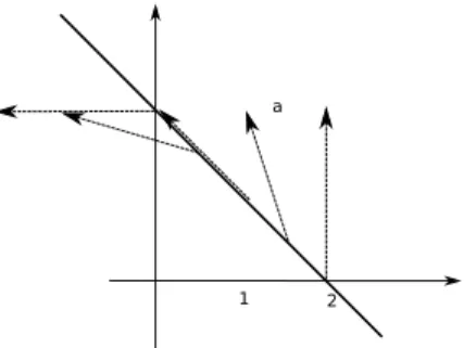
Fig. 2. Autonomous directions on the boundary ofγΩ in R1.
control invariant polytopes for everyµ such that 0 ≤µ≤γ. Considering Hk= [1 1], the region under analysis is the first
quadrant, i.e. Rk= {x ∈ R2: x ≥ 0}. By geometric inspection
it can be noticed that the ”critical” point in Rk for viability
ofγΩ is x = [γ 0]T, see Figure 2. Actually, moving x along the facet of γΩ from [γ 0]T to [0 γ]T, the direction of the autonomous system, i.e. Ax, is such that HkAx decreases,
becoming negative from x = [0.5γ 0.5γ]T. Notice that if
HkAx ≤ 0 then viability condition holds at x simply posing
u = [0 0]T. By geometric inspection it can also be concluded that the maximal γk for which γkΩ satisfies the viability
condition in the region Rkisγk= 2, see Figure 3. We expect
to recover the same value applying the presented results.
2 1 3 Ax Ax Ax ⊕ U Ax ⊕ U
Fig. 3. SetsγΩ and system dynamics.
The dual problem feasibility region for the case under analysis is given by the following constraints:
δ τ+σ1−σ3= 0, δ τ+σ2−σ4= 0, nh ∑ i=1βi +δ≤ 1, β≥ 0, δ≥ 0, σ≥ 0.
Notice that, for any possible value ofδ, there exist admissi-ble values ofσ such that the linear equality constraints hold. The first constraint, for instance, is satisfied by every pair of valuesσ3≥ 0 andσ1≥ 0 such that their difference is equal to
δ τ. The extreme values ofβ andδ are given by the extreme points of the region, in their subspace, contained between the simplex and the origin. Then the extreme values ofδ are 0 or 1. Forδ= 0 we have thatσis such thatσ1=σ3andσ2=σ4,
and then the extremes are σ1=σ3= 0 or σ1=σ3= +∞
andσ2=σ4= 0 orσ2=σ4= +∞. The infinite values can
be discarded, since the related function Lk(β,δ,σ; x) would
be equal to −∞, then leading to trivial inequalities in the definition of Vk and ¯Vk, (see (13) and (14)). Then the only
interesting extremes are given by σi = 0, for i ∈ N4. The
other possibility isδ = 1 and then the finite extreme value ofσ isσ= [0 0τ τ]T. Thus the finite extreme values of the dual problem feasibility region are
(β1,δ1,σ1) =) 1 0 0 0 0 0 0 0 0 *T, (β2,δ2,σ2) =) 0 1 0 0 0 0 0 0 0 *T, (β3,δ3,σ3) =) 0 0 1 0 0 0 0 0 0 *T, (β4,δ4,σ4) =) 0 0 0 1 0 0 0 0 0 *T, (β5,δ5,σ5) =) 0 0 0 0 1 0 0 τ τ *T, (β6,δ6,σ6) =) 0 0 0 0 0 0 0 0 0 *T. The resulting set of (nontrivial) constraints determining x ∈
Rk such that the viability condition holds for Ω(x) are
Lk(β1,δ1,σ1; x) = [1 1]x ≤ [1 1]x, Lk(β2,δ2,σ2; x) = [1 − 1]x ≤ [1 1]x, Lk(β3,δ3,σ3; x) = [−1 1]x ≤ [1 1]x, Lk(β4,δ4,σ4; x) = [−1 − 1]x ≤ [1 1]x, Lk(β5,δ5,σ5; x) = [1 1]x +τ[1 − 1]x − 2τ≤ [1 1]x, Lk(β6,δ6,σ6; x) = 0 ≤ [1 1]x, and then x2≥ 0, x1≥ 0, [−1 − 1]x ≤ 0, [1 − 1]x ≤ 2. (16)
The region Vk, and the half-spaces that determine it as in
(16), are depicted in Figure 4. The shadowed regions are those points in the state space that violate constraints (16), and then the white portion of the space represents Vk. Thus,
the maximalγk such thatγkΩ satisfies the viability condition
in Rk is 2, as expected. From symmetry, analogous results
are obtained for every Ri, with i ∈ N4, and the resultingγ,
obtained as the minimalγi, is 2. It is important to stress that
no extreme point computation for Ω is required, the half-space representation of the polytope is sufficient.
Example 2: We consider now the same continuous-time
dynamic system (15), with state-dependent bounds on the control input, that is U(x) = {u ∈ R2: Lu ≤ P(x)} with
L = 1 0 0 1 −1 0 0 −1 , P = −x2 1+ 16 −x2 2+ 9 −x2 1+ 9 −x22+ 4 .
Thus, the bounds on the input are boxes whose extreme values dependent on the state. Notice that the bounds are tighter as the state is further from the origin. We have to expect, then, that viability condition is satisfied in a region around the origin. Moreover, since Pj(·) are concave
in x, then functions Lk(β,δ,σ; ·) are convex and then the
viable region Vk is also convex, being the intersection of
convex sets. Functions Lk(βp,δp,σp; x) are the same as in
the previous example for all p '= 5. For p = 5 the convex constraint results in:
[1 1]x +τ[1 − 1]x −τ(−x2
1− x22+ 13) ≤ [1 1]x,
⇔ x2
1+ x22+ x1− x2− 13 ≤ 0. (17)
Constraints and the region Vk are depicted in Figure 5.
Fig. 5. Viability region in Rk.
The points where the circumference of (17) intersects the axis are [3.14 0]T, [−4.14 0]T, [0 3.14]T and [0 − 4.14]T.
The result can be checked from a geometric point of view. In fact, consider the point ˆx = [3.14 0]T and the set valued
map at this point. The input bounding set at ˆx is given by
U( ˆx) = {u ∈ R2: 0.86 ≤ u1≤ 25.86, −4 ≤ u2≤ 9}
and A ˆx = [0 3.14]T. Then the vector v( ˆx) = [0.86 − 4]T is
admissible, i.e. v( ˆx) ∈ U( ˆx), and A ˆx+ v( ˆx) lies in the tangent cone of Ω( ˆx) = 3.14Ω at ˆx, as depicted in Figure 6.
VI. CONCLUSIONS
The paper presented a method to characterize control invariance of polytopes for differential inclusion systems. Properties related to viability theory and to convex sets and functions have been used to propose a practice-oriented method for analysis and computation of control invariant polytopes. Several problems and possible directions of fur-ther research are open, such as the analysis of border phenomena like Zeno solutions, the characterization of poly-hedral Lyapunov functions and the problem of control design.
Fig. 6. Critical point of viability region in R1.
REFERENCES
[1] T. Alamo, A. Cepeda, M. Fiacchini, and E. F. Camacho. Convex invariant sets for discrete–time Lur’e systems. Automatica, 45:1066– 1071, 2009.
[2] J.-P. Aubin. A survey of viability theory. SIAM Journal of Control and Optimization, 28(4):749–788, 1990.
[3] J.-P. Aubin. Viability theory. Birkh¨auser, 1991.
[4] J.-P. Aubin and H. Frankowska. Set-valued analysis. Birkh¨auser, 1990. [5] D. P. Bertsekas. Infinite-time reachability of state-space regions by using feedback control. IEEE Transactions on Automatic Control, 17:604–613, 1972.
[6] D. P. Bertsekas, A. Nedic, and A. E. Ozdaglar. Convex analysis and optimization. Athena Scientific, 2003.
[7] F. Blanchini and S. Miani. Set-Theoretic Methods in Control. Birkh¨auser, 2008.
[8] S. Boyd and L. Vandenberghe. Convex Optimization. Cambridge University Press, 2004.
[9] M. E. Broucke and J. Turriff. Viability kernels for nonlinear control systems using bang controls. IEEE Transactions on Automatic Control, 55:1280–1284, 2010.
[10] M. Cannon, V. Deshmukh, and B. Kouvaritakis. Nonlinear model predictive control with polytopic invariant sets. Automatica, 39:1487– 1494, 2003.
[11] E. B. Castelan and J. C. Hennet. On invariant polyhedra of continuous-time linear systems. IEEE Transactions on Automatic Control, 38(11):1680–1685, November 1993.
[12] W. H. Chen, D. J. Ballance, and J. O’Reilly. Optimisation of attraction domains of nonlinear MPC via LMI methods. In Proc. of the IEEE American Control Conference, Arlington, VA, USA, 2001.
[13] L. Farina and L. Benvenuti. Invariant polytopes of linear systems. IMA Journal of Mathematical Control and Information, 15:233–240, 1998.
[14] M. Fiacchini, T. Alamo, and E.F. Camacho. On the computation of convex robust control invariant sets for nonlinear systems. Automatica, 46(8):1334–1338, 2010.
[15] E. G. Gilbert and K. Tan. Linear systems with state and control constraints: The theory and application of maximal output admissible sets. IEEE Transactions on Automatic Control, 36:1008–1020, 1991. [16] J. M. Gomes da Silva Jr. and S. Tarbouriech. Antiwindup design with guaranteed regions of stability: an LMI-based approach. IEEE Transactions on Automatic Control, 50(1):106–111, jan. 2005. [17] T. Hu and Z. Lin. Exact characterization of invariant ellipsoids
for single input linear systems subject to actuator saturation. IEEE Transactions on Automatic Control, 47(1):164 –169, jan 2002. [18] I. Kolmanovsky and E. G. Gilbert. Theory and computation of
dis-turbance invariant sets for discrete-time linear systems. Mathematical Problems in Engineering, 4:317–367, 1998.
[19] R. T. Rockafellar. Convex Analysis. Princeton University Press, USA, 1970.
[20] R. Schneider. Convex bodies: The Brunn-Minkowski theory, vol-ume 44. Cambridge University Press, Cambridge, England, 1993.