HAL Id: tel-01227582
https://hal.inria.fr/tel-01227582
Submitted on 11 Nov 2015
HAL is a multi-disciplinary open access archive for the deposit and dissemination of sci-entific research documents, whether they are pub-lished or not. The documents may come from teaching and research institutions in France or abroad, or from public or private research centers.
L’archive ouverte pluridisciplinaire HAL, est destinée au dépôt et à la diffusion de documents scientifiques de niveau recherche, publiés ou non, émanant des établissements d’enseignement et de recherche français ou étrangers, des laboratoires publics ou privés.
Roberto Amadini
To cite this version:
Roberto Amadini. Portfolio Approaches in Constraint Programming. Computer Science [cs]. Univer-sity of Bologna, 2015. English. �tel-01227582�
DOTTORATO DI RICERCA IN INFORMATICA
Ciclo: XXVII
Settore Concorsuale di afferenza: 01/B1
Settore Scientifico disciplinare: INF/01
Portfolio Approaches in
Constraint Programming
Candidato: Roberto Amadini
Coordinatore Dottorato:
Relatore:
Maurizio Gabbrielli
Maurizio Gabbrielli
Recent research has shown that the performance of a single, arbitrarily efficient algorithm can be significantly outperformed by using a portfolio of —possibly on-average slower— algorithms. Within the Constraint Programming (CP) context, a portfolio solver can be seen as a particular constraint solver that exploits the synergy between the constituent solvers of its portfolio for predicting which is (or which are) the best solver(s) to run for solving a new, unseen instance.
In this thesis we examine the benefits of portfolio solvers in CP. Despite portfolio approaches have been extensively studied for Boolean Satisfiability (SAT) problems, in the more general CP field these techniques have been only marginally studied and used. We conducted this work through the investigation, the analysis and the construction of several portfolio approaches for solving both satisfaction and optimization problems. We focused in particular on sequential approaches, i.e., single-threaded portfolio solvers always running on the same core.
We started from a first empirical evaluation on portfolio approaches for solving Constraint Satisfaction Problems (CSPs), and then we improved on it by introduc-ing new data, solvers, features, algorithms, and tools. Afterwards, we addressed the more general Constraint Optimization Problems (COPs) by implementing and testing a number of models for dealing with COP portfolio solvers. Finally, we have come full circle by developing sunny-cp: a sequential CP portfolio solver that turned out to be competitive also in the MiniZinc Challenge, the reference competition for CP solvers.
“Gratus animus est una virtus non solum maxima, sed etiam mater virtutum omnium reliquarum”1
Marcus Tullius Cicero.
Writing acknowledgements is more difficult than it looks. There is always some-one that you forget to mention, and probably those people will be among the few that will read the acknowledgements. It is not just a selection task, but also a scheduling problem: you do not have to only choose the people to thank, but even who thank first and who later.
Let us begin by winding the timeline back about three years ago. If I have could join the Ph.D. program, part of the credit can be taken by Prof. Gianfranco Rossi —who introduced me to Constraint (Logic) Programming and also supervised my Bachelor and Master theses— and Prof. Roberto Bagnara, both professors at the University of Parma, which wrote the reference letters needed for the application.
Once I started the Ph.D. program, I had the opportunity to know friendly and easygoing colleagues with whom I shared the moments of hopelessness and satis-faction typical of every Ph.D. student. Among them, I would like in particular to mention: Gioele Barabucci, Luca Bedogni, Flavio Bertini, Luca Calderoni, Or-nela Dardha, Angelo Di Iorio, Jacopo Mauro, Andrea Nuzzolese, Giulio Pellitta,
1 “Gratitude is not only the greatest of virtues, but the parent of all others”.
Almost all the work described in this thesis has been conducted together with Prof. Maurizio Gabbrielli, the Ph.D. program coordinator as well as my supervisor, and with Dr. Jacopo Mauro.
Let me say that it is not uncommon to hear about Ph.D. students treated as employees, if not servants, by their supervisors. On the contrary, Maurizio is a very good man and has been for me an ideal supervisor: he never put pressure on me, leaving me almost total freedom of research.
Jacopo introduced me to Algorithm Portfolios, and has been the colleague that most helped me during the doctorate course. We had sometimes lively debates, but without his help it would have been very difficult to get the appreciable results we achieved during these years.
During my Ph.D. program I also had a really enjoyable staying at the NICTA (National ICT of Australia) Optimisation Research Group of Melbourne. In this regard I would like to thank all the members of the group, and in particular: Dr. Andreas Schutt, who helped me on some technical issues and also reviewed this thesis; Prof. Peter J. Stuckey, my supervisor overseas, who gave me valuable and interesting insights, and Alessandra Stasi, the group coordinator, for her precious help on logistics and bureaucracy.
My sincere thanks to the reviewers of this thesis, Dr. Andreas Schutt and Prof. Eric Monfroy, for their detailed and in-depth reviews and for their useful and infor-mative comments.
I can say that these three years have been for me a positive turning point, not only from the academic point of view. Many thanks to those who helped me to achieve this goal, with apologies to those I have not mentioned above.
Il dottorato di ricerca `e il massimo grado di istruzione universitaria ottenibile. Si tratta senza ombra di dubbio di un traguardo significativo, una pietra miliare nel percorso di crescita —non solo professionale— di una persona. Al di l`a dei dovuti ringraziamenti di rito, il mio grazie pi`u grande va a coloro che pi`u di tutti hanno contribuito al raggiungimento di questo titolo. Parlo ovviamente dei miei genitori, Bruno e Tiziana.
Abstract iii
Acknowledgements v
1 Introduction 1
1.1 Outline . . . 3
2 Constraint Programming 7 2.1 Constraint Satisfaction Problems . . . 8
2.1.1 CSP on Finite Domains . . . 11 2.1.1.1 Boolean Variables . . . 11 2.1.1.2 Integer Variables . . . 13 2.1.1.3 Other Variables . . . 14 2.1.2 CSP Solving . . . 15 2.1.2.1 Consistency techniques . . . 16
2.1.2.2 Propagation and Search . . . 17
2.1.2.3 Nogood Learning and Lazy Clause Generation . . . . 18
2.1.2.4 Local Search . . . 19
2.2 Constraint Optimization Problems . . . 20
2.2.1 Soft Constraints . . . 21
2.2.1.1 Fuzzy Constraints and Weighted CSPs . . . 22 ix
2.2.2.1 Linear Programming . . . 24
2.2.2.2 Nonlinear Programming . . . 25
3 Portfolios of Constraint Solvers 29 3.1 Dataset . . . 31 3.2 Solvers . . . 33 3.3 Features . . . 34 3.4 Selectors . . . 36 3.5 Related Work . . . 38 4 Portfolios of CSP Solvers 41 4.1 A First Empirical Evaluation . . . 42
4.1.1 Methodology . . . 43 4.1.1.1 Dataset . . . 43 4.1.1.2 Solvers . . . 44 4.1.1.3 Features . . . 45 4.1.1.4 Validation . . . 46 4.1.1.5 Portfolios composition . . . 49 4.1.1.6 Off-the-shelf approaches . . . 49 4.1.1.7 Other approaches . . . 51 4.1.2 Results . . . 54
4.1.2.1 Percentage of Solved Instances . . . 54
4.1.2.2 Average Solving Time . . . 58
4.1.2.3 Summary . . . 59
4.2 An Enhanced Evaluation . . . 60
4.2.1 SUNNY: a Lazy Portfolio Approach . . . 61
4.2.1.1 SUNNY Algorithm . . . 62 x
4.2.2.2 Solvers . . . 68
4.2.2.3 Features . . . 70
4.2.3 Results . . . 73
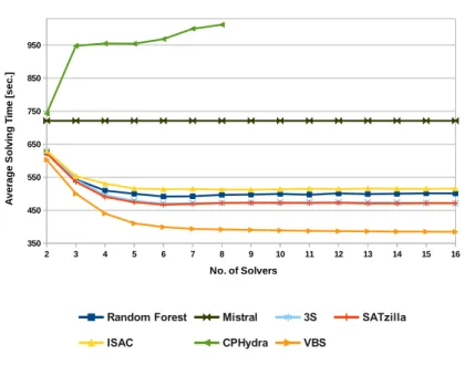
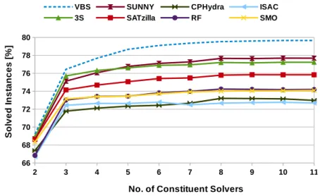
4.2.3.1 Percentage of Solved Instances . . . 74
4.2.3.2 Average Solving Time . . . 75
4.2.3.3 sunny-csp . . . 77
4.2.3.4 Training Cost . . . 80
4.2.3.5 Summary . . . 82
5 Portfolios of COP Solvers 85 5.1 An Empirical Evaluation of COP Portfolio Approaches . . . 86
5.1.1 Evaluating COP solvers . . . 87
5.1.1.1 The score function . . . 89
5.1.2 Methodology . . . 92
5.1.2.1 Solvers, Dataset, and Features . . . 92
5.1.2.2 Portfolio Approaches . . . 93
5.1.3 Results . . . 96
5.1.3.1 Score . . . 97
5.1.3.2 Optima Proven . . . 100
5.1.3.3 Optimization Time . . . 101
5.1.3.4 MiniZinc Challenge Score . . . 102
5.1.3.5 Summary . . . 104
5.2 Sequential Time Splitting and Bound Communication . . . 105
5.2.1 Solving Behaviour and Timesplit Solvers . . . 105
5.2.2 Splitting Selection and Evaluation . . . 108
5.2.2.1 Evaluation Metrics . . . 109 xi
5.2.3 Timesplit Portfolio Solvers . . . 116 5.2.3.1 Static Splitting . . . 118 5.2.3.2 Dynamic Splitting . . . 120 5.2.4 Empirical Evaluation . . . 120 5.2.4.1 Test Results . . . 123 5.2.4.2 Summary . . . 126
6 sunny-cp: a CP Portfolio Solver 129 6.1 Architecture . . . 130
6.1.1 Usage . . . 133
6.2 Validation . . . 136
6.3 Summary . . . 142
7 Conclusions and Extensions 145
References 149
Introduction
“Dimidium facti, qui coepit, habet”1
Quintus Horatius Flaccus.
The Constraint Programming (CP) paradigm is a general and powerful frame-work that enables to express relations between different entities in form of con-straints that must be satisfied. The concept of constraint is ubiquitous and not confined to the sciences: constraints appear in every aspect of daily life in the form of requirements, obligations, or prohibitions. For example, logistic problems like task scheduling or resource allocation can be addressed by CP in a natural and el-egant way. The CP paradigm, characterized as a sub-area of Artificial Intelligence, is essentially based on two vertical layers:
(i) a modelling level, in which a real-life problem is identified, examined, and formalized into a mathematical model by human experts;
(ii) a solving level, aimed at resolving as efficiently and comprehensively as possible the model defined in (i) by means of software agents called constraint solvers. 1 “Well begun is half done”.
The goal of CP is to model and solve Constraint Satisfaction Problems (CSPs) as well as Constraint Optimization Problems (COPs) [159]. Solving a CSP means to find a solution that satisfies all the constraints of the problem. A COP is instead a generalized CSP where we are also interested in optimal solutions, i.e., solutions that minimize a cost or maximize a payoff.
The Algorithm Selection (AS) problem, for the first time formalized by John R. Rice in 1976 [157], can be roughly reduced to the following question:
Given an input problem P and a set A = {A1, A2, . . . , An} of algorithms,
which is the “best” algorithm Ai ∈ A for solving problem P ?
The underlying idea behind AS is very general and implicitly used in practical ev-eryday human problems. For instance, let us suppose the problem P is “I have to go from place x to place y” and the algorithm space is A = {“Go from x to y by M ” : M ∈ {car, train, plane}}. The selection necessary depends on the input problem parameters x and y: e.g., if we have to move from Bologna to Melbourne, the choice is obvious and strongly dominated by the the distance between x and y. Less clear would be instead the choice if x = “Bologna” and y = “Roma”. Here other problem features must be taken into account: e.g., the possible heavy traffic in the raccordo anulare of Roma2, or the remote possibility of train strikes or delays. Moreover, note that the definition of “best” algorithm is not self-contained and generally bound to a performance metric: the best path from x is to y is the shortest, the fastest, the cheaper, or what?
According to [118] definition, Algorithm Portfolios [103] can be seen as partic-ular instances of the more general AS problem in which the algorithm selection is performed case-by-case instead that in advance. In this case, a portfolio of algo-rithms corresponds to the algorithm space A. The concept of portfolio comes from Economics, and refers to a collection of financial assets used for maximizing the ex-pected return and minimizing the overall risk of having just a single stock. Within the Artificial Intelligence field, algorithm portfolios have been deeply investigated
by Gomes and Selman [83, 82, 84]. Within the sub-area of CP the algorithm space is constituted by a portfolio {s1, s2, . . . , sm} of different constraint solvers si. We
can thus define a portfolio solver as a particular constraint solver that exploits the synergy between the constituent solvers of its portfolio. When a new unseen prob-lem p comes, the portfolio solver tries to predict which is (or which are) the best constituent solver(s) s1, s2, . . . , sk (k ≤ m) for solving p and then runs such solver(s)
on p.
The goal of this thesis is to examine the benefits of portfolio approaches in Constraint Programming. From this perspective the state of the art of portfolio solvers is still a raw fruit if compared, e.g., to the SAT field where a number of effective portfolio approaches have been developed and tested. We constructed, analysed and evaluated several portfolio approaches for solving generic CP problems (i.e., both CSPs and COPs). We started with satisfaction problems, then we moved to optimization ones and finally we have come full circle by developing sunny-cp: a portfolio solver for solving generic CP problems that turned out to be competitive also in the MiniZinc Challenge [176, 177], the reference competition for CP solvers. A more detailed outline of the contents and the contributions of this thesis is reported in the next section.
1.1
Outline
This thesis is conceptually organized in three main parts. The first part (Chapters 2 and 3) contains the background notions about CP and portfolio solvers. The second one (Chapters 4 and 5) presents detailed and extensive evaluations on portfolio approaches applied to CSPs and COPs respectively. The last part describes the sunny-cp tool (Chapter 6) and concludes the thesis by reporting also the ongoing and future works (Chapter 7). Hereinafter we show an outline of these chapters.
Chapter 2 provides an overview of Constraint Programming: the main do-mains, solving techniques, and approaches for solving both CSPs and COPs.
namely: the dataset of instances used to make (and test) predictions, the constituent solvers of the portfolio, the features used to characterize each problem, and the techniques used to properly select and execute the constituent solvers.
Chapter 4 presents an extensive investigation on CSP portfolio solvers. We started from an initial empirical evaluation, where we compared by means of simu-lations some state-of-the-art portfolio solvers against some simpler approaches built on top of some Machine Learning classifiers. Then we report a more extensive eval-uation in which, in particular, we introduce SUNNY: a new algorithm portfolio for constraint solving.
Chapter 5 shifts the focus on optimization solvers. We first formalized a suitable model for adapting the “classical” satisfaction-based portfolios to address COPs, providing also some metrics to measure the solver performance. Then, we simulated and evaluated the performances of different COP portfolio solvers. After this work, we take a step forward by assessing the benefits of sequential time splitting and bounds communication between different COP solvers.
Chapter 6 describes sunny-cp: a sequential CP portfolio solver that can be run just like a regular single constraint solver. We show the overall architecture of sunny-cp and we assess its performance according to the good results it achieved in the MiniZinc Challenge 2014.
Chapter 7 concludes the thesis by providing some insights and final remarks on the work we have done, we are doing and we are planning to do.
Summarizing, the contributions of the thesis are the followings:
• we built solid baselines by performing several empirical evaluations of different portfolio approaches for solving both CSPs and COPs;
• we provided —by means of proper tools— the full support of MiniZinc, nowa-days a de-facto standard for modelling and solving CP problems, while still retaining the compatibility with XCSP format;
• we developed SUNNY, a lazy portfolio approach for constraint solving. SUN-NY is a simple and flexible algorithm portfolio that, without building an
ex-plicit prediction model, predicts a schedule of the constituent solvers for solving a given problem.
• we took a step forward towards the definition of COP portfolios. We intro-duced new metrics and studied how CSP portfolio solvers might be adapted to deal with COPs. In particular, we addressed the problem of boosting opti-mization by exploiting the sequential cooperation of different COP solvers; • we finally reaped the benefits of our work for developing sunny-cp: a portfolio
solver aimed at solving a generic CP problem, regardless of whether it is a CSP or a COP. To the best of our knowledge, sunny-cp is currently the only sequential portfolio solver able to solve generic CP problems.
Some of the contributions of this thesis have already been published. Most of the work in Chapter 4 has been published in [7, 8, 10]. A journal version of [7] is currently under revision. Chapter 5 mostly report the papers published in [9, 12]. A journal version of [9] is currently under revision. Chapter 6 presents an extended version of [11]. Papers [7, 8, 10, 9, 11] are joint works with Dr. Jacopo Mauro and Prof. Maurizio Gabbrielli, in which I contributed as primary author. Paper [12] was co-written with Prof. Peter J. Stuckey.
Constraint Programming
“Constraint Programming represents one of the closest approaches Computer Science has yet made to the Holy Grail of programming: the user states the problem, the computer solves it.” Eugene C. Freuder.
Constraint programming (CP) is a declarative paradigm wherein relations be-tween different entities are stated in form of constraints that must be satisfied. The goal of CP is to model and solve Constraint Satisfaction Problems (CSPs) as well as Constraint Optimization Problems (COPs) [159]. A CSP consists of three key components:
• a finite set of variables, i.e., entities that can take a value in a certain range; • a finite set of domains, i.e., the possible values that each variable can take; • a finite set of constraints, i.e., the allowed assignments to the variables. Solving a CSP means finding a solution, i.e., a proper assignment of domain values to the variables that satisfies all the constraints of the problem. COPs can be instead regarded as generalized CSPs where we are interested in finding a solution that minimizes (or maximizes) a given objective function. The resolution of these problems is performed by software agents called constraint solvers. Henceforth, if not further specified, with the term “CP problem” we will refer to either a CSP or
a COP. Analogously, the term “CP solver ” will refer to a constraint solver able to solve both CSPs and COPs.1
CP appeared in the 1960s in systems such as Sketchpad [70], and core ideas such as arc and path consistency techniques were proposed and developed in the 1970s. The real landmark of CP was in the 1980s with the coming of Constraint Logic Pro-gramming (CLP), a form of CP which embeds constraints into logic programs [20]. The first implementations of CLP were Prolog III, CLP(R), and CHIP. Another paradigm for solving hard combinatorial problems that has its foundations in logic programming is the Answer-Set Programming (ASP) [128]. Apart from logic pro-gramming, constraints can be mixed with other paradigms such as functional and imperative. Usually, they are embedded within a specific programming language or provided via separate software libraries.
Constraint Programming combines and exploits a number of different fields in-cluding for example Artificial Intelligence, Programming Languages, Combinatorial Algorithms, Computational Logic, Discrete Mathematics, Neural Networks, Opera-tions Research, and Symbolic Computation. The applicaOpera-tions of CP cover different areas: scheduling and planning are probably the most prominent ones, but con-straints may also be considered for problems of configuration, networking, data mining, bioinformatics, linguistics, and so on. This chapter provides an overview of some of the main concepts and techniques used in the CP field.
2.1
Constraint Satisfaction Problems
In this section, after giving the basic notions of CSP and some examples, we provide an overview of the most common domain and the main solving techniques.
1 Note that the borderline between CSP and COP solvers is fuzzy. Indeed, since a COP is a
generalization of a CSP, a solver able to solve COPs can also solve CSPs. However, a CSP solver can solve a COP by enumerating and ranking every solution it finds. We however maintain this categorization since the different nature and solving techniques between CSPs and COPs.
Definition 2.1 (CSP) A Constraint Satisfaction Problem (CSP) is a triple P := (X , D, C) where:
• X := {x1, x2, . . . , xn} is a finite set of variables;
• D := D1× D2× · · · × Dn is a n-tuple of domains such that Di is the domain
of variable xi for each i = 1, 2, . . . , n;
• C := {C1, C2, . . . , Cm} is a finite set of constraints with arity 0 ≤ k ≤ n
defined on subsets of X . More formally, if C ∈ C is defined on a subset of variables {xi1, xi2, . . . , xik} ⊆ X then C ⊆ Di1 × Di2 × · · · × Dik.
Definition 2.2 (Satisfiability) Let d := (d1, d2, . . . , dn) ∈ D be a n-tuple of
do-main values. It is said that d satisfies a constraint C ∈ C defined on variables {xi1, xi2, . . . , xik} if and only if (di1, di2, . . . , dik) ∈ C. A constraint C is satisfiable
if and only if there exists at least a d ∈ D that satisfies C (otherwise C is said unsatisfiable). A tuple d ∈ D is a solution of a CSP if and only if d satisfies every C ∈ C. If a CSP has at least a solution is said satisfiable (otherwise, is said unsatisfiable).
Given a CSP P := (X , D, C) the goal is normally to find a solution of P, that is, a n-tuple (d1, d2, . . . , dn) ∈ D of domain values that satisfies every c ∈ C.2 To better
clarify the above definitions, consider the following examples.
Example 2.1 (Send More Money) The problem “ Send More Money” is a clas-sical crypto-arithmetic game published in the July 1924 issue of Strand Magazine by Henry Dudeney. The objective is to unequivocally associate to each letter l ∈ {S, E, N, D, M, O, R, Y } a digit dl ∈ {0, 1, . . . , 9} so that the equation SEN D +
M ORE = M ON EY is met. This problem can be mapped to a CSP P := (X , D, C) where:
• X := {x1, x2, . . . , x8}, where the variable xi corresponds to the i-th element of
the vector x = hS, E, N, D, M, O, R, Y i;
• D := D1× D2× · · · × D8 = {0, 1, . . . , 9} × {0, 1, . . . , 9} × · · · × {0, 1, . . . , 9};
• C := {C1, C2, C3}, where:
– C1 := {(d1, d2, . . . , d8) ∈ D | d1 > 0 ∧ d5 > 0},
i.e., the most significant digits S and M must not be zero; – C2 := {(d1, d2, . . . , d8) ∈ D | di 6= dj for 1 ≤ i < j ≤ n},
i.e., all the variables in X must be distinct;
– C3 := {(d1, d2, . . . , d8) ∈ D | 1000d1 + 100d2+ 10d3+ d4+
1000d5+ 100d6+ 10d7+ d2 =
10000d5+ 1000d6+ 100d3 + 10d2+ d8},
i.e., the equation SEN D + M ORE = M ON EY must be satisfied.
This problem is satisfiable: its (unique) solution is d = (S, E, N, D, M, O, R, Y ) = (9, 5, 6, 7, 1, 0, 8, 2).
Example 2.2 (n-Queens) The n-Queens problem consists in positioning n > 3 queens on a chessboard n × n in such a way that none of them can attack each other. This problem can be modelled by a CSP P := (X , D, C) with:
• X := {x1, x2, . . . , xn}, where xi = j if and only if the i-th queen is placed on
the j-th column of the chessboard. Note that since a variable can assume only one value, this also implies that it is not possible to place two queens on the same row; • D := D1× D2× · · · × Dn= {1, 2, . . . , n} × {1, 2, . . . , n} × · · · × {1, 2, . . . , n}; • C :=S 1≤i,j≤n{C 0 ij, C 00 ij} where:
– Cij0 := {(d1, d2, . . . , dn) ∈ D | di 6= dj}, i.e, no queens on the same column;
– Cij00 := {(d1, d2, . . . , dn) ∈ D | |di− dj| 6= i − j} i.e, no queens on the same
For example, if n = 4 there are two solutions: d1 = (2, 4, 1, 3) and d2 = (3, 1, 4, 3).
However, since they differ only by a rotation on the chessboard, these solutions can actually be seen as a single one. Indeed, in the n-Queens problem there is plenty of symmetries, i.e., solutions that are identical up to symmetry operations (rotations and reflections). Symmetries occur naturally in many problems, and it is very important to deal with them to avoid wasting time to visit symmetric solutions, as well as parts of the search tree which are symmetric to already visited parts. Two common types of symmetry are variable symmetries (which act just on variables), and value symmetries (which act just on values) [43]. One simple but highly effective mechanism to deal with symmetry is to add constraints which eliminate symmetric solutions [47]. An alternative way is modify the search procedure to avoid visiting symmetric states [59, 76, 158, 63].
2.1.1
CSP on Finite Domains
Constraints can be of different types according to the domain of the variables in-volved. For example, if p, q, r are Boolean variables we could express constraints of the form r ≡ p ∨ q or p ∧ q → r. If n is an integer variable and X, Y are set variables, we could consider a constraint of the form |X ∩ Y | ≤ n which constrains X and Y to have at most n common elements. Although in theory there is no limitation on the domains of the variables (e.g., they could be discrete, continuous, or symbolic) the most successful CP applications are based on Finite Domains (FD), i.e., the domain of the variables has finite cardinality. This section provides an overview of the most widely used FD in Constraint Programming.
2.1.1.1 Boolean Variables
In CSPs with only Boolean variables, each variable can be set to either true or false. The most common class of Boolean CSPs is represented by (Boolean, Propositional) Satisfiability problems, better known as SAT problems [87]. In these problems the goal is to determine if there exists an interpretation (i.e., an assignment of Boolean
values to the variables) that satisfies a given Boolean formula.
Historically, the SAT problem was the prototype and one of the simplest NP-complete problems [45]. It attracted a lot of attention throughout the years, and nowadays is probably the area of greatest influence in the context of satisfiabil-ity problems. SAT solving is commonly used in many real life problems such as automated reasoning, computer-aided design and manufacturing, machine vision, database, robotics, integrated circuit design, computer architecture design, and computer network design. Its widespread use has fostered the dissemination of a large number of different solvers [81], which success is probably due to the com-bination of different techniques like nogoods, backjumping, and variable ordering heuristics [142]. In particular, as we will see below, SAT solving is the CSP branch in which portfolio approaches have been grown more. Starting from 2002, interna-tional SAT solver competitions [111] take place in order to evaluate the performance of different solvers on extensive benchmarks of real case, randomly generated and hand-crafted instances defined in the Dimacs standard format [112]. It is worth not-ing that, although technically SAT problems are simplified CSPs, in the literature there is a clear distinction between them and the ”generic“ CSPs (which typically have integer domains). This is because of the different nature between SAT solving and other approaches like FD solving or Linear Programming. Henceforth, if not better specified, with the term CSP we will refer only to generic CSPs, excluding from such categorization the SAT problems.
There is plenty of SAT variants and related problems like 2-SAT, 3-SAT, HORN-SAT, XOR-SAT. In particular, the Maximum Satisfiability problem (MAX-SAT) [21] is the problem of finding an interpretation that satisfies the maximum number of clauses. A well-known extension of SAT is Satisfiability Modulo Theories (SMT) [19] that enriches SAT formulas with linear constraints, arrays, all-different constraints, uninterpreted functions, and so on. These extensions typically remain NP-complete, but efficient solvers are developing to handle such types of constraints. The SAT problem becomes harder if we allow both existential ∃ and universal ∀ quantifica-tion: in this case, it is called Quantified Boolean Formula problem (QBF) [35]. In
particular, the presence of the ∀ quantifier in addition to ∃ makes the QBF problem PSPACE-complete.
2.1.1.2 Integer Variables
For most of the problems is more natural to model a CSP with integer variables belonging to a finite range (e.g., [−1..5] = {−1, 0, . . . , 5}) or to a disjoint union of finite ranges (e.g., [2..8] ∪ [10..20]).3 Usually, a CSP over integers supports some
standard basic constraints (like =, 6=, <, ≤, >, ≥, +, −, ·, /, . . . ) together with global constraints. A global constraint [159] can be seen as a constraint over an arbitrary sequence of variables. The most common global constraints usually come with spe-cific algorithms (the so-called propagators) that may help to solve a problem more efficiently than decomposing the global constraint into basic relations. This feature is perhaps one of the main strengths of FD solvers when solving huge combinatorial search problems. The canonical example of a global constraint is the all-different constraint. An all-different constraint over a set of variables states that the vari-ables must be pairwise different. This constraint is widely used in practice and because of its importance is offered as a built-in constraint in the large majority of commercial and research-based constraint programming systems. In fact, although from a purely logic point of view the semantic of all-different (x1, x2, . . . , xn) is the
same of the logic conjunction V
1≤i,j≤nxi 6= xj, the use of a specific propagator can
make the resolution dramatically more efficient. Other examples of widely applicable global constraints are the global cardinality constraint (gcc) [156] or the cumulative constraint [5]. An exhaustive list of global constraints can be retrieved at [24].
Differently from SAT field, in CSP context there are fewer and less stable solvers (e.g., see the number of entries in SAT solver competitions [25] w.r.t. CP solver competitions [110, 139]). It should be noted that SAT problems are much easier to encode: a CSP may contain more complex constraints (e.g., global constraints 3Note that in the literature the term ”FD solver“ refers almost always to a solver operating
on integer variables, possibly equipped with additional extensions (e.g., finite sets of integers). Moreover, sometimes the terms ”FD solver“ and ”CP solver“ are used as synonyms.
like bin-packing or regular ). Moreover, at the moment the CP community has not yet agreed on a standard language to encode CSP instances. The XML-based lan-guage XCSP [161] was used to encode the input problems of the International CSP Solver Competition (ICSC) [109]. XCSP is still used but, since the ICSC ended in 2009, its spread over recent years has been restricted. At present, the de-facto standard for encoding (not only) CSP problems is MiniZinc [146]. MiniZinc is cur-rently the most used, supported, and general language to specify CP problems. It supports also optimization problems and is the source format used in the MiniZ-inc Challenge (MZC) [176], which is nowadays the only international competition for evaluating the performances of CP solvers. MiniZinc is a medium-level language that reduces the overall complexity of the higher-level language Zinc [135] by remov-ing user-defined types, various coercions, and user-defined functions. Unlike XCSP, MiniZinc provides the separation between model and data, is not restricted to in-tegers, it allows if-then-else constructs, arrays, loops, varied global constraints, and more recently it added new features like user-defined functions and option types. FlatZinc [22] is a low-level language which is mostly a subset of MiniZinc. It is designed for translating a general model into a specific one that has the form re-quired by a particular solver. Indeed, starting from a solver-independent MiniZinc model every solver can produce its own FlatZinc model by using solver-specific re-definitions. Apart from MiniZinc, other solver-independent modelling languages are ESRA [62], Essence [68], and OPL [180].
2.1.1.3 Other Variables
In the last years, researchers have given special attention to set variables and con-straints. Many complex relations can be expressed with set constraints such as set inclusion, union, intersection, disjointness, cardinality. An example of a logic-based language for set constraints is CLP(SE T ) [55]. It provides very flexible and gen-eral forms of sets, but its effectiveness is hindered by its solving approach, which is strongly non-deterministic. More recently, other approaches were proposed to deal with finite sets of integers. Common ways to represent the domain of a set variable
are the subset-bounds representation [17] and the lexicographic-bounds representa-tion [163]. A radically different approach based on the Reduced Ordered Binary Decision Diagrams (ROBDDs) is proposed in [95], an integration between BDD set solvers and SAT solvers is described in [96], and a framework for combining set variable representation is shown in [28]. Note that some FD solvers prefer to not use set constraints, since it is possible to get equivalent formulations by making use of only binary or integer variables.
With regard to the domain of rational and real numbers, some approaches have been proposed especially in the context of CLP. For example, CLP(Q, R) system [99] was developed to deal with linear (dis)equations over rational and real numbers. A separate mention concerns instead the floating-point domain. Solving constraints over floating-point numbers is a critical issue in numerous applications, notably in program verification and testing. Albeit the floating-point numbers are a finite sub-set of the real numbers, classical CSP techniques are here ineffective since the huge size of the domains and the different properties of floating-point numbers w.r.t. real numbers. In [137] a solver based on a conservative filtering algorithm is proposed. In [32] the authors addressed the peculiarities of the symbolic execution of pro-grams with floating-point numbers, while [23] proposes to use Mixed Integer Linear programming for boosting local consistency algorithms over floating-point numbers. The flexibility and generality of the CSP framework makes however possible its ex-tension to non-standard domains. For example, CSPs have also been defined over richer data types like multi-sets (or bags) [117, 182], graphs [54], strings [80] and lattices [61].
2.1.2
CSP Solving
As mentioned earlier, solving a CSP means assigning to each variable a consistent value of its domain. Intuitively, a trivial technique could be the systematic explo-ration of the solutions space. This approach, also referred as “Generate & Test”, is based on a simple idea: a complete assignment of values to variables is iteratively generated until a (possible) solution is found. Obviously, despite this algorithm
guarantees the completeness of the search on finite domains, it becomes intractable very quickly when increasing the problem size. There are two main ways to improve the efficiency of this approach: using a ”smart“ assignments generator, so as to minimize the failures in the test phase; and merging the generator with the tester, which is the way of CSP solving. In the last case, the consistency is tested as soon as variables are instantiated by using a backtracking approach [136].
Backtracking is a general approach that tries to build a solution by incrementally exploring the branches of the search space in order to extend the current partial solu-tion (initially empty). When an inconsistency is detected, the algorithm abandons that path and backtracks to a consistent node, thus eliminating a subspace from the Cartesian product of the domains. Despite this pruning allows to improve the Generate & Test approach, the running complexity of backtracking is still NP-hard for most non-trivial problems. The three major drawbacks of standard backtracking are: thrashing (i.e., repeated failures due to the same reason), redundant work (i.e., the conflicting values of variables are not remembered), and late detection (i.e., the conflict is not detected before it really occurs). We now present an overview of some of the major enhancements of the backtracking approach. A formal and detailed descriptions of the following methods is outside the scope of this thesis: for more details we refer the reader to the corresponding references.
2.1.2.1 Consistency techniques
A well-known approach for solving CSPs is based on consistency techniques. The basic consistency techniques are based on the so called constraint (hyper) graph —sometimes called constraints network— where nodes correspond to variables and (hyper) edges are labelled by constraints.
Several consistency notions are reported in the literature [125, 129]. Let us fix a problem P := (X , D, C). The simplest consistency technique is the node-consistency (NC), which requires that for every variable xi ∈ X , every unary constraint C
on {xi}, every d ∈ Di, we have that d ∈ C. The most widely used consistency
pair of variables xi, xj, every binary constraint C on {xi, xj}, every value d ∈ Di,
there exists a value d0 ∈ Dj such that (d, d0) ∈ C . Even more invalid values can
be removed by enforcing the path-consistency (PC). Path-consistency requires that for every triplet of variables xi, xj, xk, every C on {xi, xj}, every C0 on {xi, xk}, and
every C00 on {xj, xk}, if (d, d0) ∈ C then it exists a d00 ∈ Dk such that (d, d00) ∈ C0
and (d0, d00) ∈ C00.
It can be shown that the above consistency techniques are covered by a gen-eral notion of (strong) k-consistency [66]. Indeed, NC is equivalent to strong 1-consistency, AC to strong 2-1-consistency, and PC to strong 3-consistency. Algo-rithms exist for making a constraint graph strongly k-consistent for k > 2, but in practice they are rarely used because of efficiency issues. Note that virtually all the consistency algorithms are not complete: in other terms, meeting a given notion of consistency does not imply that the CSP is really consistent. This is because achieving the completeness can be computationally very hard: from the practical perspective it is preferable to settle for relaxed forms of consistency that do not eliminate the need for search in general, but however allow to remove efficiently a significant amount of inconsistencies.
2.1.2.2 Propagation and Search
Even if both systematic search and consistency techniques might be used alone to completely solve CSPs, this is rarely done: a combination of both approaches is a more common way of solving. According to a given notion of local consistency, for each different kind of constraint suitable agents called propagators are responsible to remove the inconsistent values in order to meet such consistency notion. A local removal may trigger other propagators which in turn may remove values from other domains (e.g., consider the CSP in the Example 2.3).
Example 2.3 Consider a CSP P with three variables x, y, z having domains Dx :=
[0..1], Dy := [−6..1], Dz := {1, 5} and with two constraints {x < y, y 6= z}. P is
node-consistent, but not arc-consistent. For example, if x = 1 then no value of Dy
reasonably assigns the values 0 to x and 1 to y; this narrowing affects y 6= z, which becomes 1 6= z. Then, the propagator of 6= removes 1 from Dz and consequently
assign the value 5 to z.
The process of propagation is iterated until a fix-point is reached; this can happen when the domain of a variable becomes empty (i.e., the CSP is unsatisfiable) or no further values can be removed (i.e., the consistency notion is met). Unfortunately, since consistency techniques are usually incomplete, there is no guarantee that once a fix-point is reached the CSP is actually consistent. To overcome this limitation, it is necessary to perform a search in the solutions space for to verify if there exists a consistent assignment of values to variables. This process can be done either by considering all the variables of X , or by performing and checking the assignments on a proper subset L ⊂ X of so-called “labelled” variables. Different search heuristics can be adopted and combined to speed up the search (e.g., variable choice heuristics and value choice heuristics).
2.1.2.3 Nogood Learning and Lazy Clause Generation
In order to avoid some problems of backtracking, like thrashing and redundant work, look-back schemes like backjumping [71] or backchecking [94] were proposed. Typically look back schemes share the disadvantage of late detection of the conflict: they solve the inconsistency when it occurs but do not prevent the inconsistency to occur. Therefore, look-ahead schemes were proposed to prevent future conflicts. Forward checking is the easiest example of a look-ahead strategy.
A very effective technique for preventing conflicts and reducing the search space consists in learning conflicts during the search [51]. In the SAT context this is better known as clause learning. The development and the refinement of clause learning techniques has led to dramatic improvements for SAT solving [142]. The equivalent of clause learning in CSP field is called nogood learning. Nogoods are redundant constraints that in [51] are technically defined as variable assignments that are not contained in any admissible solution. They can be learned during search, stored, and used to prune further part of the search tree. In [115] the authors pointed out
that nogood learning in CSP has not been as successful as clause learning in SAT, and also proposed a generalization of standard nogoods.
There exists a lot of work proposing different techniques for encoding a CSP into a SAT problem [4, 104, 18, 178, 174]. A hybrid approach, called Lazy Clause Gener-ation, is instead presented in [149]. Lazy clause generation combines the strengths of CP propagation and SAT solving. The key idea is to mimic the underlying rules of FD propagators by properly generating corresponding SAT clauses. The clause generation is ”lazy“ since it is not performed a priori, but it occurs during the search. This approach enables a strong nogood learning, able to detect and analyse the conflicts that occur during the search. Benefits of lazy clause generation on the RCPSP/max problem are shown in [168]. Moreover, the lazy clause generation solver Chuffed [78] has dominated the MiniZinc Challenges 2012–2014.
2.1.2.4 Local Search
The large size and the heterogeneous nature of real-world combinatorial problems make it sometimes impracticable the use of exact approaches. A possible workaround consists in using Local Search (LS) methods. LS methods are greedy approaches based on a simple and general idea: trying to improve a current ”local“ solution by moving from time to time toward a possibly better solution within a given neigh-bourhood. If there are not better solutions in the neighbourhood, it means that a local optimum was reached. To avoid getting stuck in a local optimum, several effective techniques can be applied.
In [65] different hybrid methods are reported for combining the efficiency of LS with the flexibility of CP paradigm. Some local search methods (e.g., [39, 49, 148, 152]) used CP as a way to efficiently explore large neighbourhoods with side constraints. Others, such as [40], used LS as a way to improve the exploration of the search tree.
In the particular context of the CSPs, a LS approach iteratively tries to improve an assignment of the variables until all the constraints are satisfied. The local search is therefore performed in the space D of the possible assignments, by means of a
proper evaluation function for measuring the quality of the assignments (e.g., in terms of the number of violated constraints).
Two main classes of local search algorithms exist. The first one is that of greedy or non-randomized algorithms. Well-known examples of greedy algorithms are the Hill Climbing [169] and the Tabu Search [79]. The main drawback of these algo-rithms concerns the possibility of getting stuck in a sub-optimal state. To over-come this problem, randomized LS algorithms has been devised. Examples of such random-walk algorithms are the the WalkSAT/GSAT [170] and the Simulated An-nealing [181].
2.2
Constraint Optimization Problems
In many real-life applications we are not just interested in finding ”a” solution but “the” optimal solution, or at least a good one. The quality of the solutions is usually measured by an application-dependent function called objective function which can represent a cost as well as a gain. The goal is no longer just finding a solution, but finding one that minimizes or maximizes the objective function. These kinds of problems are referred to as Constraint Optimization Problems (COPs)4.
From now on, without loss of generality, we will always consider a COP as a minimization problem. Indeed, it is always possible to switch from a maximization problem to an equivalent minimization problem by simply negating the objective function. Formally, a COP can be defined as follows:
Definition 2.3 (COP) A Constraint Optimization Problem (COP) is a qua-druple P := (X , D, C, f ) where:
• P0 := (X , D, C) is a CSP;
• f : D → R is the objective function of P.
The goal is normally to find a solution of P0 that minimizes f . Clearly, a COP is more general than a CSP (that can be instead regarded as a particular COP in which f is constant over D). For instance, a solution d found by a COP solver can be sub-optimal (i.e., there exists at least a better solution d0 < d). Moreover, a COP solver may find an optimal solution d∗ without being able to prove its optimality.5
Well-known examples of COPs are for instance the Cutting-stock problem [90] (essentially reducible to the Bin-packing and Knapsack problems), the Vehicle Rout-ing Problem (VRP) (introduced in [48] as a generalization of the TravellRout-ing Salesman Problem (TSP) [64]), and the Resource-Constrained Project Scheduling Problem (RCPSP) [34].
A widely used algorithm for solving COPs is called Branch and Bound (BB). This method was first proposed in [126] for discrete programming, and has become the most commonly used tool for solving combinatorial optimization problems. A BB procedure consists essentially in two steps. The branching step recursively splits the original problem into sub-problems or, in other terms, splits the search tree into sub-trees. The bounding step instead estimates the lower and upper bounds of the objective function f over each sub-problem. The key idea of BB algorithm is: if the lower bound for a sub-problem P1 is greater than the upper bound for another
sub-problem P2, then P1 can be safely discarded from the search (pruning).
In the rest of the section we focus in particular on two aspects of constrained op-timization: the so-called Soft Constraints, and the Operations Research techniques for dealing with constrained optimization.
2.2.1
Soft Constraints
When a large set of constraints needs to be solved, it is not unlikely that there is no way to satisfy them all: the problem is said to be over-constrained. Moreover, it
5
Normally, for CP solvers the codomain of f is a finite subset of N. However, in case of non-finite domains, a COP solver should also be able to prove the unboundedness of a problem. For example, let us consider a simple COP defined by P := ({x}, Z, ∅, f (x) := −x). In this case P is unbounded, since f (x) is unbounded in Z.
could be that several solutions are equally optimal. This can be caused by an inap-propriate modelling: constraints are used to formalize desired properties rather than preferences (i.e., conditions whose violation should be avoided as far as possible). Soft constraints provide a way to model the preferences. In this section, inspired by [159], we provide an overview of the most important classes and techniques of soft constraints.
2.2.1.1 Fuzzy Constraints and Weighted CSPs
There are many classes of soft constraints. The Fuzzy Constraints approach is based on the Fuzzy Set Theory [57, 56]. Fuzzy constraints map the preferences in a range between 0 (total rejection) and 1 (complete acceptance). The preference of a solution is computed by taking the minimal preference over the constraints. This may seem counter-intuitive in some scenarios, but it is instead more natural in others. For example, in critical settings like medical applications we would like to be as cautious as possible. Probabilistic constraints [165] and fuzzy lexicographic constraints [60] are variants of classical fuzzy constraints.
In other contexts we are more interested in the damages we get by not satisfy-ing a constraint, rather than in the advantages we obtain when we satisfy it. In Weighted Constraint Satisfaction Problems (WCSPs) each constraint is provided with a weight representing the penalty to be paid when such constraint is violated. An optimal solution is therefore a solution that minimizes the sum of the weights of the violated constraints. If all the weights are set to 1, we get the MAX-CSP problem [67]: similarly to the MAX-SAT problem, here the goal is maximizing the number of satisfied constraints. Weighted constraints are among the most expres-sive soft constraint frameworks, since fuzzy constraint problems can be efficiently reduced to weighted constraint problems [166].
2.2.1.2 Formalism and Inference
The literature contains at least two general formalisms to model soft constraints: semiring-based constraints [29, 30] and valued constraints [166]. Semiring-based
constraints rely on a simple algebraic structure which is very similar to a semi-ring. Valued constraints depend instead on a positive totally ordered commutative monoid and use a different syntax w.r.t. semiring-based constraints. However, if we assume preferences to be totally ordered [31], they have the same expressive power. Soft constraint problems are as expressive, and as difficult to solve, as constraint optimization problems. Indeed, given any soft constraint problem we can always build a COP with the same solution ordering, and vice versa.
Inference in soft constraints reflects the same basic notions of classical con-straints. Bucket elimination (BE) [52, 53] is a complete inference algorithm which is able to compute all the optimal solutions of a soft constraint problem. The high memory cost is the main drawback of using BE in practice. Because complete infer-ence can be extremely time and space intensive, it is often more interesting to use simpler but more efficient techniques of soft constraint propagation.
2.2.2
Optimization and Operations Research
In a nutshell, Operations Research (OR, also called Operational Research) is the discipline of applying advanced analytical methods to help make better decisions. Operations Research originated in the efforts of military planners during World War II, and subsequently largely adopted for civilian purposes in a huge variety of fields including business, finance, logistics, and government. OR encompasses a wide range of problem-solving techniques and methods applied in the pursuit of improved decision-making and efficiency, such as simulation, mathematical op-timization, queueing theory and other stochastic-process models, Markov decision processes, econometric methods, data envelopment analysis, neural networks, ex-pert systems, decision analysis, and the analytic hierarchy process.6 In particular,
COPs are well studied and used in practice in areas such as services, logistics, trans-ports, economics, and in many other industrial applications. Operations research has proved to be useful for modelling problems of planning, routing, scheduling,
assignment, and design. In this section we provide an overview of the classical OR optimization methods and a comparison between CP and OR techniques.
2.2.2.1 Linear Programming
Linear programming (LP) is a general OR optimization method in which both the constraints and optimization function are linear. The canonical form of a LP prob-lem is:
maximize cTx
subject to Ax ≤ b, x ≥ 0
where x ∈ Rn is the vector of the variables to be assigned, c ∈ Rn and b ∈ Rm
are vectors of known coefficients (cT is the transpose of c) while A ∈ Rm×n is the
matrix of the constraints coefficients. The inequalities Ax ≤ b are constraints that specify a convex polyhedron (the feasible region) over which the objective function f (x) = cTx has to be maximized.
Every LP problem (or linear program), referred to as a primal problem, can be converted into a corresponding dual problem, which provides an upper bound to the optimal value of the primal problem [33]. Note that the dual of a dual linear program is the original primal linear program. Given the above definition of primal problem, the corresponding dual is:
minimize bTy
subject to ATy ≥ c, y ≥ 0
The theory of the duality shows some interesting properties (e.g., the duality theo-rems) and it is also exploited by the simplex algorithm [144]. This method, devised by George Dantzig in 1947, makes use of the concept of simplex (i.e., a polytope of n + 1 vertices in n dimensions) for solving LP programs. Other effective techniques for solving LP problems are instead based on interior point methods [153].
The general LP framework can be specialized according to the variables domain. For instance, if all of the variables are required to be integers it is called an Integer
Linear Programming (ILP) problem. In contrast to LP, which can be solved effi-ciently in the worst case, ILP problems are in many practical situations (those with bounded variables) NP-hard. A special case of ILP where variables are constrained to be either 0 or 1 is the Binary Integer Programming (BIP, also called 0-1 integer programming). Despite the binary domain of the variables, this problem is also classified as NP-hard. If only some of the variables are required to be integers, then the problem is called a Mixed Integer Programming (MIP) problem. These are gen-erally NP-hard because they are even more general than ILP programs. However, despite the NP-hardness, some important subclasses of ILP and MIP problems are efficiently solvable. In addition to BB, other advanced algorithms for solving LP problems include for instance the cutting-plane method and the column generation.
2.2.2.2 Nonlinear Programming
In contrast to LP, in Nonlinear Programming (NLP) problems some of the con-straints or the objective function are nonlinear. Formally, an NLP program has the following form:
minimize f (x)
subject to gi(x) = 0 for i = 1, 2, . . . , m
and hj(x) ≥ 0 for j = m + 1, m + 2, . . . , n
where n ≥ 0 is the total number of constraints of the problem, 0 ≤ m ≤ n is the num-ber of equalities and at least one function in {f, g1, g2, . . . , gm, hm+1, hm+2, . . . , hn}
is nonlinear.
A well-known subclass of NLP problems is constituted by the Quadratic Pro-gramming (QP) problems. A QP problem is the problem of optimizing a quadratic function subject to linear constraints. Formally, it can be formulated as:
minimize 1
2x
TQx + cTx
subject to Ax ≤ b
where x ∈ Rn represents the vector of variables; b ∈ Rm, c ∈ Rn, and d ∈ Rp are vectors of known coefficients while A ∈ Rm×n, E ∈ Rp×n and Q ∈ Rn×n are matrices
of known coefficients (in particular, Q is symmetric).
A related programming problem, called Quadratically Constrained Quadratic Programming (QCQP), can be posed by adding quadratic constraints on the vari-ables. For general QP problems a variety of methods are commonly used, including interior point, active set [143], augmented Lagrangian [44], conjugate gradient, gra-dient projection, extensions of the simplex algorithm [143]. QP is particularly simple when only equality constraints appear. If Q is a positive definite matrix, the ellipsoid method solves the problem in polynomial time [123].
Operating Research vs. Constraint Programming
Roughly speaking, Operating Research and Constraint Programming can be re-garded as different approaches for solving hard combinatorial problems. Both of these techniques has strengths as well as weaknesses, for which reason it is not pos-sible to determine which is the best technique to be adopted in general. As often happens in Computer Science, some algorithms work very well on a certain class of problems, but are ineffective for others. In these cases, often the best solution is to use a hybrid approach able to merge the strengths of the different algorithms. CP and OR have indeed complementary strengths: on the one hand CP provides an easy way to deal with inference methods, logic processing, high-level problem mod-elling and local consistency; on the other, OR works well with relaxation methods, duality theory, atomistic problem modelling, and global consistency. Consequently, in order to achieve better performances and solve large combinatorial problems, it has become natural try to integrate these two approaches and the links between the two communities have grown stronger in recent years [138].
The general advantages of CP consist in being better at sequencing and schedul-ing, in the more natural modellschedul-ing, in the use of global constraints, and in a natural way to locally control the constraints. In contrast, CP paradigm is usually weaker when treating discrete and continuous variables as well as over-constrained and
op-timization problems. Moreover, this field is younger and less explored if compared to OR. Some experimental results show that a hybrid methodology allows to signif-icantly outperform both CP and OR for various classes of problems (e.g., planning and scheduling-based problems) [100].
The emerging research field of the integration between OR techniques and CP is promising and stimulating. Some of the main challenges concern the interaction between the user and the solving process, the resolution of partially unknown or ill-defined problems, the processing of large scale over-constrained problems, and the improvement of the CP solving process, both in the constraints propagation and in the solution search [138].
Portfolios of Constraint Solvers
“Multae Manus Onus Levant”1
It is well recognized in the field of Artificial Intelligence, but we could say in Computer Science in general, that different algorithms have different performance when solving different problems (even belonging to the same class). As pointed out also by the “No Free Lunch” theorems [184, 185] it is evident that a single algorithm can not be a panacea for all possible problems. Given a problem x and a collection of different algorithms A1, A2, . . . , Am, the Algorithm Selection (AS) problem basically
consists in selecting which algorithm Ai performs better on x.
The AS problem was introduced by John R. Rice in 1976 [157]. An overall diagram of the (refined) model he proposed is depicted in Figure 3.1. Given an input problem x, a proper vector f (x) of real valued features is first extracted from x. Features are essentially instance-specific attributes that characterize a given problem. Dealing with features is crucial in AS: the idea is selecting, via a proper selection mapping S, the best algorithm A = S(f (x)) for problem x on the basis of the feature vector f (x). The notion of “best algorithm” is not self-contained but defined according to suitable metrics for measuring the algorithm performance. Formally, the performance of algorithm A on x is mapped by a performance function P to a measure space p = P (A, x) ∈ Rn. The performance of algorithm A on x is
then a measure kpk ∈ R obtained from P (A, x) to be maximised or minimised. 1 “Many hands lighten the load”.
It is clear that this model has several degrees of freedom. For instance, how to properly define a problem space P? What are the best features for f (x)? How to pick an algorithm A ∈ A? Which metric is a reasonable to measure the performance of A on x?
Figure 3.1: Refined model for the Algorithm Selection Problem (taken from [118]).
In this thesis we focus on what we could define as a particular case of AS: the Algorithm Portfolio [84] approach applied to CP solving. The boundary between Algorithm Selection and Algorithm Portfolios is fuzzy and these two related prob-lems could be considered as synonyms. According to [118] definition, Algorithm Portfolios can be seen as particular instances of the more general AS framework in which the algorithm selection is performed case-by-case instead that in advance and a portfolio of algorithms corresponds to the algorithm space A. In particular, within the CP context the algorithm space consists of a portfolio {s1, s2, . . . , sm} of different
CP solvers. We can thus define a portfolio solver as a particular constraint solver that exploits the synergy between the constituent solvers of its portfolio. When a new unseen problem p comes, the portfolio solver tries to predict which is (or which are) the best constituent solver(s) s1, s2, . . . , sk (k ≤ m) for solving p and then runs
such solver(s) on p.
The solver selection process is clearly a fundamental part for the success of a portfolio approach and is usually performed by exploiting Machine Learning (ML)
techniques. ML is a broad field that uses concepts from computer science, math-ematics, statistics, information theory, complexity theory, biology and cognitive science in order to “construct computer programs that automatically improve with experience”[140]. In particular, classification is a well-known ML problem that, given a finite number of classes (or categories), consists in identifying to which class belongs each new observation. A classifier is essentially a function mapping a new instance —characterized by discrete or continuous features— to one class [140]. In supervised learning a classifier is defined on the basis of a training set of instances whose class is already known, trying to exploit such a knowledge to properly classify each new unseen instance.
The performance measure space for a (portfolio) solver depends instead on which kind of problems are considered. If the problem space consists of only CSPs, the evaluation is straightforward: the outcome of a CSP solver can be either “solved” (i.e., a solution is found or the unsatisfiability is proven) or “not solved” (i.e., the solver gives no answer). Things become trickier when COPs are considered, since a solver can provide sub-optimal solutions or even give the optimal one without prov-ing its optimality. For a detailed discussion regardprov-ing different evaluation metrics for CP solvers we refer the reader to Chapter 4 for CSPs and Chapter 5 for COPs. In this chapter we want instead to introduce the main components that generally characterize a CP portfolio solver, namely: the dataset of CP instances used to make (and test) predictions, the constituent solvers of the portfolio, the features used to characterize each CP problem, and the techniques used to properly select and execute the constituent solvers.
3.1
Dataset
With the term dataset we will refer to what in the Rice’s model is generically referred as the problem space P. A dataset is a data sample that should be as exhaustive as possible, covering a significant number of problems belonging to different classes. Gathering an adequate dataset is fundamental to build and evaluate a prediction
model:2 if the sample is not representative, it is hard to draw meaningful assess-ments. These difficulties had already been identified in [157]: many problem spaces are not well known and often a sample of problems is drawn from them to evaluate empirically the performance of the given set of algorithms.
Most portfolio approaches employ ML to learn and test a prediction model. In particular, the dataset often consists in the disjoint union of two problem spaces: a training set and a test set. A training set is a set of already known problems used to build the prediction model. The basic idea is to run each constituent solver on every problem of the training set, so as to learn the information relevant to the prediction. This process is also called training phase. A test set instead refers to a set of new, unseen problems used to evaluate the effectiveness of the formerly trained portfolio solver.
A well-known method for training and test a prediction model is the k-fold cross validation [15]. In a nutshell, this method consists in partitioning the dataset D in k disjoint folds D1, D2. . . , Dk such that D =
S
i=1,2,...,kDi. In turn, for i = 1, 2, . . . , k,
one fold Di is used as test set while the union Sj6=iDj of the remaining folds is
used as training set. In order to avoid overfitting problems (arising from prediction models that adapt too well on the training data, rather than learning and exploiting a generalized pattern) it is possible to randomly repeat the folds generation more than once, then considering the average results over the repetitions. Another tech-nique that can be effective to improve the performances accuracy consists instead in filtering the dataset according to certain heuristics [102].
All the dataset problems should be encoded in the same solver-independent lan-guage for being later processed by the constituent solvers. Unfortunately, as already mentioned in 2.1.1.2, CP community has not yet agreed on a standard language to express problem instances. If, on the one hand, the variety of languages allows for greater flexibility and freedom of modelling, on the other hand it also represents an obstacle for the definition and the standardisation of (portfolio) solvers. For 2 With the term “prediction model” we refer to the set of data, knowledge, and algorithms
instance, even if MiniZinc can be considered nowadays a de-facto standard, the biggest existing dataset of CSP instances we are aware is the one used in the ICSC 2008/09, which relies on XCSP language. To overcome this limitation we developed xcsp2mzn, a compiler from XCSP to MiniZinc language.
CSPLib [77] is a well-known library of CP problems that, however, are primarily described in the natural language.
3.2
Solvers
A portfolio solver is composed by a number of different constituent solvers. Clearly, each of them must support a common format in which problems are encoded. It is of course desirable to include in the portfolio state-of-the-art and bug-free solvers. Among the solvers that participated in the last MiniZinc Challenges, worth men-tioning are Chuffed [78], OR-Tools [3], Opturion CPX [46], iZplus [2], Choco [1]. However, it is equally (if not more) important that the solvers are “complementary”: they should be able to solve the greatest number of instances belonging to the most disparate classes of problems. In other terms, an important factor for the success of a portfolio is the marginal contribution [187] of the constituent solvers, where with marginal contribution of a solver S we mean the difference in performance between a portfolio solver including S and a portfolio solver excluding S.
An interesting aspect of portfolio solving concerns the size of a portfolio. As will be observed later, we experimentally verified that increasing the number of the constituent solvers does not necessarily imply an increase in performance of the portfolio. In fact, even when all the constituent solvers have a potentially positive marginal contribution, the solvers prediction could become inaccurate due to the presence of too many candidates solvers. This scalability issue has to be taken into account when designing a portfolio solver.
Note that a portfolio of solvers might be constituted by different parameter con-figurations of the same solver(s). This is particularly useful when dealing with highly parametrised solvers. The problem of automatic parameters tuning, also referred
as the Algorithm Configuration problem, has attracted some attention in recent years. This is because with increasing of the number of parameters it becomes very hard (even for experts) to manually tune the parameters configuration. Algorithm configurators are also used for building portfolios. For instance, Hydra [186] and ISAC [114] portfolio builders exploit automatic configurators like ParamILS [107], GGA [13] or SMAC [106]. Problems of automatic building and/or configuration of portfolios are however outside the scope of this thesis.
Although in this thesis we focus only on sequential portfolio solvers, we con-clude this section by writing a few fords about parallel approaches on the same multicore machine (excluding massive approaches on cluster of machines). Having a finite portfolio, its parallelisation would seem a trivial issue: you only need to run in parallel all the solvers. Unfortunately, often the number of the constituent solvers exceeds the number of available cores. Furthermore, even assuming to have fewer solvers than cores, it is likely that —due to synchronization and memory con-sumption issues— running in parallel all the solvers on the same multicore machine is actually far from running the same solvers on different machines [162]. A naive multiprocessing approach could even result in wasting a huge amount of resources for little gains (e.g., see the examples of portfolios consisting of nearly 60 solvers in [147]). If we look at the results of the MiniZinc Challenge 2014 we notice that —despite the availability of eight logical cores— the performance of parallel solvers were not much better than those of sequential ones.
3.3
Features
Features are a key component in building an effective prediction model. They consist of collections of numeric attributes that characterize a given problem. In Rice’s model (see Figure 3.1 on page 30) a feature vector f (x) = hf1, f2, . . . , fmi for each
input problem x is extracted from a feature space F ⊆ Rm.
The choice of f (x) is arbitrary and involves various distinctions. According to [118], a first discrimination can be made depending on the domain knowledge
![Figure 3.1: Refined model for the Algorithm Selection Problem (taken from [118]).](https://thumb-eu.123doks.com/thumbv2/123doknet/13135235.388283/43.892.125.734.199.552/figure-refined-model-algorithm-selection-problem-taken.webp)

![[PDF] Base de donnees access les requetes document de cours complet | Cours access](data:image/gif;base64,R0lGODlhAQABAIAAAP///wAAACH5BAEAAAAALAAAAAABAAEAAAICRAEAOw==)