HAL Id: hal-01806128
https://hal.archives-ouvertes.fr/hal-01806128
Submitted on 18 Nov 2020
HAL is a multi-disciplinary open access
archive for the deposit and dissemination of
sci-entific research documents, whether they are
pub-lished or not. The documents may come from
teaching and research institutions in France or
abroad, or from public or private research centers.
L’archive ouverte pluridisciplinaire HAL, est
destinée au dépôt et à la diffusion de documents
scientifiques de niveau recherche, publiés ou non,
émanant des établissements d’enseignement et de
recherche français ou étrangers, des laboratoires
publics ou privés.
(version 1.0) – a sensitivity study
M. Bügelmayer, Didier M. Roche, H. Renssen
To cite this version:
M. Bügelmayer, Didier M. Roche, H. Renssen. Representing icebergs in the iLOVECLIM model
(version 1.0) – a sensitivity study. Geoscientific Model Development, European Geosciences Union,
2015, 8 (7), pp.2139 - 2151. �10.5194/gmd-8-2139-2015�. �hal-01806128�
www.geosci-model-dev.net/8/2139/2015/ doi:10.5194/gmd-8-2139-2015
© Author(s) 2015. CC Attribution 3.0 License.
Representing icebergs in the iLOVECLIM model (version 1.0) –
a sensitivity study
M. Bügelmayer1, D. M. Roche1,2, and H. Renssen1
1Earth and Climate Cluster, Faculty of Earth and Life Sciences, Vrije Universiteit Amsterdam, Amsterdam, the Netherlands 2Laboratoire des Sciences du Climat et de l’Environnement (LSCE), CEA/CNRS-INSU/UVSQ,
Gif-sur-Yvette CEDEX, France
Correspondence to: M. Bügelmayer ([email protected])
Received: 25 June 2014 – Published in Geosci. Model Dev. Discuss.: 10 July 2014 Revised: 11 June 2015 – Accepted: 2 July 2015 – Published: 17 July 2015
Abstract. Recent modelling studies have indicated that
ice-bergs play an active role in the climate system as they in-teract with the ocean and the atmosphere. The icebergs’ im-pact is due to their slowly released meltwater, which fresh-ens and cools the ocean and consequently alters the ocean stratification and the sea-ice conditions. The spatial distribu-tion of the icebergs and their meltwater depends on the at-mospheric and oceanic forces acting on them as well as on the initial icebergs’ size. The studies conducted so far have in common that the icebergs were moved by reconstructed or modelled forcing fields and that the initial size distribu-tion of the icebergs was prescribed according to present-day observations. To study the sensitivity of the modelled iceberg distribution to initial and boundary conditions, we performed 15 sensitivity experiments using the iLOVECLIM climate model that includes actively coupled ice sheet and iceberg modules, to analyse (1) the impact of the atmospheric and oceanic forces on the iceberg transport, mass and melt flux distribution, and (2) the effect of the initial iceberg size on the resulting Northern Hemisphere climate including the Green-land ice sheet, due to feedback mechanisms such as altered atmospheric temperatures, under different climate conditions (pre-industrial, high/low radiative forcing). Our results show that, under equilibrated pre-industrial conditions, the oceanic currents cause the icebergs to stay close to the Greenland and North American coast, whereas the atmospheric forc-ing quickly distributes them further away from their calv-ing site. Icebergs remaincalv-ing close to Greenland last up to 2 years longer as they reside in generally cooler waters. More-over, we find that local variations in the spatial distribution due to different iceberg sizes do not result in different
cli-mate states and Greenland ice sheet volume, independent of the prevailing climate conditions (pre-industrial, warming or cooling climate). Therefore, we conclude that local differ-ences in the distribution of their melt flux do not alter the prevailing Northern Hemisphere climate and ice sheet under equilibrated conditions and continuous supply of icebergs. Furthermore, our results suggest that the applied radiative forcing scenarios have a stronger impact on climate than the initial size distribution of the icebergs.
1 Introduction
Icebergs are an important part of the climate system as they interact with the ocean, atmosphere and cryosphere (e.g. Hemming, 2004; Smith, 2011; Tournadre et al., 2012). Most importantly, icebergs play an important part in the global freshwater cycle since currently up to half of the mass loss of the Antarctic (Rignot et al., 2013) and Greenland ice sheets is due to calving (approx. 0.01 Sv, 1 Sv = 106m3s−1, Hooke, 2005). As icebergs are melting, they affect the upper ocean by freshening and cooling due to their uptake of latent heat. Several studies have revealed that freshening and cooling have opposing effects on ocean stratification, as cooling en-hances the surface density, promoting deep mixing, whereas freshening decreases the water density, stabilizing the water column (Jongma et al., 2009, 2013; Green et al., 2011).
Moreover, the implementation of dynamical icebergs in climate models has revealed that icebergs enhance the for-mation of sea ice (Jongma et al., 2009, 2013; Wiersma and Jongma, 2010; Bügelmayer et al., 2015), which forms a
bar-rier between the ocean and the atmosphere. On the one hand, sea ice shields the ocean from being stirred by atmospheric winds, and on the other hand from losing heat to the rela-tively cold atmosphere, thus reducing mixing of the upper water column. Furthermore, this reduced oceanic heat loss leads, in combination with an increase in surface albedo, to a changed atmospheric state (Bügelmayer et al., 2015). Thus, icebergs indirectly alter the ice sheet’s mass balance through their effect on air temperature and precipitation (Bügelmayer et al., 2015).
The number of icebergs calved and their effects on cli-mate depend on the calving flux provided by the ice sheets, which is altered by the prevailing climate conditions. For in-stance, in the relatively cold climate of the last glacial mas-sive episodic discharges of icebergs into the North Atlantic Ocean, so-called Heinrich events, have been recorded in dis-tinct layers of ice rafted debris (Andrews, 1998; Hemming, 2004). These periods of enhanced ice discharge have been proposed to be caused by ice shelf collapses (e.g. MacAyeal, 1993; Hulbe et al., 2004; Álvarez-Solas et al., 2011) and hap-pened during periods of a (partial) collapse of the thermoha-line circulation (Broecker et al., 1993; McManus et al., 2004; Gherardi et al., 2005; Kageyama et al., 2010). It has been suggested that the collapse was caused by the long duration (Marcott et al., 2011) and the increased amount of freshwa-ter released (0.04 up to 0.4 Sv, Roberts et al., 2014) and co-incided with globally altered climate conditions (Hemming, 2004).
So far, different approaches have been taken to incorporate icebergs from the Antarctic and Greenland ice sheets into nu-merical models for different time periods. Bigg et al. (1996, 1997) presented an iceberg module, which was forced with present-day atmospheric and oceanic input fields from un-coupled model simulations. The forcing was provided off-line by atmospheric and oceanic models to investigate the drift patterns of icebergs in the Northern Hemisphere. Their approach was further developed for the Southern Ocean by Gladstone et al. (2001), who used modelled oceanic and modern reconstructed wind fields, as well as observed calv-ing amounts to seed the iceberg module. Subsequently, the same iceberg module was implemented in an earth system model of intermediate complexity (EMIC) by Jongma et al. (2009) to investigate the impact of icebergs on the South-ern Ocean under pre-industrial conditions. In the latter study, the icebergs were seeded based on a prescribed constant calv-ing flux from observational estimates, but moved accordcalv-ing to the modelled winds and currents and interacted with the model atmosphere and ocean. Martin and Adcroft (2010) then implemented the iceberg model into a coupled global climate model (CGCM) using the model’s variable runoff as a calving flux though still lacking an ice sheet compo-nent. Most recently, Bügelmayer et al. (2015) took the next step by using an EMIC with both dynamically coupled ice sheet and iceberg model components. In their model set-up, the climate–ice-sheet–iceberg system was fully interactive,
with the icebergs’ calving positions and amounts being de-termined by the ice sheet model, and with the ice sheet re-sponding to the icebergs’ effect on climate.
Coupled climate–iceberg models have been used for sev-eral specific purposes, such as the investigation of drift pat-terns of icebergs under present-day (Venkatesh and El-Tahan, 1988; Bigg et al., 1996) and glacial climate conditions (Death et al., 2005). In addition, these models have been utilized to study the effect of icebergs on the climate during present (e.g. Gladstone et al., 2001; Martin and Adcroft, 2010), pre-industrial (Jongma et al., 2009; Bügelmayer et al., 2015) and past times (Levine and Bigg, 2008; Wiersma and Jongma, 2010; Green et al., 2011; Jongma et al., 2013; Roberts et al., 2014) using both prescribed and interactively modelled forc-ing fields, and have shown that icebergs and their meltwa-ter have an impact on climate. The spatial distribution of the icebergs’ freshwater flux is according to the atmospheric and oceanic forces acting on the icebergs as they determine the icebergs’ movement.
Computing iceberg melting and tracks is linked to various types of uncertainties. First, the iceberg’s drift and melting, as computed in the iceberg module, are based on empirical parameters and simplifications (e.g. Jongma et al., 2009) that would need further observations to be improved. Second, un-certainties in the reconstructed and modelled wind fields and ocean currents, used to force the icebergs, directly affect the distribution of the freshwater. Third, the initial size distri-bution of the icebergs is prescribed and based on present-day observations (Dowdeswell et al., 1992). Yet, this chosen size distribution may not be a valid representation of calving events in past or future climate conditions.
We therefore propose in this study to extend the approach of Bügelmayer et al. (2015), evaluating in detail the impact of the modelled forcing fields and iceberg size distributions. We use the same earth system model of intermediate complex-ity (iLOVECLIM) coupled to an ice sheet/ice shelf model (GRISLI) and an iceberg module to answer the following re-search questions.
1. How do atmospheric and oceanic forcing fields affect the icebergs (their lifetime and movement) in the North-ern Hemisphere under pre-industrial conditions? 2. How sensitive are the pre-industrial Northern
Hemi-sphere climate and the Greenland ice sheet to spatial variations in the iceberg melt flux?
3. Do the Northern Hemisphere climate and the Greenland ice sheet respond differently to icebergs of different ini-tial size distributions?
4. Are the Northern Hemisphere climate and the Green-land ice sheet response to icebergs of different ini-tial size distribution dependent on the prevailing cli-mate conditions (pre-industrial (PI), warmer than PI and colder than PI)?
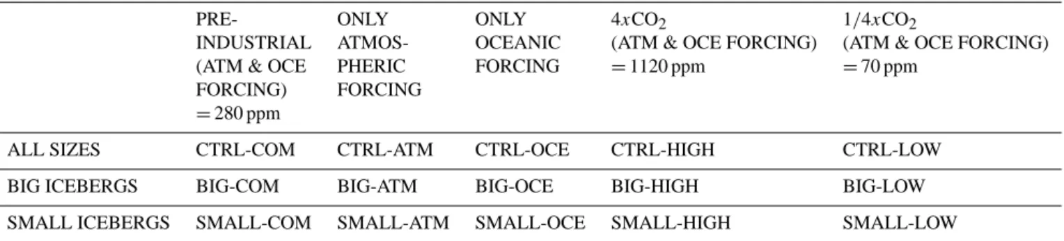
Table 1. Performed experiments.
PRE- ONLY ONLY 4xCO2 1/4xCO2
INDUSTRIAL ATMOS- OCEANIC (ATM & OCE FORCING) (ATM & OCE FORCING)
(ATM & OCE PHERIC FORCING =1120 ppm =70 ppm
FORCING) FORCING
=280 ppm
ALL SIZES CTRL-COM CTRL-ATM CTRL-OCE CTRL-HIGH CTRL-LOW
BIG ICEBERGS BIG-COM BIG-ATM BIG-OCE BIG-HIGH BIG-LOW
SMALL ICEBERGS SMALL-COM SMALL-ATM SMALL-OCE SMALL-HIGH SMALL-LOW
We will address these questions by presenting results from 15 different sensitivity experiments (Table 1) that differ in the applied forcing (atmospheric, oceanic, pre-industrial, warmer, colder climate) and the initial size distribution (CTRL (standard sizes), BIG, SMALL, Table 2) of the ice-bergs.
We will first introduce the model and the experimental set-up, then present the results and the discussion, followed by a conclusion section.
2 Methods
We use the earth system model of intermediate complex-ity iLOVECLIM (version 1.0) which is a code fork of the LOVECLIM climate model version 1.2 (Goosse et al., 2010). iLOVECLIM differs in the ice sheet module included (Roche et al., 2014) and the further developed iceberg mod-ule (Bügelmayer et al., 2015), but shares some physical cli-mate components (atmosphere, ocean and vegetation) with LOVECLIM.
2.1 Atmosphere–ocean–vegetation model
The iLOVECLIM climate model consists of the EC-Bilt atmospheric model (Opsteegh et al., 1998), a quasi-geostrophic, spectral model with a horizontal resolution of T21 (5.6◦ in latitude/longitude) and three vertical pressure levels (800, 500, 200 hPa). The atmospheric state (including e.g. temperature, humidity) is calculated every 4 h. Precip-itation depends on the available humidity in the lowermost atmospheric level and the total solid precipitation is given to the ice sheet model at the end of one model year, as are the monthly surface temperatures.
iLOVECLIM includes the sea-ice and ocean model CLIO, which is a three-dimensional ocean general circu-lation model (Deleersnijder and Campin, 1995; Deleer-snijder et al., 1997; Campin and Goosse, 1999) includ-ing a dynamic–thermodynamic sea-ice model (Fichefet and Morales Maqueda, 1997, 1999). Due to its free surface, the freshwater fluxes related to iceberg melting can be directly applied to the ocean’s surface. The horizontal resolution is
3◦×3◦in longitude and latitude and the ocean is vertically divided into 20 unevenly spaced layers. CLIO uses a realistic bathymetry. The oceanic variables (e.g. sea surface tempera-ture and salinity) are computed once a day.
The vegetation (type and cover) is calculated by the VE-CODE vegetation model (Brovkin et al., 1997), which runs on the same grid as ECBilt. VECODE accounts for fractional use of one grid cell because of the small spatial changes in vegetation. It simulates the dynamics of two plant functional types (trees and grass) as well as bare soil in response to the temperature and precipitation coming from ECBilt.
The Antarctic ice sheet is prescribed according to present-day conditions following the ETOPO1 topography (http: //www.ngdc.noaa.gov/mgg/global/global.html). Icebergs are parameterized in the form of homogenous uptake of latent heat around Antarctica, thereby cooling the ocean without al-tering the salinity. Ice shelf melting is computed according to the prevailing ocean temperatures. The Greenland ice sheet is actively simulated using the GRISLI ice sheet model.
2.2 GRISLI – ice sheet model
The ice sheet model included in iLOVECLIM is the Greno-ble model for Ice Shelves and Land Ice (GRISLI), which is a three-dimensional thermomechanical model that was first developed for the Antarctic (Ritz et al., 1997, 2001) and was further developed for the Northern Hemisphere (Peyaud et al., 2007). GRISLI consists of a Lambert azimuthal grid with a 40 × 40 km horizontal resolution. In the present study, it computes the evolution of the thickness and extension of the Greenland ice sheet (GrIS) only, as we exclude the South-ern Hemisphere grid. GRISLI distinguishes three types of ice flow: inland ice, ice streams and ice shelves. Calving takes place whenever the ice thickness at the border of the ice sheet is less than 150 m and the points upstream do not provide enough inflow of ice to maintain this thickness. After one model year, the total yearly amount of calving is given to the iceberg module where icebergs are generated daily, as described in detail in Sect. 2.3. The runoff of GRISLI is cal-culated at the end of the year by computing the difference between the ice sheet thickness at the beginning of the model year and the end of the year, and taking into account the mass
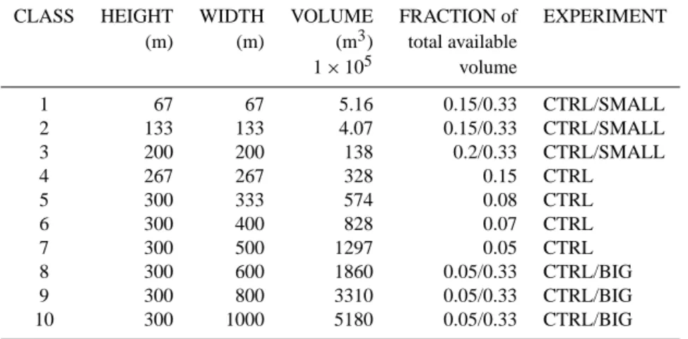
Table 2. Used initial iceberg classes.
CLASS HEIGHT WIDTH VOLUME FRACTION of EXPERIMENT
(m) (m) (m3) total available 1 × 10⁵ volume 1 67 67 5.16 0.15/0.33 CTRL/SMALL 2 133 133 4.07 0.15/0.33 CTRL/SMALL 3 200 200 138 0.2/0.33 CTRL/SMALL 4 267 267 328 0.15 CTRL 5 300 333 574 0.08 CTRL 6 300 400 828 0.07 CTRL 7 300 500 1297 0.05 CTRL 8 300 600 1860 0.05/0.33 CTRL/BIG 9 300 800 3310 0.05/0.33 CTRL/BIG 10 300 1000 5180 0.05/0.33 CTRL/BIG
loss due to calving. The runoff is then given to ECBilt where it is re-computed to fit its time step (4 h) and incorporated into the land routing system. GRISLI is run for one model year and then provides the runoff and calving, as well as the updated albedo and topography fields to the atmosphere– ocean–vegetation component. A more detailed explanation of the coupling between ECBilt, CLIO and the GRISLI ice sheet model is provided in Roche et al. (2014) and Bügel-mayer et al. (2015).
2.3 Iceberg module
As discussed in detail in Bügelmayer et al. (2015), the dynamic–thermodynamic iceberg module (Jongma et al., 2009; Wiersma and Jongma, 2010) included in iLOVECLIM is based on the iceberg-drift model of Smith and co-workers (Smith and Banke, 1983; Smith, 1993; Loset, 1993) and on the developments done by Bigg et al. (1996, 1997) and Glad-stone et al. (2001). According to the calving mass and loca-tions calculated by GRISLI over one model year, icebergs of up to ten size classes are generated. The provided ice mass is re-computed to fit the daily time step of the iceberg mod-ule, taking into account the seasonal calving cycle, with the maximum calving occurring from April to June and the min-imum occurring in late summer (Martin and Adcroft, 2010). The control size distribution of the icebergs is according to Bigg et al. (1996) and based on observations of Dowdeswell et al. (1992) that represent the Greenland present-day distri-bution (Table 2). It does not take into account huge tabular icebergs such as those calved from Antarctica, but is a valid representation for icebergs calving from the Greenland ice sheet. The thickness and width of the calving front as de-fined in GRISLI affect the amount of ice mass available to generate icebergs, but not the icebergs’ dimensions. Icebergs are moved by the Coriolis force, the air-, water-, and sea-ice drag, the horizontal pressure gradient force and the wave radiation force. The forcing fields are provided by ECBilt (winds) and CLIO (ocean currents) and are linearly
interlated from the surrounding grid corners to the icebergs’ po-sitions. The icebergs melt over time due to basal melt, lateral melt and wave erosion and may roll over as their length to height ratio changes. The heat needed to melt the icebergs is taken from the ocean layers corresponding to the icebergs’ depth and the freshwater fluxes are put into the ocean surface layer of the current grid cell. The refreezing of melted water and the break-up of icebergs is not included in the iceberg module.
2.4 Experimental set-up
We have performed 15 sensitivity experiments that dif-fer in the initial size distribution (CTRL/SMALL/BIG, Ta-ble 2), in the applied CO2forcing (pre-industrial = 280 ppm,
4xCO2=1120 ppm, 1/4xCO2=70 ppm) or in the forces
that move the icebergs (atmosphere and ocean). A summary of the experiments performed is given in Table 1. All runs were started from an equilibrated climate and Greenland ice sheet under pre-industrial conditions that have already been used in the study of Bügelmayer et al. (2015). The initial ice sheet thickness is about 1/3 bigger than the observed one. We consider this bias negligible for the present study be-cause we focus on differences between our sensitivity runs using the same initial state for all experiments. The differ-ences between the individual simulations are therefore inde-pendent of the initial conditions and only functions of the different forcing applied. The model runs were conducted for 200 model years (pre-industrial) and 1000 model years (4xCO2, 1/4xCO2), respectively. The last 100 years are
pre-sented in the results.
2.4.1 Iceberg dynamical forcing
To differentiate between the impact of the ocean and the at-mosphere, we separate the individual forcing terms of the
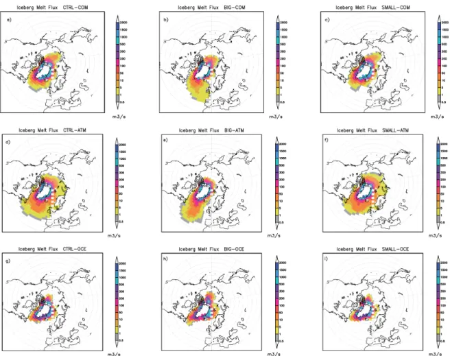
Figure 1. Iceberg melt flux (m3s−1); first row: the default set-up (icebergs are moved by both, atmospheric and oceanic forcing; CTRTL-, BIG-, SMALL-COM); second row: atmospheric forcing only (CTRL-, BIG-, SMALL-ATM); third row: oceanic forcing only (CTRL-, BIG-, SMALL-OCE).
equation of horizontal motion (Eq. 1) of an iceberg:
MdVi
dt = −Mfk · Vi+Fa+Fr+Fw+Fp+Fs, (1) with M being the mass of the iceberg, V its velocity, the first term (−Mfk · Vi) on the right side corresponding to the
Coriolis force, and the second and third being the air drag (Fa)and wave radiation force (Fr) and therefore depending
on the atmospheric winds; the last three terms represent the oceanic forcing, namely water drag (Fw), horizontal pressure
gradient (Fp) and sea-ice drag (Fs).
In the so-called “COM” experiments, the icebergs are moved according to Eq. (1), thus by the combined atmo-spheric and oceanic forcing. In the so-called “ATM” set-up, all the forcing terms corresponding to ocean currents are set to zero, thereby ensuring that the icebergs are only moved by the Coriolis and the atmospheric forcing. In the “OCE” set-up, on the contrary, the air drag and the wave radiation force are defined to be zero, thus only the Coriolis force and the ocean currents are acting on the icebergs.
The differentiation between atmospheric and oceanic forces was only made in the equation of motion of an iceberg.
The mass balance (Jongma et al., 2009), which depends on bottom and lateral melt (oceanic forcing) and the wave ero-sion (atmospheric forcing), is the same in all experiments. All the experiments are described in Table 1.
2.4.2 Iceberg initial size distribution
By altering the initial size distribution of the icebergs we are able to investigate the potential sensitivity of the atmo-sphere, ocean and ice sheet to iceberg sizes. In the CTRL ex-periments, depending on the available mass, icebergs of all 10 size classes can be generated (Bügelmayer et al., 2015). In the SMALL (BIG) experiments, the available mass is used to generate an equal amount of the three smallest (biggest) iceberg sizes (Table 2).
2.4.3 Radiative forcing
Using the three size distributions described in Sect. 2.4.2, we performed three sets of experiments. The first set was done under pre-industrial equilibrium conditions for 200 years. In the second one, a “high” experiment, we applied a CO2
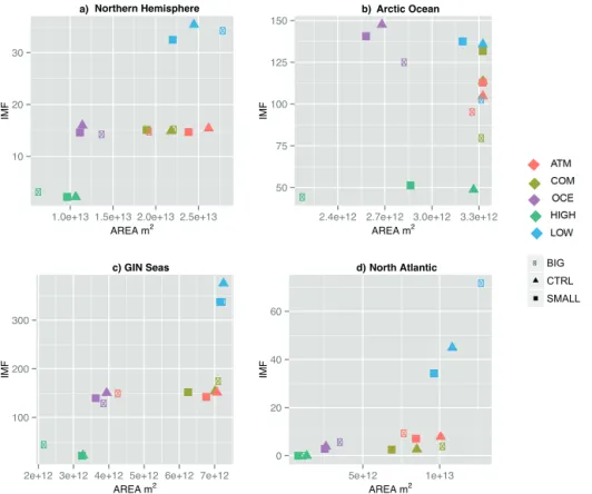
10 20 30
1.0e+13 1.5e+13 2.0e+13 2.5e+13 AREA m2 IMF a) Northern Hemisphere 50 75 100 125 150
2.4e+12 2.7e+12 3.0e+12 3.3e+12 AREA m2 IMF b) Arctic Ocean 100 200 300
2e+12 3e+12 4e+12 5e+12 6e+12 7e+12 AREA m2 IMF c) GIN Seas 0 20 40 60 5e+12 1e+13 AREA m2 IMF
d) North Atlantic BIG CTRL SMALL
Figure 2. Area (m2)vs. area weighted iceberg melt flux (m3s−1); the area is computed by taking into account all the grid cells that have at least 10 icebergs passing through per year (be aware that the area is 1013m2in a, 1012m2otherwise); (a) Northern Hemisphere: mean computed over 0–90◦N and 180◦W–180◦E, values of IMF: 0–40 m3s−1(area weighted IMF); (b) Arctic Ocean: 80–90◦N and 180◦W–180◦E, values of IMF: 60–140 m3s−1; (c) Greenland–Iceland–Norwegian (GIN) seas: 50–85◦N and 45◦W–15◦E, values of IMF: 40–240 m3s−1; (d) North Atlantic: 45–60◦N and 60–20◦W, values of IMF: 0–50 m3s−1.
concentration 4 times as strong as the pre-industrial value (1120 vs. 280 ppm CO2) and in the third, a “low”
exper-iment, only a quarter of the pre-industrial CO2
concentra-tion is used (70 vs. 280 ppm CO2). The “high” and “low”
experiments were conducted to analyse the effect of the size (CTRL/SMALL/BIG) distribution during periods of a strongly changing ice sheet under non-equilibrated condi-tions.
3 Results
3.1 Impact of dynamical forcing and initial iceberg size on the transport and lifetime of icebergs under pre-industrial conditions
3.1.1 The CTRL experiments
The distribution of the CTRL-COM’s iceberg melt flux dis-plays the general transport of icebergs of all size classes due to atmospheric and oceanic forces (Fig. 1a). We find that most iceberg melt flux is distributed along the eastern and western coasts of Greenland, displaying that the icebergs’ movement follows the oceanic currents. Furthermore, they
are moved southward along the North American coast and spread into the North Atlantic. In the Arctic, most icebergs are found close to Ellesmere Island, as indicated by the fresh-water flux, due to the calving sites in this region (not shown) and are then widely distributed by the Beaufort Gyre and the prevailing winds.
By applying only atmospheric forcing, we find that CTRL-ATM icebergs distribute their meltwater further into the North Atlantic and Arctic Ocean (Fig. 1d) than seen in CTRL-COM. After calving, they are quickly pushed away from the Greenland ice sheet margin. In CTRL-ATM fewer icebergs than in CTRL-COM melt along the coast of Green-land, highlighting the lack of ocean currents. Overall, the amount of iceberg melt flux released in CTRL-ATM (North-ern Hemisphere: 30 m3s−1; please note that this is an area
weighted mean) is of the same magnitude, but distributed over a broader area than in CTRL-COM (Fig. 2a). Yet, the lifetime of CTRL-ATM icebergs, that is the time (in months) it takes to completely melt the icebergs, is up to 1 year shorter than in CTRL-COM (Fig. 3) because they are transported faster away from the ice sheet and into warmer waters of the North Atlantic.
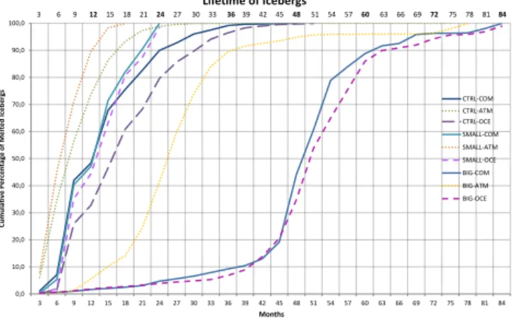
0,0 10,0 20,0 30,0 40,0 50,0 60,0 70,0 80,0 90,0 100,0 3 6 9 12 15 18 21 24 27 30 33 36 39 42 45 48 51 54 57 60 63 66 69 72 75 78 81 84 Cu m ul ati ve P er cen ta ge o f M el ted Ic ebe rg s Months Lifetime of Icebergs CTRL-COM CTRL-OCE SMALL-COM SMALL-ATM SMALL-OCE BIG-COM BIG-ATM BIG-OCE CTRL-ATM 3 6 9 12 15 18 21 24 27 30 33 36 39 42 45 48 51 54 57 60 63 66 69 72 75 78 81 84
Figure 3. Cumulative iceberg melt distribution normalized to 100 %
as a function of time (months); x axis corresponds to months, y axis to cumulative percentage.
The effect of the oceanic forcing is in strong contrast to the atmospheric one as it causes the CTRL-OCE icebergs to stay closer to the GrIS margin (Fig. 1g). The icebergs melt flux reflects the prevailing ocean currents, mainly the Beaufort Gyre, and the East Greenland and the Labrador cur-rents. Far fewer icebergs are moved from the ice sheet into the Greenland–Iceland–Norwegian (GIN) seas and the North Atlantic in CTRL-OCE compared to CTRL-COM (Fig. 1a, g) due to the lack of wind forcing, which is also reflected in the area that they cover (Fig. 2c, d). Also in the Arctic Ocean, the CTRL-OCE icebergs do not spread as much, but a slightly larger iceberg melt flux (IMF) is released because the icebergs are not transported southwards by the wind, but stay and melt there. Overall, the amount of freshwater flux is comparable to the CTRL-COM experiment, though over a much smaller area (CTRL-COM: 2.4 × 10¹³m2, CTRL-OCE: 1.2 × 10¹³m2, Fig. 2a) and over a longer time period.
The CTRL-OCE icebergs melt up to 4 months slower than CTRL-COM icebergs because they stay close to the GrIS margin and thus in colder water (Fig. 3).
3.1.2 The BIG experiments
The spatial distribution of the BIG-COM icebergs displays first, the effect of the Coriolis force since there is an east-ward movement in the North Atlantic (Fig. 1b). The Cori-olis force depends on the size and velocity of the icebergs and thus is acting more strongly on big icebergs than on small ones. Second, the area covered by BIG-COM icebergs is larger in the North Atlantic than in CTRL-COM (Fig. 2d). Over the Northern Hemisphere the area covered by more than 10 BIG-COM icebergs is only slightly bigger than the one of CTRL-COM (Fig. 2a), even though their lifetime is up to 3 years longer (Fig. 3). But in total there are fewer BIG ice-bergs generated than in the CTRL experiment because more mass is needed per berg (Table 2).
Applying only wind forcing to the BIG icebergs (BIG-ATM) transports fewer icebergs into the North Atlantic and especially the GIN seas (Fig. 1e), where they cover about half the area of BIG-COM (4 × 10¹²m2 compared to 7 × 10¹²m2), but release the same amount of freshwater (150 m3s−1, Fig. 2c). The strong southward component of the wind keeps the icebergs from drifting further into the GIN seas. Similar to the CTRL experiment, the BIG-ATM icebergs melt up to 2 years faster than the ones of BIG-COM or BIG-OCE (Fig. 3).
The impact of oceanic forcing on the iceberg melt flux is simulated in BIG-OCE. Since the big icebergs melt slowly, they are transported further south than CTRL-OCE icebergs (Fig. 1h). In the GIN seas the BIG-OCE icebergs are spread from the coast and cover almost the same area as the BIG-ATM (Fig. 2c). In the Arctic Ocean the BIG-OCE icebergs release a higher averaged melt flux than COM and BIG-ATM (125 m3s−1 compared to 75 and 95 m3s−1,
respec-tively; Fig. 2b), but over a smaller area. This is because of the missing wind forcing which prevents the icebergs from being distributed out of the Arctic Ocean. Instead the icebergs are stuck close to their calving sites. The higher IMF in BIG-OCE does not strongly impact the Arctic climate because of the prevailing cold conditions. Thus, more IMF, which is re-leased to the ocean surface layer at 0◦C and consequently cools and freshens it, does not cause noticeable changes. The area covered by BIG icebergs over the Northern Hemisphere is clearly bigger than SMALL-, or CTRL-OCE (Fig. 2a) be-cause of their lifetime, which is about 2 years longer com-pared to CTRL-OCE (Fig. 3).
3.1.3 The SMALL experiments
Generating only SMALL-COM icebergs results in a similar iceberg melt flux distribution as in CTRL-COM (Fig. 1c), but less widespread. The amount of freshwater that is released by SMALL-COM icebergs is almost the same over the Northern Hemisphere as CTRL-COM, but over a smaller area (Fig. 2a) because all the SMALL-COM icebergs are melted within 2 years, compared to 3 years in CTRL-COM (Fig. 3).
In the icebergs’ distribution of the SMALL-ATM model runs (Fig. 1f), it is clearly visible that the light, small ice-bergs are easily pushed away from their calving sites by the atmospheric forcing, but as in the COM experiments, over a smaller area because they melt faster. In the North Atlantic, the general pattern is directed westward, in contrast to BIG-ATM icebergs that are strongly influenced by the Coriolis force.
The widespread meltwater distribution of SMALL-ATM is in strong contrast to the one of SMALL-OCE (Fig. 1i). The oceanic forcing restricts the icebergs’ transport to the shore and due to their smaller size SMALL-OCE icebergs melt be-fore being distributed as far as CTRL-OCE and especially BIG-OCE (Fig. 2a).
In short, the impact of the forcing fields is clearly seen in the icebergs’ meltwater distribution and especially lifetime since 90 % of all the atmospheric forced icebergs (SMALL-, BIG-, and CTRL-ATM) melt up to 2 years faster compared to the oceanic forced icebergs and compared to the icebergs of the SMALL-, BIG-, and CTRL-COM set-up.
3.2 Impact of dynamical forcing and initial iceberg size on pre-industrial climate
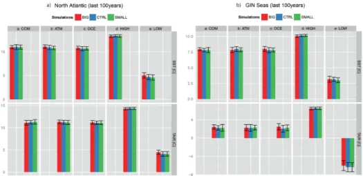
The resulting sea surface and air temperatures (SST, TAIR) are comparable between the CTRL-COM, -ATM, and -OCE experiments (Fig. 4a, b), despite the different spatial distri-bution of the iceberg melt flux. The biggest spread in IMF is found in the Arctic Ocean (BIG-COM: 75 m3s−1, CTRL-OCE: 150 m3s−1, Fig. 2c), but these differences do not result
in an altered climate state due to the prevailing cold condi-tions that are less sensitive to the freshening and cooling ef-fect of icebergs (not shown). Also in the GIN seas and North Atlantic, the difference in SST and TAIR between the exper-iments does not significantly differ from internal variability (Fig. 4). In all the pre-industrial experiments, we find that the differences in air and ocean temperature between the CTRL and the BIG, SMALL experiments do not significantly ex-ceed the internal variability of the CTRL experiment. This is also the case for sensitive areas such as the GIN Seas or the North Atlantic, due to the located convection sites there. Therefore, the impact of the dynamical forcing and initial iceberg size is smaller than natural climate variability, which is also reflected in the deep ocean circulation (not shown). This indicates that since the amount of freshwater released is comparable in the model runs, the exact location of the re-lease does not have a strong impact on the prevailing climate conditions or the ocean circulation. Furthermore, the shorter lifetime of the atmospheric driven icebergs does not cause differences in the resulting climate and the GrIS because the calving flux provided by GRISLI is almost constant over the years and comparable in all the pre-industrial experiments. Therefore, the same amount of freshwater is supplied to the ocean. Under pre-industrial equilibrium conditions the atmo-spheric and oceanic forcing do transport the icebergs differ-ently, but the resulting spatial patterns of the iceberg melt flux cause only local differences in the Greenland ice sheet volume (Table 3) that are within the internal variability of the ice sheet.
3.3 Impact of initial iceberg size under a changing climate
To have more confidence in using the present-day iceberg distribution also for simulations of past and future climates, we conducted two more sets of experiments with enhanced or reduced radiative forcing to obtain warmer and colder climate states. This change in radiative forcing was ap-plied through adjustment of the atmospheric CO2
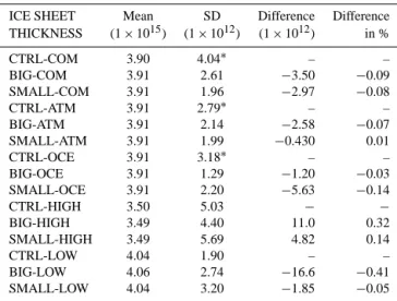
concen-Table 3. Ice sheet volume (m3): mean and standard deviation of the last 100 years; the∗corresponds to the CTRL SD that was com-puted over the last 200 years to have a more representative range of internal variability as a reference; difference between the ice sheet volume of the CTRL experiment and the BIG/SMALL experiments in absolute numbers, if the value is above 2 · SD of the CTRL exper-iments (∗), then the difference is significantly different from internal variability (none of the experiments); % diff = difference between the ice sheet volume of the CTRL experiment and the BIG/SMALL experiments in percent.
ICE SHEET Mean SD Difference Difference THICKNESS (1 × 10¹⁵) (1 × 10¹²) (1 × 10¹²) in % CTRL-COM 3.90 4.04∗ – – BIG-COM 3.91 2.61 −3.50 −0.09 SMALL-COM 3.91 1.96 −2.97 −0.08 CTRL-ATM 3.91 2.79∗ – – BIG-ATM 3.91 2.14 −2.58 −0.07 SMALL-ATM 3.91 1.99 −0.430 0.01 CTRL-OCE 3.91 3.18∗ – – BIG-OCE 3.91 1.29 −1.20 −0.03 SMALL-OCE 3.91 2.20 −5.63 −0.14 CTRL-HIGH 3.50 5.03 − − BIG-HIGH 3.49 4.40 11.0 0.32 SMALL-HIGH 3.49 5.69 4.82 0.14 CTRL-LOW 4.04 1.90 – – BIG-LOW 4.06 2.74 −16.6 −0.41 SMALL-LOW 4.04 3.20 −1.85 −0.05
tration in two experiments, the so-called HIGH = 4xCO2
(1120 ppm) and LOW = 1/4xCO2 (70 ppm), with a
dura-tion of 1000 years. For each of these settings, we performed experiments with CTRL, BIG and SMALL icebergs. The HIGH experiments resulted in an up to 4◦C warmer global mean temperature and caused the Greenland ice sheet to lose 10 % of its volume, whereas the LOW experiments caused the mean global temperatures to decrease about 4◦C and an
increase of the Greenland ice sheet volume of up to 4 %, compared to the pre-industrial ice sheet volume (Table 3).
3.3.1 Experiments with high radiative forcing
The impact of the enhanced radiative forcing on the Green-land ice sheet is displayed in Fig. 5, where the resulting CTRL-HIGH ice sheet extensions and thickness are shown (Fig. 5b).
As the ice sheet is shrinking and retreating from the coast (Fig. 5b), the calving flux from the GrIS is decay-ing (0.003 Sv vs. 0.02 Sv in the CTRL-COM), which is re-flected in the IMF and the area that they cover (Fig. 2). The strong retreat of the ice sheet in southern Greenland has a direct impact on the iceberg melt flux. The released iceberg melt flux in the GIN seas is in the range of 20 (SMALL-, CTRL-HIGH) to 50 m3s−1 (BIG-HIGH, Fig. 2c), com-pared to 150 m3s−1in the CTRL-COM. Moreover, there are hardly any icebergs entering the North Atlantic, independent of the used size distribution (Fig. 2d). In the Arctic Ocean
Figure 4. Mean + standard deviation of the last 100 years of the performed experiments: sea surface temperature (SST,◦C) and air tem-perature (TAIR,◦C); red = BIG icebergs, blue = CTRL, green = SMALL icebergs; (a) North Atlantic: mean computed over: 45–60◦N and 60–20◦W; (b) Greenland–Iceland–Norwegian (GIN) seas: 50–85◦N and 45◦W–15◦E.
the HIGH experiments result in a bigger spread between the CTRL, BIG and SMALL runs than any other performed set-up (Fig. 2b). The BIG-HIGH icebergs cover the smallest area because of the decreased calving flux far fewer BIG ones are generated. Furthermore, there are still SMALL icebergs, but due to their size and the warmer conditions they melt faster than seen in the SMALL experiments performed under pre-industrial conditions. The CTRL-HIGH experiment covers a slightly smaller area than the CTRL-COM,-OCE or -ATM, but much bigger than BIG-, and SMALL-HIGH (Fig. 2b). This is because the different iceberg sizes allow for the pro-duction of a higher number of icebergs than in BIG and the existence of icebergs bigger than size 3 (as in SMALL) al-lows for a longer lifetime.
Although the size of the icebergs generated varies from the beginning, the resulting climate conditions, such as sea sur-face or air temperatures, do not vary at the end of the 1000-year period between the SMALL-, BIG-, and CTRL-HIGH experiments (Fig. 4a, b), nor does the GrIS (Table 3). Dur-ing periods of strong background changes, different iceberg distributions do not result in different climate states. This in-dicates that the applied forcing has a stronger impact than local differences due to the chosen iceberg size.
3.3.2 Experiments with low radiative forcing
In contrast to the experiments with high radiative forcing, the low radiative forcing causes up to 4◦C lower global
mean temperatures and consequently the ice sheet’s volume is thickening and extending further down to the coastline (Fig. 5c), especially along the western margin and in south-ern Greenland. Similar to the other experiments performed, the impact of different initial size distributions of the icebergs is negligible on the resulting climate and ice sheet volume (Table 3).
Due to the increased ice sheet thickness, more calving flux is released (0.05 Sv in CTRL-LOW compared to 0.02 Sv in CTRL-COM) and so the iceberg melt flux increases to
∼40 m3s−1 over the Northern Hemisphere, compared to 15 m3s−1in the pre-industrial experiments. The increase is seen almost everywhere around Greenland (Fig. 2), except in the Arctic Ocean. In the Arctic Ocean the released IMF is in the same range as in the experiments performed under pre-industrial conditions because the ice sheet’s thickness and consequently the calving sites in North Greenland are not strongly altered by the colder climate (Fig. 5c). In the North Atlantic the released iceberg melt flux displays a big spread between the experiments with the BIG-LOW icebergs being spread the furthest and releasing the most IMF (80 m3s−1in BIG-LOW vs. 45 m3s−1in CTRL-LOW; Fig. 2d). Since the cold conditions prevent the BIG-LOW icebergs from melt-ing quickly, almost all of them are transported into the North Atlantic where they finally melt. This is also partly the case for the CTRL-LOW icebergs, thereby resulting in a higher iceberg melt flux than the SMALL-LOW (Fig. 2d). Indepen-dent of the chosen size distribution, the resulting tempera-tures are about 5◦C lower than during pre-industrial condi-tions in the North Atlantic and the GIN seas (Fig. 4), display-ing the strong CO2forcing.
During a strongly changing climate, the initial size dis-tribution does not alter the climate response (temperatures, ocean circulation) more strongly than internal variability. The BIG-LOW set-up causes a slightly larger mean ice sheet volume at the end of the 1000 years (Table 3), which indi-cates that the extreme case of BIG icebergs impacts the re-sulting ice sheet thickness, even though the climate condi-tions are similar to the CTRL- and SMALL-LOW runs.
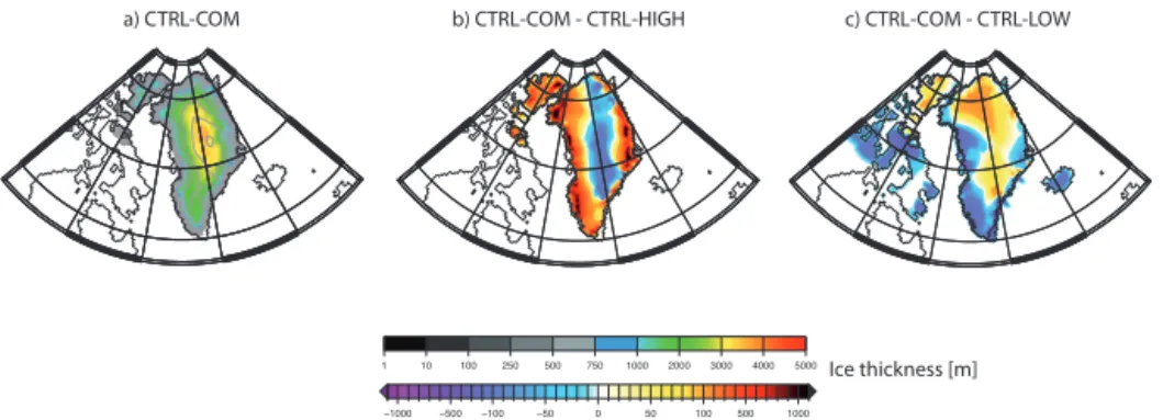
1 10 100 250 500 750 1000 2000 3000 4000 5000
−1000 −500 −100 −50 0 50 100 500 1000
a) CTRL-COM b) CTRL-COM - CTRL-HIGH c) CTRL-COM - CTRL-LOW
Ice thickness [m]
Figure 5. (a) CTRL-COM ice sheet thickness at the end of the experiments (m); (b) difference in ice sheet thickness at the end of the model
runs CTRL-COM minus CTRL-HIGH; (c) difference in ice sheet thickness at the end of the model runs CTRL-COM minus CTRL-LOW.
4 Discussion
By testing the impact of the atmospheric versus the oceanic forcing on the lifetime and motion of icebergs, we find that the atmospheric forcing causes the icebergs to travel further away from their calving sites and into the North Atlantic, whereas the ocean currents lead to iceberg tracks closer to shore. It is difficult to compare our results to previous stud-ies, since the studies that investigated the impact of the back-ground forcing (Smith, 1993; Keghouche et al., 2002) fo-cused on observations of single icebergs and the ability of models reproducing their specific tracks. Bigg et al. (1997) noted that the modelling of specific iceberg tracks is very un-likely to be successful and it is important to notice that we do not expect our model to resolve single tracks due to its coarse resolution, but to reflect the widespread effect of icebergs on climate.
In our model, the impact of icebergs on climate does not strongly depend on the two types of forcing (atmospheric and oceanic), yet their lifetime is shortened by up to 2 years when they are transported by atmospheric forces only. Bigg et al. (1997) showed that about 80 % of the small icebergs of up to 200 m diameter (size class 1 to 3, Table 2) melt within the first year, which is higher than in our SMALL-COM set-up where about 60 % are melted. Also Venkatesh and El-Tahan (1988) conducted a study to investigate the impact of modelling complete deterioration of icebergs on the predic-tion of their tracks. In their study they showed that most of the icebergs corresponding to size classes 1 to 3 used in this study, disappear within 3 to 22 months, consistent with our results. The maximum lifetime of the BIG icebergs is found to be almost 7 years, which is slightly longer than modelled by Bigg et al. (1997). This discrepancy can be due to the pre-industrial climate conditions used in our study that are slightly colder than the present-day conditions applied by Bigg et al. (1997).
To better understand the response of the modelled climate to the initial size distribution, we performed different sensi-tivity experiments. First, using pre-industrial conditions we find that independent of the forcing, SMALL icebergs
re-lease less freshwater and spread over a smaller area than BIG and CTRL icebergs. In the North Atlantic the impact of the Coriolis force is especially pronounced in the BIG-ATM and BIG-COM runs, confirming the findings of Roberts et al. (2014). In their study they noted that BIG icebergs travel further south than small icebergs due to the stronger impact of the Coriolis force. Even though the SMALL ice-bergs cause locally different ocean and atmospheric condi-tions than the BIG icebergs, the overall effect on climate and on the Greenland ice sheet is within the natural climate vari-ability.
Second, we repeated the experiments under a strongly in-creased and dein-creased radiative forcing for 1000 years. Dur-ing this time, scale changes in the Southern Ocean can im-pact the Northern Hemisphere. Jongma et al. (2009) showed that including active icebergs increases the net production of Antarctic Bottom Water by 10 % under pre-industrial condi-tions. We do neglect this direct effect of icebergs here since icebergs and Antarctic ice sheet runoff are computed using parameterizations that depend on the prevailing climate con-ditions. Concerning the icebergs released from Greenland, we do not expect that the size of the icebergs will have an im-pact on the Southern Hemisphere through altered ocean cir-culation because the Atlantic Meridional Overturning Circu-lation is comparable within all the experiments (not shown). Thus, the uncertainty introduced by not actively coupling the Antarctic ice sheet is comparable in all the radiative forcing experiments.
There might be different reasons why the climate condi-tions and the GrIS are not strongly affected by the initial size distribution during strong radiative background conditions. One reason could be that the ice sheet and the climate model are too insensitive to the experienced changes as they have a relatively coarse resolution. Therefore, it would be interest-ing to repeat this study with a finer model grid. Another rea-son might be that in the experiments where really strong forc-ing was applied (HIGH = 1120 ppm CO2, LOW = 70 ppm
CO2), the feedbacks related to calving have a smaller signal
5 Conclusions
Within a fully coupled climate–ice sheet–iceberg model set-up, we have performed sensitivity experiments to investigate the effect of the forcing fields such as winds and ocean cur-rents, as well as the prescribed initial size distribution, on the icebergs and the climate.
We find that, under pre-industrial conditions, the wind forcing pushes the icebergs further away from their calving sites and further into the North Atlantic, whereas the ocean currents transport the icebergs close to Greenland and south-ward along the North American coast. The combined effect of the forces (control set-up) displays a lesser spread iceberg distribution in the Arctic Ocean and into the North Atlantic than the purely atmospheric driven icebergs due to the re-strictive effects of the oceanic forcing. The spread of icebergs depends on both the forcing fields and the iceberg size with the CTRL icebergs being transported the furthest, followed by the BIG icebergs. The amount of released iceberg melt flux is comparable in all the experiments, though locally dif-ferent. In our model set-up, the biggest impact of the applied forcing (atmospheric or oceanic) is on the icebergs’ lifetime, which is up to 2 years shorter if the icebergs are only trans-ported by winds.
In the presented model framework, the implementation of icebergs of different size classes under equilibrated pre-industrial conditions reveals that there are local differences in the released freshwater flux. However, these differences do not cause significant changes in the resulting Greenland ice sheet volume and climate conditions.
When repeating the experiments with different size distri-butions with strong radiative cooling or warming (1120 or 70 ppm CO2, 1000 model years), the response of the climate
and the ice sheet volume do not differ strongly within the experiments.
Even though the iceberg and freshwater distribution dif-fer between the conducted experiments (all size classes, only SMALL, less than 200 m width, and only BIG icebergs, 600– 1000 m width, respectively), their impact on the Northern Hemispheric climate does not differ significantly from in-ternal variability. We can therefore conclude that for the re-sulting climate and ice sheet, small spatial differences be-tween the runs do not have a strong impact as long as there is a widespread impact of icebergs (cooling and freshening) around Greenland. Furthermore, our results show that the re-sponse of the climate to the applied radiative forcing is much stronger than its response to the chosen initial size distribu-tion of the icebergs.
Code availability
The iLOVECLIM source code is based on the LOVE-CLIM model version 1.2 whose code is accessible at http:// www.elic.ucl.ac.be/modx/elic/index.php?id=289. The devel-opments on the iLOVECLIM source code are hosted at https:
//forge.ipsl.jussieu.fr/ludus, but are not publicly available due to copyright restrictions. Access can be granted on demand by request to D. M. Roche ([email protected]). The specific experimental set-up used for this study is available at https://forge.ipsl.jussieu.fr/ludus.
The Supplement related to this article is available online at doi:10.5194/gmd-8-2139-2015-supplement.
Acknowledgements. M. Bügelmayer is supported by NWO through
the VIDI/AC2ME project no. 864.09.013. D. M. Roche is sup-ported by NWO through the VIDI/AC2ME project no. 864.09.013 and by CNRS-INSU. The authors wish to thank Catherine Ritz for the use of the GRISLI ice sheet model and all the anony-mous reviewers for providing valuable comments. Institut Pierre Simon Laplace is gratefully acknowledged for hosting the
iLOVECLIM model code under the LUDUS framework project (https://forge.ipsl.jussieu.fr/ludus). This is NWO/AC2ME contri-bution number 08.
Edited by: R. Marsh
References
Álvarez-Solas, J., Montoya, M., Ritz, C., Ramstein, G., Charbit, S., Dumas, C., Nisancioglu, K., Dokken, T., and Ganopolski, A.: Heinrich event 1: an example of dynamical ice-sheet reaction to oceanic changes, Clim. Past, 7, 1297–1306, doi:10.5194/cp-7-1297-2011, 2011.
Andrews, J. T.: Abrupt changes (Heinrich events) in late Qua-ternary North Atlantic marine environments: a history and review of data and concepts, J. Quaternary Sci., 13, 3– 16, doi:10.1002/(SICI)1099-1417(199801/02)13:1<3::AID-JQS361>3.0.CO;2-0, 1998.
Bigg, G. R., Wadley, M. R., Stevens, D. P., and Johnson, J. V.: Pre-diction of iceberg trajectories for the North Atlantic and Arctic Oceans, Geophys. Res. Lett., 23, 3587–3590, 1996.
Bigg, G. R., Wadley, M. R., Stevens, D. P., and Johnson, J. V.: Mod-elling the dynamics and thermodynamics of icebergs, Cold Reg. Sci. Technol., 26, 113–135, doi:10.1016/S0165-232X(97)00012-8, 1997.
Broecker, W. S., Bond, G., and McManus, J.: Heinrich events: Trig-gers of ocean circulation change?, in: Ice in the climate system: NATO ASI Series, edited by: Peltier, W. R., Vol. 12, Springer-Verlag, Berlin, 161–166, doi:10.1007/978-3-642-85016-5_10, 1993.
Brovkin, V., Ganopolski, A., and Svirezhev, Y.: A continuous climate-vegetation classification for use in climate-biosphere studies, Ecol. Model., 101, 251–261, 1997.
Bügelmayer, M., Roche, D. M., and Renssen, H.: How do icebergs affect the Greenland ice sheet under pre-industrial conditions? – a model study with a fully coupled ice-sheet-climate model, The Cryosphere, 9, 821–835, doi:10.5194/tc-9-821-2015, 2015.
Campin, J. M. and Goosse, H.: A parameterization of density driven downsloping flow for coarse resolution model in z-coordinate, Tellus, 51A, 412–430, 1999.
Death, R., Siegert, M. J., Bigg, G. R. and Wadley, M. R.: Modelling iceberg trajectories, sedimentation rates and melt-water input to the ocean from the Eurasian Ice Sheet at the Last Glacial Maximum, Palaeogeogr. Palaeocl., 236, 135–150, doi:10.1016/j.palaeo.2005.11.040, 2005.
Deleersnijder, E., Beckers, J.-M., Campin, J.-M., El Mohajir, M., Fichefet, T., and Luyten, P.: Some mathematical problems asso-ciated with the development and use of marine models, in: The mathematics of model for climatology and environment, edited by: Diaz, J. I., NATO ASI Series, Vol. I 48, Springer-Verlag, 39– 86, 1997.
Deleersnijder, E. and Campin, J.-M.: On the computation of the barotropic mode of a free-surface world ocean model, Ann. Geo-phys., 13, 675–688, doi:10.1007/s00585-995-0675-x, 1995. Dowdeswell, J. A., Whittington, R. J., and Hodgkins, R.: The Sizes,
Frequencies, and Freeboards of East Greenland Icebergs Ob-served Using Ship Radar and Sextant, J. Geophys. Res., 97, 3515–3528, 1992.
Fichefet, T. and Morales Maqueda, M. A.: Sensitivity of a global sea ice model to the treatment of ice thermodynamics and dynamics, J. Geophys. Res., 102, 12609–12646, 1997.
Fichefet, T. and Morales Maqueda, M. A.: Modelling the influence of snow accumulation and snow-ice formation on the seasonal cycle of the Antarctic sea-ice cover, Clim. Dynam., 15, 251–268, 1999.
Gherardi, J., Labeyrie, L., McManus, J., Francois, R., Skinner, L., and Cortijo, E.: Evidence from the Northeastern Atlantic basin for variability in the rate of the meridional overturning circula-tion through the last deglaciacircula-tion, Earth Planet. Sc. Lett., 240, 710–723, doi:10.1016/j.epsl.2005.09.061, 2005.
Gladstone, R. M., Bigg, G. R., and Nicholls, K. W.: Iceberg trajec-tory modeling and meltwater injection in the Southern Ocean, J. Geophys. Res., 106, 19903–19915, doi:10.1029/2000JC000347, 2001.
Goosse, H., Brovkin, V., Fichefet, T., Haarsma, R., Huybrechts, P., Jongma, J., Mouchet, A., Selten, F., Barriat, P.-Y., Campin, J.-M., Deleersnijder, E., Driesschaert, E., Goelzer, H., Janssens, I., Loutre, M.-F., Morales Maqueda, M. A., Opsteegh, T., Mathieu, P.-P., Munhoven, G., Pettersson, E. J., Renssen, H., Roche, D. M., Schaeffer, M., Tartinville, B., Timmermann, A., and Weber, S. L.: Description of the Earth system model of intermediate complex-ity LOVECLIM version 1.2, Geosci. Model Dev., 3, 603–633, doi:10.5194/gmd-3-603-2010, 2010.
Green, C. L., Green, J. A. M., and Bigg, G. R.: Simulating the im-pact of freshwater inputs and deep-draft icebergs formed during a MIS 6 Barents Ice Sheet collapse, Paleoceanography, 26, 1–16, doi:10.1029/2010PA002088, 2011.
Hemming, S. R.: Heinrich Events: Massive Late Pleistocene Detri-tus Layers of the North Atlantic and their global climate imprint, Rev. Geophys., 42, 1–43, doi:10.1029/2003RG000128, 2004. Hooke, R. L.: Principles of Glacier Mechanics, 2nd Edn.,
Cam-bridge University Press, 2005.
Hulbe, C. L., MacAyeal, D. R., Denton, G. H., Kleman, J., and Vowell, T. V.: Catastrophic ice shelf breakup as the source of Heinrich event icebergs, Paleoceanography, 19, 1–16, doi:10.1029/2003PA000890, 2004.
Jongma, J. I., Driesschaert, E., Fichefet, T., Goosse, H., and Renssen, H.: The effect of dynamic–thermodynamic icebergs on the Southern Ocean climate in a three-dimensional model, Ocean Model., 26, 104–113, doi:10.1016/j.ocemod.2008.09.007, 2009. Jongma, J. I., Renssen, H., and Roche, D. M.: Simulating Heinrich event 1 with interactive icebergs, Clim. Dynam., 40, 1373–1385, doi:10.1007/s00382-012-1421-1, 2013.
Kageyama, M., Paul, A., Roche, D. M., and Van Meerbeeck, C. J.: Modelling glacial climatic millennial-scale variabil-ity related to changes in the Atlantic meridional overturning circulation: a review, Quaternary Sci. Rev., 29, 2931–2956, doi:10.1016/j.quascirev.2010.05.029, 2010.
Keghouche, I., Bertino, L., and Lisæter, K. A.: Parameterization of an Iceberg Drift Model in the Barents Sea, J. Atmos. Ocean. Tech., 26, 2216–2227, doi:10.1175/2009JTECHO678.1, 2009. Levine, R. C. and Bigg, G. R.: Sensitivity of the glacial ocean to
Heinrich events from different iceberg sources, as modeled by a coupled atmosphere-iceberg-ocean model, Paleoceanography, 23, 1–16, doi:10.1029/2008PA001613, 2008.
Loset, S.: Thermal-Energy Conservation in Icebergs and Track-ing by Temperature, J. Geophys. Res.-Oceans, 98, 10001–10012, 1993.
MacAyeal, D.: Binge/purge oscillations of the Laurentide ice sheet as a cause of the North Atlantic’s Heinrich events, Paleoceanogr. Palaeocl., 8, 775–784, 1993.
Marcott, S. A, Clark, P. U., Padman, L., Klinkhammer, G. P., Springer, S. R., Liu, Z., Otto-Bliesner, B. L., Carlson, A. E., Ungerer, A., Padman, J., He, F., Cheng, J., and Schmittner, A.: Ice-shelf collapse from subsurface warming as a trigger for Heinrich events, P. Natl. Acad. Sci. USA, 108, 13415–13419, doi:10.1073/pnas.1104772108, 2011.
Martin, T. and Adcroft, A.: Parameterizing the fresh-water flux from land ice to ocean with interactive icebergs in a coupled climate model, Ocean Model., 34, 111–124, doi:10.1016/j.ocemod.2010.05.001, 2010.
McManus, J. F., Francois, R., Gherardi, J.-M., Keigwin, L. D., and Brown-Leger, S.: Collapse and rapid resumption of Atlantic meridional circulation linked to deglacial climate changes, Na-ture, 428, 834–837, doi:10.1038/nature02494, 2004.
Opsteegh, J. D., Haarsma, R. J., Selten, F. M., and Kattenberg, A.: ECBilt: A dynamic alternative to mixed boundary conditions in ocean models, Tellus A, 50, 348–367, 1998.
Peyaud, V., Ritz, C., and Krinner, G.: Modelling the Early We-ichselian Eurasian Ice Sheets: role of ice shelves and influence of ice-dammed lakes, Clim. Past, 3, 375–386, doi:10.5194/cp-3-375-2007, 2007.
Rignot, E., Jacobs, S., Mouginot, J., and Scheuchl, B.: Ice-shelf melting around Antarctica, Science, 341, 266–270, doi:10.1126/science.1235798, 2013.
Ritz, C., Fabre, A., and Letréguilly, A.: Sensitivity of a Green-land ice sheet model to ice flow and ablation parameters: con-sequences for the evolution through the last climatic cycle, Clim. Dynam., 13, 11–23, doi:10.1007/s003820050149, 1997. Ritz, C., Rommelaere, V., and Dumas, C.: Modeling the evolution
of Antarctic ice sheet over the last 420,000 years: Implications for altitude changes in the Vostok region, J. Geophys. Res., 106, 31943–31964, doi:10.1029/2001JD900232, 2001.
Roberts, W. H. G., Valdes, P. J., and Payne, A. J.: A new constraint on the size of Heinrich Events from an iceberg/sediment model,
Earth Planet. Sc. Lett., 386, 1–9, doi:10.1016/j.epsl.2013.10.020, 2014.
Roche, D. M., Dumas, C., Bügelmayer, M., Charbit, S., and Ritz, C.: Adding a dynamical cryosphere to iLOVECLIM (version 1.0): coupling with the GRISLI ice-sheet model, Geosci. Model Dev., 7, 1377–1394, doi:10.5194/gmd-7-1377-2014, 2014.
Smith, K. L.: Free-drifting icebergs in the Southern Ocean:
An overview, Deep-Sea Res. Pt. II, 58, 1277–1284,
doi:10.1016/j.dsr2.2010.11.003, 2011.
Smith, S. D.: Hindcasting iceberg drift using current profiles and winds, Cold Reg. Sci. Technol., 22, 33–45, doi:10.1016/0165-232X(93)90044-9, 1993.
Smith, S. D. and Banke, E. G.: The influence of winds, currents and towing forces on the drift of icebergs, Cold Reg. Sci. Technol., 6, 241–255, 1983.
Tournadre, J., Girard-Ardhuin, F., and Legrésy, B.: Antarctic ice-bergs distributions, 2002–2010, J. Geophys. Res., 117, C05004, doi:10.1029/2011JC007441, 2012.
Venkatesh, S. and El-Tahan, M.: Iceberg life expectancies in the Grand Banks and Labrador Sea, Cold Reg. Sci. Technol., 15, 1– 11, 1988.
Wiersma, A. P. and Jongma, J. I.: A role for icebergs in the 8.2 ka climate event, Clim. Dynam., 35, 535–549, doi:10.1007/s00382-009-0645-1, 2010.