HAL Id: hal-01460706
https://hal.archives-ouvertes.fr/hal-01460706v2
Submitted on 5 Apr 2017
HAL is a multi-disciplinary open access
archive for the deposit and dissemination of
sci-entific research documents, whether they are
pub-lished or not. The documents may come from
teaching and research institutions in France or
abroad, or from public or private research centers.
L’archive ouverte pluridisciplinaire HAL, est
destinée au dépôt et à la diffusion de documents
scientifiques de niveau recherche, publiés ou non,
émanant des établissements d’enseignement et de
recherche français ou étrangers, des laboratoires
publics ou privés.
Distributed under a Creative Commons Attribution| 4.0 International License
Martin Mihelich, Davide Faranda, Didier Paillard, Bérengère Dubrulle
To cite this version:
Martin Mihelich, Davide Faranda, Didier Paillard, Bérengère Dubrulle. Is Turbulence a State of
Maximal Dissipation?. Entropy, MDPI, 2017, �10.3390/e19040154�. �hal-01460706v2�
Is Turbulence a State of Maximum Energy
Dissipation?
Martin Mihelich1,†, Davide Faranda2, Didier Paillard2and Bérengère Dubrulle1,*
1 SPEC, CEA, CNRS, Université Paris-Saclay, CEA Saclay 91191 Gif sur Yvette cedex, France 2 LSCE-IPSL, CEA Saclay l’Orme des Merisiers, CNRS UMR 8212 CEA-CNRS-UVSQ, Université
Paris-Saclay, 91191 Gif-sur-Yvette, France
* Correspondence: berengere.dubrulle@cea.fr; Tel.: +33-169 087 247 † Current address: ma.mihelich@gmail.com
Academic Editor: name
Version March 22, 2017 submitted to Entropy
Abstract: Turbulent flows are known to enhance turbulent transport. It has then even been 1
suggested that turbulence is a state of maximum energy dissipation. In this paper, we re-examine 2
critically this suggestion at the light of several recent works around the Maximum Entropy 3
Production principle (MEP) that has been used in several out-of-equilibrium systems. We provide 4
a set of 4 different optimization principles, based on maximization of energy dissipation, entropy 5
production, Kolmogorov-Sinai entropy and minimization of mixing time, and study the connection 6
between these principles using simple out-of-equilibrium models describing mixing of a scalar 7
quantity. We find that there is a chained-relationship between most probable stationary states of 8
the system, and their ability to obey one of the 4 principle. This provides an empirical justification 9
of the Maximum Entropy Production principle in this class of systems, including some turbulent 10
flows, for special boundary conditions. Otherwise, we claim that the minimization of the mixing 11
time would be a more appropriate principle. We stress that this principle might actually be limited 12
to flows where symmetry or dynamics impose pure mixing of a quantity (like angular momentum, 13
momentum or temperature). The claim that turbulence is a state of maximum energy dissipation, 14
a quantity intimately related to entropy production, is therefore limited to special situations that 15
nevertheless include classical systems such as Shear flows, Rayleigh Benard convection and von 16
Karman flows, forced with constant velocity or temperature conditions. 17
Keywords:Maximum Entropy Production; Turbulence; Kolmogorov-Sinai entropy 18
1. Introduction: Turbulence as a maximum Energy Dissipation State?
19
A well-known feature of any turbulent flow is the Kolmogorov-Richardson cascade by which energy 20
is transferred from scale to scale until scales at which it can be dissipated. This cascade is a non-linear, 21
non-equilibrium process. It is believed to be the origin of the significant enhancement of dissipation 22
observed in turbulent flow, often characterized via the introduction of a turbulent viscosity. 23
It has then sometimes been suggested that turbulence is a state of maximum energy dissipation. This 24
principle inspired early works by Malkus [1,2] or Spiegel [3] to compute analytically the heat or 25
momentum profiles in thermal boundary layers or linear shear flows. While there were many 26
criticisms about this principle, there are a few experimental situation where this principle seems to 27
work. A good example is provided by the von Karman flow. This flow is generated by two-counter 28
rotating impellers inside a cylindrical vessel filled e.g. with water (see Figure 1). The impellers 29
produce a source of angular momentum at the top and bottom of the vessel, angular momentum 30
that is then transferred and mixed within the flow throughout the turbulent motions [4], in analogy 31
with heat transferred through a Rayleigh-Benard cell. For most impellers, the resulting mean large 32
scale stationary motion is the superposition of a two-cell azimuthal motion, and a two cell poloidal 33
motion bringing the flow from the top and bottom end of the experiment towards its center plane 34
z= 0 (see Figure1). This mean flow is thus symmetrical with respect to the plane z = 0. For some 35
types of impellers, however, this symmetrical state is unstable, and bifurcates after a certain time 36
towards another state that breaks the system symmetry [5,6]-see Figure2. This state corresponds to 37
a global rotation in the direction of either the top or the bottom impeller. The energy dissipation 38
corresponding to either one of these 3 states can be measured through monitoring of the torque 39
applied to the impellers by the flow. When monitored during a bifurcation (see Figure3), this energy 40
dissipation displays a jump (by a factor 4) at the moment of the bifurcation from the symmetrical state 41
towards either one of the non-symmetrical states. Once the system is in the bifurcated state, it never 42
bifurcates back towards the symmetrical state, indicating that the most stable state is the state with 43
larger dissipation. 44
This observation is in agreement with a general principle inspired from Malkus principle, that could 45
be formulated as follow: 46
Principle A: In certain non-equilibrium systems with coexistence of several stationary state, the most 47
stable one is that of Maximum Energy Dissipation. 48
49
This principle is of course very appealing. There are however no derivation of it from any first 50
principles, and we are not aware of any theories that could lead to its proof (while there are probably 51
many immediate counter-example that can be provided). If it is true or approximately true for 52
some types of flows (like the von Karman flow, or the Rayleigh-Benard flow or the plane Couette 53
flow), it may then lead to interesting applications allowing the computation of mean velocity or 54
temperature profile without the need to integrate the whole Navier-Stokes equations. A way to 55
proceed with its justification is to transform it into an equivalent principle, that uses notions more 56
rooted in non-equilibrium physics. Indeed, energy dissipation is not a handful quantity to work with 57
in general, because of its dependence on the small scale processes that produce it. In general, energy 58
dissipation is a signature of entropy production. The connection between energy dissipation and 59
entropy production was heuristically made by Lorenz [7] and theoretically discussed in nonlinear 60
chemical thermodynamics by Dewar [8] and Moroz [9,10]. This last notion seems more appealing to 61
work with and a first natural step is to modify slightly the principle A into a more appealing version 62
as: 63
Principle B: In certain non-equilibrium systems with coexistence of several stationary state, the most 64
stable one is that of Maximum Entropy Production (MEP). 65
66
From the point of view of non-equilibrium physics, this principle appears as a counterpart of the well 67
known principle of Maximum Entropy that governs stability of equilibria in statistical physics, the 68
analog of equilibria here being the stationary states. This principle was discovered by Ziegler [11,12] 69
and it is sometimes referred to as the Ziegler’s principle. It has found several applications in climate 70
dynamics: first it was used by Paltridge [13] to derive a good approximation of the mean temperature 71
distribution in the mean atmosphere of the Earth. This approach has been extend to more exhaustive 72
climate models by Herbert [14]. Kleidon et al. [15] used an atmospheric general circulation model to 73
show that MEP states can be used as a criterion to determine the boundary layer friction coefficients. 74
Figure 1. Von Karman experiment. The flow is generated inside a cylindrical vessel through counter-rotation of two impellers. The impellers inject angular-momentum at the top and the bottom, inducing a large scale circulation inside the flow. At low Reynolds numbers, the circulation is symmetrical with respect to a π-rotation around a horizontal axis through the origin (blue arrow). One can impose the torque Cior the rotation frequency fito the flow, generating different turbulent
regimes. The right picture shows a representation of the mean velocity fields in a plane passing for the axis of the cylinder (arrows) and orthogonal to this plane (colorscale in m/s), obtained by averaging several thousands instantaneous fields. (Pictures courtesy Brice Saint-Michel).
r/R z/R −0.5 0 0.5 −0.5 0 0.5 r/R −0.5 0 0.5 r/R −0.5 0 0.5
Figure 2.The 3 stationary states of the von Karman flow: left: The symmetric state. Middle and right: the two bifurcated states, that are symmetric to each other with respect to a π-rotation along an axis going through the rotation axis [5,6]. Color coding as in Figure1.
Figure 3.Spontaneous bifurcation in the von Karman flow: the flow, initially started in a symmetrical state, bifurcates after a certain time toward a bifurcated state, that produces a 4 times larger dissipation [5]. The dissipation is measured through monitoring of the torque, applied on each propeller, by the turbulent flow. This flow being turbulent, the resulting torque is widely fluctuating around a mean value, characterizing the dissipation. Color coding of the flow as in Figure1. Colour coding of the dissipation is blue for the dissipation measured on the lower propeller, and red for the dissipation measured on the upper-propeller. The total dissipation is the some of the two contributions.
MEP seems also a valuable principle to describe planetary atmospheres, as those of Mars and Titan 75
where it has been used to determine latitudinal temperature gradients [16]. MEP have been also 76
applied to several geophysical problems: to describe thermally driven winds [17] and convection[18], 77
and to oceanic circulation [19]. A detailed overview on the usefulness of MEP in climate science can 78
be found in [20,21] and references therein. It is therefore interesting to evaluate the soundness of this 79
principle and understand its limitation and its possible improvements, to extend as possible the scope 80
of its applications. The usual path to prove the validity of a principle is to provide some rigorous 81
demonstration of the principle itself. This task has been attempted without convincing results in 82
the past years [8,22,23]. In the absence of any theory of out-of-equilibrium systems, we may turn to 83
equilibrium theory as a guide to find a path for justification of the selection of stationary states. In 84
equilibrium systems or conceptual models, this selection can be studied using the dynamical systems 85
theory, where other quantities than thermodynamics entropy are relevant. One of this quantity is the 86
Kolmogorov Sinai Entropy (KSE) [24], which is indeed different from the thermodynamic one. The 87
KSE appears a good candidate for the selection of preferred metastable states because it is related to 88
the concept of mixing time [25]. The goal of this paper is therefore to show that MEP principle could 89
find a justification in a linked relationship which involves studying the connections among MEP, KSE 90
and mixing times. The paper follow this structure: after discussing the relation between MEP and 91
the Prigogine minimization principle (section II), we connect MEP and maximum KSE in conceptual 92
models of turbulence (section III). In section IV we establish the link between maximum KSE and 93
mixing times for Markov chains. Then, we summarize the results and discuss the implications of our 94
findings. 95
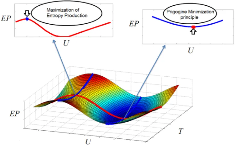
2. Maximization or Minimization of Entropy production?
96
At first sight, Principle B appears in conflict with an established result of Prigogine, according to 97
which the stationary states of a system close to equilibrium are states with minimum entropy 98
production. In fact, both principles can be reconciled if Principle B is viewed as a MaxMin, principle: 99
Martyushev et al. [26] and Kleidon [21] suggest that Prigogine’s principle select the steady state 100
of minimum entropy production compared to transient states. For a steady-state condition, the 101
minimum entropy production principle does not give any further information if many steady state 102
conditions are possible given the imposed boundary conditions. To provide a simple example, let us 103
consider a system characterized by two parameters, T and U, where T controls the departure from 104
equilibrium and U labels an additional constraint of the system, allowing the existence of several 105
stationary states at a given T (see Figure4). In our von Karman system, T could for example label 106
the velocity fluctuations, and U the angular momentum transport. In the T direction, application 107
of the Prigogine principle selects the value of T corresponding to the stationary state. When there 108
are several possible stationary state, the Principle B then selects the most stable state as the one with 109
the largest entropy production, thereby fixing the corresponding value of U. This was precisely the 110
procedure followed by Paltridge. 111
On the other hand, it appears that the stability of the stationary state may depend on boundary 112
conditions. For example, Niven [27] or Kawazura and Yoshida [28] provide explicit examples of 113
out-of-equilibrium systems, in which the entropy production is sl maximized for fixed temperature 114
boundary conditions, while it is minimized for fixed heat flux boundary conditions. In the 115
experimental von Karman system discussed in Section1, we observe a similar phenomenon: for fixed 116
propeller velocities, the selected stationary state is the one of maximum dissipation. However, when 117
one changes the boundary conditions into fixed applied torque at each propeller, the stationary state 118
regime disappears and is replaced by a dynamical regime, in which the system switches between 119
different meta-stable states of low and high energy dissipation [6]. This case is discussed in more 120
detail in Section6. It shows however that we cannot trust the Maximum Entropy Production principle 121
blindly, and must find ways to understand why and when it works, using tools borrowed from 122
Figure 4.Illustration of the relation between maximization of entropy production EP and Prigogine principle: the system is set out of equilibrium by the parameters T and U. T controls the departure from equilibrium and U labels an additional constraint of the system. In the T direction, application of the Prigogine principle selects the value of T corresponding to the stationary state, where MEP selects the one with largest EP in the U direction.
1 2 · · · L Reservoir 1 − p p Reservoir δ β α γ
Figure 5. The dynamical rules of the toy model of scalar transport: the particle can jump to the left or to the right with probabilities denied by p. At both end, two reservoirs sets the flux of incoming or outgoing particles. The particle can be a boson (several particles per box are allowed), in which case the process is called zero-range process (ZRP). When the particle is a fermion, jump towards a box that is already occupied are forbidden. The corresponding process is called asymmetric exclusion process (ASEP).
non-equilibrium theories. A justification has been attempted [8], and dismissed [22,23], following the 123
ideas of Jaynes that non-equilibrium systems should be characterized by a probability distribution 124
on the trajectories in phase space, instead of just the points in phase space at equilibrium. A more 125
pragmatic way to evaluate the validity of Principle B is to consider its application to toy models of 126
non-equilibrium statistics, that mimics the main processes at work in the von Karman flow, and that 127
can guide us on a way to a justification (or dismissal). This is the topic of the next section. 128
3. From Maximum entropy production to Maximum Kolmogorov-Sinai entropy in toy models of
129
turbulence
130
3.1. From passive scalar equation to Markovian box models 131
In the von Karman flow, angular momentum is transported from the vessel ends towards the center. In Rayleigh-Benard, the temperature is transported from the bottom to the top plates. In shear flows, the linear momentum is transported from one side to the other. On Earth, the heat is transported from the equator towards the pole. All this system in which Principle B seems to provide a non-trivial answer have then in common that they deal with the transport of a scalar quantity T by a given velocity field u(x, t), and that may be sketched as:
with appropriate boundary conditions. Here κ is the diffusivity. To transform this process into a 132
tractable toy model, we stick to a one dimensional case and divide the accessible space ` into L 133
boxes. We impose the boundary conditions through two reservoirs located at each end of the chain 134
(mimicking e.g. the top and bottom propeller or solar heat flux at pole and equator). The boxes 135
contains bosonic or fermionic particles that can jump in between two adjacent boxes via decorrelated 136
jumps (to the right or to the left) following a 1D Markov dynamics governed by a coupling with 137
the two reservoirs imposing a difference of chemical potential at the ends. The different jumps are 138
described as follow. At each time step a particle can jump right with probability pwnor jump left with
139
probability(1−p)wn. wn is a parameter depending on the number of particles inside the box and
140
on the nature of particles. Choices of different wn give radically different behaviors. For fermionic
141
particles, it prevents a jump on to a site, if this site is already occupied by a particle. The corresponding 142
process is called Asymmetric Exclusion Process (ASEP). For boson, wn = 1 and the process is called
143
Zero Range Process (ZRP). At the edges of the lattice the probability rules are different: at the left 144
edge a particle can enter with probability α and exit with probability γwnwhereas at the right edge a
145
particle can exit with probability βwnand enter with probability δ.
146
Without loss of generality, we may consider only p ≥ 1/2 which corresponds to a particle flow 147
from the left to the right and note U = 2p−1. After a sufficiently long time the system reaches a 148
non-equilibrium steady state, with a well defined density profile (or fugacity profile) across the boxes 149
ranging between ρa, the density of the left reservoir and ρb, the density of the right reservoir, given by
150
ρa =α(γ+eα)and ρb =δ(β+eδ), where e=1 for ASEP (fermion) and e = −1 for ZRP (boson). In
151
the sequel, we fix γ+α=1 and β+δ=1, and denote∆T=ρa−ρbthe parameter that measures the
152
balance between the input rate of the left reservoir (the equivalent of the heat or momentum injection), 153
and the removal rate of the right reservoir (the equivalent of the heat or momentum dissipation). Once 154
β(say),∆T are fixed, we can compute all the other parameter α, γ and δ of the model. In the sequel,
155
we fix β=0.75, and vary∆T and/or U. 156
Taking the continuous limit of this process, it may be checked that the fugacity Z = ρ/(1+ρ)
of stationary solutions of a system consisting of boxes of size 1L follow the continuous equation [29]: U∂Z ∂x − 1 2L ∂2Z ∂x2 =0, (2)
corresponding to stationary solution of a passive scalar equation with velocity U and diffusivity 2L1. Therefore, the fugacity Z is a passive scalar obeying a convective-diffusion equation. We thus see that U =0 corresponds to a purely conductive regime whereas the larger U the more convective the regime. This toy model therefore mimics in the continuous limit the behavior of scalar transport in the von Karman, Rayleigh-Bénard, Couette or Earth system we are trying to understand. The toy model is a discrete Markov process with 2Lstates. It is characterized by its transition matrix P= (pij)which
is irreducible. Thus, the probability measure on the states converges to the stationary probability measure µ= (µ1stat, ..., µ2L
stat)which satisfies:
µistat = 2L
∑
j=1 µjstat.pji∀i∈ [[1, 2 L]]. (3)This Markov property makes our model simple enough so that exact computations are analytically 157
tractable and numerical simulations are possible up to L = 10 (ASEP model) to L = 1000 (ZRP 158
model) on a laptop computer. The idea now is to apply the Principle B in these toy models, and see 159
what useful information we can derive from it. 160
3.2. Maximum Entropy production in Zero Range and ASymmetric Exclusion Process 162
We turn to the definition of entropy production in our toy model system. For a macroscopic system 163
subject to thermodynamic forces Xiand fluxes Ji, the thermodynamic entropy production is given by:
164 [30,31]: 165 σthermo=
∑
i JiXi (4)The fluxes to consider for a diffusive particles model are fluxes of particles and the thermodynamic 166
forces can be written X = ∆(−ν
T) where T is the temperature and ν the chemical potential
167
proportional to log(ρ)for an ideal gas [30]. So, as the temperature is here fixed, the thermodynamic
168
Entropy production of a given stationary state takes the form: 169
σthermo∝ L
∑
i=1Ji.(log(ρi) −log(ρi+1)) =J.(log(ρ1) −log(ρL)) (5)
where ρ is the stationary density distribution and J = Ji the particle fluxes in the stationary state,
where all fluxes become equal and independent on the site. ρ and J are both (nonlinear) function of U. It is easy to show [32] that this definition is just the continuous limit of the classical thermodynamic entropy production in an ideal gas, that reads:
σthermo= −
Z B−
A+
J(x, t)∂log(ρ(x, t))
∂x dx (6)
In the case of bosonic particles (ZRP model), this entropy production takes an compact analytical shape in the (thermodynamic) limit L→0 [33]:
σ(U) = αU U+γ(log( α U+γ−α) −log( (α+δ)U+γδ U(β−α−δ) +βγ−γδ)) (7)
Because U = 2p−1 ≥ 0 the entropy production is positive if and only if ρa ≤ ρb. This means that
170
fluxes are in the opposite direction of the gradient. We remark than if U =0 then σ(U) =0. Indeed 171
J is proportional to U in this model. Moreover, σ(U)is zero also when ρ1=ρL. This happens when
172
U increases, ρa(U)decreases and ρb(U)increases till they take the same value. Thus it exists U, large
173
enough, for which σ(U) =0. Between these two values of U the entropy production has at least one 174
maximum. By computing numerically the entropy production, we observe in fact that it is also true 175
for the fermionic particles, even though we cannot prove it analytically. This is illustrated in Figure6
176
for L=100 (ZRP) and L=10 (ASEP). 177
The value of UmaxEP(T)at which this maximum occurs depends on the distance to equilibrium of the
system, characterized by the parameter∆T=α−δ. In the case of the ZRP model, it can be computed
as [33]: UmaxEP,ZRP = ∆T 4Mα+3 ∆T2( α+1) 8M2α2(α−1)+o((∆T) 2), (8)
where M = (1+2ρa)(1+2ρb). This means that at equilibrium (∆T = 0, ρa = ρb), the maximum
178
is attained for U = 0, i.e. the symmetric case. Numerical simulations of the ASEP system suggest 179
that this behavior is qualitatively valid also for fermionic particles: the entropy production displays 180
a maximum, that varies linearly in∆T . Such behavior therefore appears quite generic of this class of 181
toy model. When the system is close to equilibrium (∆T 1), the maximum is very near zero, and, 182
the density profile is linear, corresponding to a conductive case. When the system is out-of-equilibrium 183
(∆T≥0) the maximum is shifted towards larger values of U>0, corresponding to a convective state, 184
with flattened profile. An example is provided in Figure7for the ZRP and ASEP model. 185
0 0.1 0.2 0.3 0.4 0.5 0.6 0.7 U 0.6 0.7 0.8 0.9 1 1.1 1.2 Entropy production a) 0 0.1 0.2 0.3 0.4 U 0.6 0.7 0.8 0.9 1 1.1 1.2 1.3 1.4 1.5 1.6 Entropy productions b)
Figure 6.Entropy productions as a function of U for β=0.75 and∆T=0.25 for two toys models. Red stars: Thermodynamic entropy production σ(U); blue squares: Kolmogorov-Sinai entropy hKS(U).
The location of the maxima are denoted by vertical dashed line (red for σ(U); and blue for hKS(U)).
a) Case L=10 ASEP (fermion) ; b) Case L=100 ZRP (boson) . The dot-dashed line is the asymptotic law for σ(U)given by Eq. (7).
0 0.2 0.4 0.6 0.8 1 l/L 0.15 0.2 0.25 0.3 0.35 0.4 0.45 (U maxEP ) a) 0 0.2 0.4 0.6 0.8 1 l/L 0.5 0.55 0.6 0.65 0.7 0.75 (U maxEP ) b)
Figure 7.Profiles of density profiles (blue line) corresponding to models with U=UmaxEPfor β=0.75
and∆T=0.25 for two toys models. The red dashed line is the density profile obtained at U=0, i.e. in the conductive case. a) Case L=10 ASEP (fermion) ; b) Case L=100 ZRP (boson)
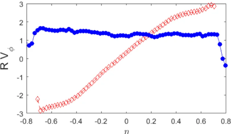
Figure 8.Profiles of angular momentum RVφas a function of the height from the central plane η in the
von Karman laboratory experiment. Blue symbols with line: in the bifurcated state with higher energy dissipation. Red line with symbols: in the symmetric state.
Our toy models are examples of systems with deviation from equilibrium (labelled by∆T), admitting 186
several stationary states (labelled by U). So if we were to apply our MinMax/Principle B to these 187
toy models, we would select the model corresponding to UmaxEP as the most stable one, i.e. the
188
conductive state with linear profile at equilibrium, and the convective state with flattened profile at 189
non-equilibrium. Interestingly enough, this selection corresponds qualitatively to the type of profiles 190
that are selected by the non-linear dynamics in the von Karman, Rayleigh-Benard or Couette system, 191
as illustrated in Figure8for the VK flow: for low levels of fluctuations (low Reynolds or impeller 192
with moderately bent blades) corresponding to close to equilibrium state, the most stable state is the 193
symmetric state, with linear angular momentum profile. At larger fluctuation rates, the most stable 194
state is the bifurcated state, with flat angular momentum at the center. 195
The ability of Principle B, based only on entropy i.e. equilibrium notions, to predict at least 196
qualitatively the correct behavior of scalar transport in several non-equilibrium turbulent system 197
is puzzling. It would be more satisfying to connect this Principle to other notions that seem more 198
appropriate in the case of non-equilibrium system. This is the topic of the next section. 199
3.3. From Maximum Entropy Production to Kolmogorov-Sinai Entropy 200
The physical meaning of the thermodynamic entropy production is the measure of irreversibility: the larger σ the more irreversible the system [34] . It is however only a static quantity, being unconnected to the behavior of trajectories in the phase space. In that respect, it is not in agreement with the ideas of Jaynes that non-equilibrium systems should be characterized by a probability distribution on the trajectories in phase space, instead of just the points in phase space at equilibrium. In the context of Markov chains, Jaynes’ idea provides a natural generalization of equilibrium statistical mechanics [35], by considering the Kolmogorov-Sinai entropy (KSE). There are many ways to estimate the Kolmogorov-Sinai entropy associated with a Markov chain [35,36].The most useful one in our context is the one defined as the time derivative of the Jaynes entropy. To characterize the dynamics of the system during the time interval[0, t], one considers the possible dynamical trajectoriesΓ[0,t] and the
associated probabilities pΓ[0,t]. The dynamical trajectories entropy- the Jaynes entropy- reads: SJaynes(t) = −
∑
Γ[0,t]
0 0.1 0.2 0.3 0.4 0.5 0.6 T 0 0.1 0.2 0.3 0.4 0.5 0.6 U max a) 0 0.05 0.1 0.15 0.2 0.25 0.3 T 0 0.005 0.01 0.015 0.02 0.025 0.03 0.035 0.04 0.045 0.05 U max b)
Figure 9. Location of the maximum of thermodynamic entropy production UmaxEP(red stars) and
maxim of Kolmogorov-Sinai entropy (blue stars) as a function of∆T. a) Case L=10 ASEP (fermion). b) Case L=100 ZRP (boson). The red dashed line is the second order approximation given by Eq. (8). The blue-dashed line is the first order approximation to the location of the maxima ( Eq. (12)).
For a Markov chain we find that:
SJaynes(t) −SJaynes(t−1) = −
∑
(i,j)µistatpijlog(pij) (10)
Thus, the Kolmogorov-Sinai Entropy for the Markov chain is: hKS = −
∑
(i,j)
µistatpijlog(pij), (11)
where µiis the stationary measure and pijthe transition matrix.
201
In the case of bosonic particles (ZRP model), the KSE can be computed analytically and it admits a maximum as a function of U [33]. The value of U corresponding to this maximum can also be computed analytically, and leads to:
UmaxKS =
∆T
4Mα+o(∆T), (12)
Such first order approximation appear to be valid even far from equilibrium (see Figure 9). 202
Comparing with the value for the maximum of entropy production, we see that the two maxima 203
coincide, to first order in∆T and 1/L: in the continuous limit, Principle B provides the same kind of 204
information than a third principle that we may state as: 205
Principle C: In certain non-equilibrium systems with coexistence of several stationary state, the most 206
stable one is that of Maximum Kolmogorov-Sinai Entropy. 207
Is this third principle any better that the principle B? In our toy models, it seems to give the same 208
information than the Principle B: for ZRP, we have shown analytically that the maxima of each 209
principle coincide to first order in∆T and 1/L. Numerical simulation of the ASEP system suggests 210
that it is also true for fermionic particles: for a given value of∆T the difference between the two 211
maxima ∆Umax = UmaxEP −UmaxKS decreases with increasing L [32]. For a fixed L, the difference
between the two maxima increases with∆T, but never exceeds a few percent at L = 10 [32], see 213
Figure9). 214
In turbulent system, the test of this principle is more elaborate, because the computation of hKSis not
215
straightforward. It would however be interesting to test it in numerical simulations. 216
4. From Maximum Kolmogorov-Sinai entropy to Minimum Mixing Time in Markov
217
Chains
218
Principle C is appealing because it involves a quantity clearly connected with dynamics in the phase 219
space, but it is still unclear why the maximization of the entropy associated with paths in the phase 220
space should select the most stable stationary state, if any. To make such a link, we need to somehow 221
connect to the relaxation towards a stationary state, i.e. the time a system takes to reach its stationary 222
state. In Markov chains, such a time is well defined, and is called the mixing time. Intuitively, one 223
may think that the smaller the mixing time, the most probable it is to observe a given stationary state. 224
So there should be a link between the maximum of Kolmogorov-Sinai entropy, and the Minimum 225
mixing time. This link has been derived in [25], for general Markov chains defined by their adjacency 226
matrix A and transition matrix P, defined as follows: A(i, j) =1 if and only if there is a link between 227
the nodes i and j and 0 otherwise. P= (pij)where pijis the probability for a particle in i to hop on
228
the j node. Specifically, it has been shown that Kolmogorov-Sinai entropy increases with decreasing 229
mixing time (see Figure 1 in [25]). More generally, for a given degree of sparseness of the matrix 230
A (number of 0), the Markov process maximizing the Kolmogorov-Sinai entropy is close (using an 231
appropriate distance) to the Markov process minimizing the mixing time. The degree of closeness 232
depends on the sparseness, and becomes very large with decreasing sparseness, i.e. for unconstrained 233
dynamics (Figure 3 in [25]). 234
This result provides us with a fourth principle in Markov chains: 235
Principle D: In certain non-equilibrium systems with coexistence of several stationary states, the 236
most stable one is that of Minimum Mixing Time. 237
238
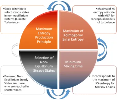
Given what we have seen before, there are 4 general principle that select the same stationary state, 239
in the limit of large size and small deviations from out-of-equilibrium (see Figure10). Among all 4, 240
the Principle that provides the better understanding of its application is the Principle D, because the 241
smaller the mixing time, the less time it is required to reach a given state and so the most probable the 242
corresponding state. This phenomenological understanding can actually be given a deeper meaning 243
when switching from Markov chains to Langevin systems. 244
5. From Minimum Mixing Time in Markov Chains to Mean Escape rate in Langevin
245
systems
246
The notions we have derived in Markov chains have actually a natural counter-part in general Langevin systems. Consider indeed the general Langevin model:
˙x= f(x) +ξ, (13)
where f(x)is the force and ξ is a delta-correlated Gaussian noise:
Figure 10.Conceptual path to demonstrate the validity of the Maximum Entropy Principle followed in this paper.
The probability distribution of x, P(x, t)then obeys a Fokker-Planck equation: 247
∂tP(x, t) = −∂x(f(x)P(x, t)) +D∂x∂xP(x, t),
= ∂x(J(x, t)P(x, t)), (15)
where J= f(x)P(x, t) −D∂xP(x, t)is the current. It is well known (see e.g. [37]) that the discretization
of the Langevin model on a lattice of grid spacing a (so that x= na) is a Markov chain, governed by the master equation:
∂tPn=w+n−1Pn−1−wn+Pn+w−n+1−w−nPn, (16)
where Pnis the probability of having the particle at node n and w±n are the probability of forward and
248
backward jump at node n, given by: 249 w+n = D a2, w−n = D a2− fn a. (17)
From this, we can compute the Kolomogorov-Sinai entropy as [38] hKSL=<w+n ln w+n w−n+1+w − n ln w−n w+n−1 >, (18)
which in the continuous limit a→0 becomes:
hKSLc =<
1 D|f(x)|
2+ f0(x)>, (19)
which is the well know entropy production. 250
On the other hand, the dissipated power in the Langevin process can easily be computed as :
P =< f˙x>=
Z
J(x, t)f(x, t)dx=< |f|2+D f0(x)>=Dh
The Kolmogorov-Sinai entropy and the dissipated power are thus proportional to each other. In such 251
example, it is thus clear that maxima of hKSand maxima of entropy production coincide.
252
On the other hand, when f derives from a potential, f = −∂x(U), there may be several meta-stable
253
positions at U local minima. In such a case, it is known from diffusion maps theory and spectral 254
clustering [39] that the exit times from the meta-stable states are connected to the smallest eigenvalues 255
of the operatorH, such thatHP= D∆P− ∇P∇U, which is the equivalent of the Liouville operator 256
in Markov chain. More specifically, if U has N local minima, then the spectra of H has a cluster 257
of N eigenvalues µ1 < µ2 < .. < µN located near 0, each of which being associated with the exit
258
time it takes to get out from the local minima Sito the state corresponding to the deepest minimum
259
(the equilibrium state). For example, µ1 = τ11, where τ1 is the mean exit time to jump the highest
260
barrier of energy onto the deepest well. We see from that that the smaller the eigenvalue (equivalent 261
to the mixing time), the longer time it takes to jump from this metastable state, and so the more 262
stable is this state. This provides a quantitative justification of the notion that the most stable stationary 263
states are the one with the minimum mixing time. It is worth mentioning that Langevin systems 264
are now incorporated in numerical weather prediction to provide some flexibility to the sub-grid 265
scales parameterizations [40]. Models based on these so-called stochastic parameterizations have 266
usually better prediction skills than models based on deterministic parameterizations. Stochastic 267
parameterization is therefore increasingly used in different aspects of weather and climate modeling 268
[41]. We might speculate that, in these large simulations, the stochasticity helps models to reach more 269
realistic results by favoring jumps to more stable states as outlined above. Another way to select these 270
more realistic states could possibly be to search for the ones that maximize dissipation or entropy 271
production, as was done empirically in a simple way in Paltridge’s model [13,14]. 272
6. Summary: Turbulence as a minimum Mixing Time State?
273
Considering a mixing time to characterize turbulence is natural, given the well known enhancement 274
of mixing properties observed in turbulent flows. The mixing time defined for Markov chains is 275
also comparable to the mixing time one would naturally define for turbulence, namely the smallest 276
time after which a given partition of a scale quantity is uniformly spread over the volume. This time 277
corresponds to the one defined by Arnold for dynamical systems [42] when introducing the concept 278
of strong mixing. Here, it is the time associated with eigenvalues of the Liouville operator of the 279
processes describing the turbulence action. In the specific example we consider here, namely von 280
Karman flow, the turbulence is characterized by a symmetry along the rotation axis, which favors 281
stationary states in which angular momentum is mixed along meridional planes [43,44].In this case, 282
there is a clear connection between the equation obeying the angular momentum and the classical 283
Fokker-Planck equation Eq. (15). One can thus hope in such a case to find a Langevin process 284
describing the angular momentum mixing. This was actually done in [43] and shown to reproduce 285
very well the power statistics in both regimes of constant torque and constant speed forcing, in case 286
where there is only one stationary state. For multiple stationary states, obtained in the regime with 287
fixed applied torque, the corresponding Langevin process has been derived in [45] and it turns out 288
to be a non-linear stochastic oscillator, featuring multiple metastable states and limit cycles. Such 289
oscillator is found to describe the dynamics of the reduced frequency θ = (f1−f2)/(f1+ f2)which
290
is a global observable respecting the symmetries of the flow. The challenge is then to compute the 291
mixing times of the different metastable states arising in the non-linear stochastic oscillator. 292
In [46–48] we have shown that the mixing time τ of turbulent flows can be easily obtained by fitting 293
the Langevin process (or aut-regressive process) xt = φxt−1+ξ(t) to data. Here x(t) is a global
294
quantity tracing the symmetry of the flows, ξ(t)is a random variable normally distributed and−1<
295
φ < 1 is the so called auto-regressive coefficient. The link with the mixing time is made through
296
the parameter|φ|which is indeed proportional to τ: the larger this quantity, the slower the mixing
in the system, because the dynamics weight more the present observation xt when updating xt+1.
298
In [46], only flow configurations with a single stationary state have been analysed and φ computed 299
using the complete time series. To extend the results to the flow regimes featuring multistability, we 300
use the strategy outlined in [49]. First of all, we reconstruct the dynamics by using the embedding 301
methodology on the series of partial maxima of θ, denoted as θi. A 2D section of the attractor is
302
shown in the upper panel of Figure11and it is obtained by plotting θias a function of the subsequent
303
maxima θi+1. The histogram of θiis reported in the lower panel and show the correspondence to three
304
metastable states s1, s2, s3. Since we are not dealing with a stationary process, we cannot compute a
305
single φ for the full time series of θ. The method introduced in [49] consists in computing a value of 306
φifor each θi, taking the 50 previous observations of the complete time series. The distribution of|φ|
307
is shown in colorscale in Figure11. It is evident that the most represented states (s1and s2) are those
308
with the minimum mixing time whereas the most unstable one (s3) is the one with the largest mixing
309
time. This example shows that the results outlined in Section 5 can be extended to higher dimensions 310
and that there is a simple strategy to compute the mixing times in complex systems. 311
It is quite plausible that such study can be generalized to turbulent systems with other symmetry, 312
such as symmetry by translation along an axis. The turbulent shear flow enter in that category. 313
Finally, we note that in Rayleigh-Bénard systems or in stratified turbulence, the temperature is also a 314
quantity that is mixed within the flow, and that should also be liable to a Langevin description. It is 315
therefore not a coincidence that shear flow, Rayleigh-Bénard convection and von Karman flows are 316
so far the only systems in which the principle of Maximum Energy dissipation has been applied with 317
some success. They are systems where a Langevin description is possible, and where the Maximum 318
Energy dissipation principle in fact coincides with the Minimum Mixing time principle, connected 319
to the longest exit time from meta-stable states. As observed by [50], these flows tends to be in 320
a steady state with a distribution of eddies that produce the maximum rate of entropy increase in 321
the nonequilibrium surroundings. In more general turbulence, it is not clear that such a Langevin 322
description is possible, so that the statement of Turbulence as a minimum Mixing Time State might 323
actually be limited to quite special situations, where symmetry or dynamics impose pure mixing 324
of a quantity (like angular momentum, momentum or temperature). Shear flow, Rayleigh Benard 325
convection and von Karman flows belong to this category. 326
Other conceptual pathways allow to link MEP to the underlying dynamics of the system: Moroz 327
[51] suggests that the dissipation time minimization is linked to the least action principle, used 328
in chemistry, biology and physics to derive the equations of motion. Although this theoretical 329
formulation goes in the same direction of the results provided in this paper, our approach provides a 330
rather practical way to connect dynamics and thermodynamics through statistical quantities directly 331
computable from experimental time series. 332
Acknowledgments: M.M. and B.D. were supported by the ANR ECOUTURB. M.M. was supported by a
333
fellowship from the LABEX PALM. DF was supported by ERC grant No. 338965
334
Author Contributions:M.M., B.D. and D.P. conceived and designed the models; B.D., D.F., and M.M. performed
335
the numerical computations; M.M. B.D. and D.F. analyzed the data; all the authors wrote the paper.
336
Conflicts of Interest:The authors declare no conflict of interest.
337
Bibliography
338
1. Malkus, W.V. The heat transport and spectrum of thermal turbulence. Proceedings of the Royal Society
339
of London A: Mathematical, Physical and Engineering Sciences. The Royal Society, 1954, Vol. 225, pp.
340
196–212.
341
2. Malkus, W. Outline of a theory of turbulent shear flow. Journal of Fluid Mechanics 1956, 1, 521–539.
-0.15 -0.1 -0.05 0 0.05 0.1 0.15 0.2 0.25 0.3 0.35
θ
i+1 -0.1 0 0.1 0.2 0.3|
φ
|
0 0.1 0.2 0.3 0.4 0.5 0.6 0.7 0.8 0.9 1θ
i -0.15 -0.1 -0.05 0 0.05 0.1 0.15 0.2 0.25 0.3 0.35f(
θ
)
0 50 100 150 200 250 300 350 400s
1s
2s
3Figure 11. Upper panel: 2D Poincaré section of the Von Karman attractor obtained embedding the partial maxima of the reduced frequency θi. The colors represent|φ|, the autoregressive coefficient computed for each of the θi, using the 50 previous observations of the full time series of θ. Lower
panel: histogram of the partial maxima θi. The metastable state s3is visited less than s1and s2and
3. Spiegel, E.A. Thermal turbulence at very small Prandtl number. Journal of Geophysical Research 1962,
343
67, 3063–3070.
344
4. Marie, L.; Daviaud, F. Experimental measurement of the scale-by-scale momentum transport budget in a
345
turbulent shear flow. Physics of Fluids (1994-present) 2004, 16, 457–461.
346
5. Ravelet, F.; Marié, L.; Chiffaudel, A.; Daviaud, F. Multistability and memory effect in a highly turbulent
347
flow: experimental evidence for a global bifurcation. Physical review letters 2004, 93, 164501.
348
6. Saint-Michel, B.; Dubrulle, B.; Marié, L.; Ravelet, F.; Daviaud, F. Evidence for forcing-dependent steady
349
states in a turbulent swirling flow. Physical review letters 2013, 111, 234502.
350
7. Lorenz, E.N. Generation of available potential energy and the intensity of the general circulation 1960.
351
8. Dewar, R.C. Information theory explanation of the fluctuation theorem, maximum entropy production
352
and self-organized criticality in non-equilibrium stationary states. J. Phys. A: Math. Gen. 2003, 36, 631.
353
9. Moroz, A. On a variational formulation of the maximum energy dissipation principle for non-equilibrium
354
chemical thermodynamics. Chemical Physics Letters 2008, 457, 448–452.
355
10. Moroz, A. A variational framework for nonlinear chemical thermodynamics employing the maximum
356
energy dissipation principle. The Journal of Physical Chemistry B 2009, 113, 8086–8090.
357
11. Ziegler, H. Progress in Solid Mechanics, ed. IN Sneddon and R. Hill. Amsterdam, The Netherlands:
358
North-Holland Publishing Co 1963, 4, 93.
359
12. Ziegler, H.; Wehrli, C. The derivation of constitutive relations from the free energy and the dissipation
360
function. Advances in applied mechanics 1987, 25, 183–238.
361
13. Paltridge, G.W. Global dynamics and climate-a system of minimum entropy exchange. Q. J. R. Meteorol.
362
Soc. 1975, 101, 475–484.
363
14. Herbert, C.; Paillard, D.; Kageyama, M.; Dubrulle, B. Present and Last Glacial Maximum climates as
364
states of maximum entropy production. Q. J. R. Meteorol. Soc. 2011, 137, 1059–1069.
365
15. Kleidon, A.; Fraedrich, K.; Kunz, T.; Lunkeit, F. The atmospheric circulation and states of maximum
366
entropy production. Geophysical research letters 2003, 30.
367
16. Lorenz, R.D.; Lunine, J.I.; Withers, P.G.; McKay, C.P. Titan, Mars and Earth: Entropy production by
368
latitudinal heat transport. Geophysical Research Letters 2001, 28, 415–418.
369
17. Lorenz, R.D. Maximum frictional dissipation and the information entropy of windspeeds. Journal of
370
Non-Equilibrium Thermodynamics 2002, 27, 229–238.
371
18. Ozawa, H.; Ohmura, A. Thermodynamics of a global-mean state of the atmosphere—a state of maximum
372
entropy increase. Journal of climate 1997, 10, 441–445.
373
19. Shimokawa, S.; Ozawa, H. On the thermodynamics of the oceanic general circulation: Irreversible
374
transition to a state with higher rate of entropy production. Quarterly Journal of the Royal Meteorological
375
Society 2002, 128, 2115–2128.
376
20. Ozawa, H.; Ohmura, A.; Lorenz, R.D.; Pujol, T. The second law of thermodynamics and the global climate
377
system: a review of the maximum entropy production principle. Reviews of Geophysics 2003, 41.
378
21. Kleidon, A. Nonequilibrium thermodynamics and maximum entropy production in the Earth system.
379
Naturwissenschaften 2009, 96, 1–25.
380
22. Grinstein, G.; Linsker, R. Comments on a derivation and application of the ‘maximum entropy
381
production’ principle. J. Phys. A 2007, 40, 9717–9720.
382
23. Bruers, S. A discussion on maximum entropy production and information theory. J. Phys. A 2007,
383
40, 7441–7450.
384
24. Gaspard, P.; Nicolis, G. Transport properties, Lyapunov exponents, and entropy per unit time. Physical
385
review letters 1990, 65, 1693.
386
25. Mihelich, M.; Dubrulle, B.; Paillard, D.; Faranda, D.; Kral, Q. Maximum Kolmogorov-Sinai entropy vs
387
minimum mixing time in Markov chains. arXiv preprint arXiv:1506.08667 2015.
388
26. Martyushev, L.M.; Seleznev, V.D. Maximum entropy production principle in physics, chemistry and
389
biology. Phys. Rep. 2006, 426, 1–45.
390
27. Niven, R.K. Simultaneous extrema in the entropy production for steady-state fluid flow in parallel pipes.
391
Journal of Non-Equilibrium Thermodynamics 2010, 35, 347–378.
392
28. Kawazura, Y.; Yoshida, Z. Comparison of entropy production rates in two different types of self-organized
393
flows: Bénard convection and zonal flow. Physics of Plasmas 2012, 19, 012305.
29. Levine, E.; Mukamel, D.; Schütz, G. Zero-range process with open boundaries. Journal of statistical physics
395
2005, 120, 759–778.
396
30. Balian, R. Physique statistique et themodynamique hors équilibre; Ecole Polytechnique, 1992.
397
31. De Groot, S.; Mazur, P. Non-equilibrium thermodynamics; Dover publications, 2011.
398
32. Mihelich, M.; Dubrulle, B.; Paillard, D.; Herbert, C. Maximum Entropy Production vs. Kolmogorov-Sinai
399
Entropy in a Constrained ASEP Model. Entropy 2014, 16, 1037–1046.
400
33. Mihelich, M.; Faranda, D.; Dubrulle, B.; Paillard, D. Statistical optimization for passive scalar transport:
401
maximum entropy production versus maximum Kolmogorov–Sinai entropy. Nonlinear Processes in
402
Geophysics 2015, 22, 187–196.
403
34. Prigogine, I. Thermodynamics of irreversible processes; Thomas, 1955.
404
35. Monthus, C. Non-equilibrium steady states: maximization of the Shannon entropy associated with the
405
distribution of dynamical trajectories in the presence of constraints. J. Stat. Mech. 2011, p. P03008.
406
36. Billingsley, P. Ergodic theory and information; Wiley, 1965.
407
37. Tomé, T.; de Oliveira, M.J. Entropy production in irreversible systems described by a Fokker-Planck
408
equation. Physical Review E 2010, 82, 021120.
409
38. Lebowitz, J.L.; Spohn, H. A Gallavotti–Cohen-type symmetry in the large deviation functional for
410
stochastic dynamics. Journal of Statistical Physics 1999, 95, 333–365.
411
39. Nadler, B.; Lafon, S.; Coifman, R.R.; Kevrekidis, I.G. Diffusion maps, spectral clustering and
412
eigenfunctions of Fokker-Planck operators. arXiv preprint math/0506090 2005.
413
40. Palmer, T.N. A nonlinear dynamical perspective on model error: A proposal for non-local
414
stochastic-dynamic parametrization in weather and climate prediction models. Quarterly Journal of the
415
Royal Meteorological Society 2001, 127, 279–304.
416
41. Berner, J.; Achatz, U.; Batte, L.; Bengtsson, L.; De La Camara, A.; Christensen, H.M.; Colangeli, M.;
417
Coleman, D.R.; Crommelin, D.; Dolaptchiev, S.I.; others. Stochastic parameterization: towards a new
418
view of weather and climate models. Bulletin of the American Meteorological Society 2016.
419
42. Arnold, V.I.; Avez, A. Ergodic problems of classical mechanics; Vol. 9, Benjamin, 1968.
420
43. Leprovost, N.; Marié, L.; Dubrulle, B. A stochastic model of torques in von Karman swirling flow. The
421
European Physical Journal B-Condensed Matter and Complex Systems 2004, 39, 121–129.
422
44. Monchaux, R.; Cortet, P.P.; Chavanis, P.H.; Chiffaudel, A.; Daviaud, F.; Diribarne, P.; Dubrulle, B.
423
Fluctuation-dissipation relations and statistical temperatures in a turbulent von Kármán flow. Physical
424
review letters 2008, 101, 174502.
425
45. Faranda, D.; Sato, Y.; Saint-Michel, B.; Wiertel, C.; Padilla, V.; Dubrulle, B.; Daviaud, F. Stochastic chaos
426
in a turbulent swirling flow. arXiv preprint arXiv:1607.08409 2016.
427
46. Faranda, D.; Pons, F.M.E.; Dubrulle, B.; Daviaud, F.; Saint-Michel, B.; Herbert, É.; Cortet, P.P. Modelling
428
and analysis of turbulent datasets using Auto Regressive Moving Average processes. Physics of Fluids
429
(1994-present) 2014, 26, 105101.
430
47. Faranda, D.; Pons, F.M.E.; Giachino, E.; Vaienti, S.; Dubrulle, B. Early warnings indicators of financial
431
crises via auto regressive moving average models. Communications in Nonlinear Science and Numerical
432
Simulation 2015, 29, 233–239.
433
48. Faranda, D.; Defrance, D. A wavelet-based approach to detect climate change on the coherent and
434
turbulent component of the atmospheric circulation. Earth System Dynamics 2016, 7, 517–523.
435
49. Nevo, G.; Vercauteren, N.; Kaiser, A.; Dubrulle, B.; Faranda, D. A statistical-mechanical approach to study
436
the hydrodynamic stability of stably stratified atmospheric boundary layer 2016.
437
50. Ozawa, H.; Shimokawa, S.; Sakuma, H. Thermodynamics of fluid turbulence: A unified approach to the
438
maximum transport properties. Physical Review E 2001, 64, 026303.
439
51. Moroz, A. The common extremalities in biology and physics: maximum energy dissipation principle in chemistry,
440
biology, physics and evolution; Elsevier, 2011.
441
c
2017 by the authors. Submitted to Entropy for possible open access publication
442
under the terms and conditions of the Creative Commons Attribution (CC BY) license
443
(http://creativecommons.org/licenses/by/4.0/).

![Figure 3. Spontaneous bifurcation in the von Karman flow: the flow, initially started in a symmetrical state, bifurcates after a certain time toward a bifurcated state, that produces a 4 times larger dissipation [5]](https://thumb-eu.123doks.com/thumbv2/123doknet/13095192.385640/5.892.124.766.327.800/spontaneous-bifurcation-initially-symmetrical-bifurcates-bifurcated-produces-dissipation.webp)