HAL Id: hal-01852849
https://hal-amu.archives-ouvertes.fr/hal-01852849
Submitted on 2 Aug 2018HAL is a multi-disciplinary open access
archive for the deposit and dissemination of sci-entific research documents, whether they are pub-lished or not. The documents may come from teaching and research institutions in France or abroad, or from public or private research centers.
L’archive ouverte pluridisciplinaire HAL, est destinée au dépôt et à la diffusion de documents scientifiques de niveau recherche, publiés ou non, émanant des établissements d’enseignement et de recherche français ou étrangers, des laboratoires publics ou privés.
Urban Vegetation Mapping using Hyperspectral
Imagery and Spectral Library
Walid Ouerghemmi, Sébastien Gadal, Gintautas Mozgeris
To cite this version:
Walid Ouerghemmi, Sébastien Gadal, Gintautas Mozgeris. Urban Vegetation Mapping using Hyper-spectral Imagery and Spectral Library. IEEE International Geoscience and Remote Sensing Sympo-sium (IGARSS) 2018, IEEE, Jul 2018, Valencia, Spain. pp.1632-1635. �hal-01852849�
URBAN VEGETATION MAPPING USING HYPERSPECTRAL IMAGERY AND SPECTRAL
LIBRARY
Walid Ouerghemmi
1, Sébastien Gadal
1, Gintautas Mozgeris
21Aix-Marseille Univ, CNRS, ESPACE UMR 7300, Univ Nice Sophia Antipolis, Avignon Univ, 13545 Aix-en-Provence, France 2Aleksandras Stulginskis University, LT-53361, Kaunas r., Lithuania
ABSTRACT
The development and expansion of urbanized areas around the cities, brings new challenging issues about the organization, the monitoring, and the distribution of green spaces within the cities (e.g. grass, trees, shrubs, etc.). Indeed, these spaces brings better life quality for population and preserve biodiversity. This study, aims to 1) investigate the feasibility of urban vegetation mapping by species using multiband imagery and spectral libraries and to 2) determine at what scale the mapping is reliable (e.g. trees scale, group of trees scale, high/short vegetation scale).
Index Terms— Hyperspectral, spectral library, band
selection, regularization, vegetation mapping.
1. INTRODUCTION
Urban vegetation study is a key feature in landscape monitoring; it serves as an ecological regulator, and provides many ecosystem services. The preservation and management of the green spaces requires an accurate mapping, which is carried by field inspection, aerial photography interpretation, and other time and money-consuming methods. The existing solutions of urban vegetation inventories may be significantly improved by introducing more advanced remote sensing techniques without notable increase of costs. Vegetation mapping and monitoring in urban context by remote sensing, remains nevertheless, a challenging issue, insofar as the vegetation spectral response is sensitive to chlorophyll content at the plant level, which increase spectral variability regarding individual species. Many misclassifications between species could be therefore expected depending on the seasonality, data spectral/spatial resolution (e.g. [1], [2]). The goal is to provide reliable vegetation maps that could serve as basis for urban planners, municipalities, and decision makers.
Many existing studies assessed the feasibility of vegetation mapping using remote sensing data (e.g. [3],[4],[5]), however, most of these studies concentrate on specific vegetation families. Few studies addressed the separability issues between species or group of species were, and the spectral correlations issues management.
This study further elaborates on the existing vegetation mapping methods, aiming to propose an original approach, which includes a three steps procedure; 1) a classification step by spectral library, 2) a band selection step for spectral
correlation compensation, and 3) a regularization step, which is applied over the classification map to smooth the rendering.
2. MATERIALS AND METHOD 2.1. Airborne hyperspectral imagery and study zone
For this study, two airborne multiband images were used. The images were acquired using a Vis-NIR sensor (RIKOLA, SENOP OPTRONICS) operating in the spectral range of 500-900nm over the city of Kaunas (Lithuania). For the first campaign in July 2015, the sensor was configured to produce 16 bands for each frame image, a photogrammetrically processed mosaic of size 3189×3292 pixels was used for this study, and the corresponding ground sample distance (GSD) was of 0.7m. For the second campaign in September 2016, the sensor was configured to produce 64 bands for each frame; a mosaic of size 4000×1900 pixels was used for this study. The radiometric calibration was carried using the sensor software, the atmospheric correction was carried using the MODTRAN radiative transfer model [6].
Kaunas city is characterized by a high species diversity with up to 96 tree species, 49 shrubs and 2 vines [7]. For this study, we have focused on the city center zone, the mapping considered urban vegetation of residential gardens, public parks, city trees. The vegetation species were defined using a 2 levels hierarchy, the first level concerns grass (e.g. short vegetation), deciduous trees, and coniferous trees. The second level, which is a finer level, concerns 10 species of deciduous and coniferous trees in addition to grass.
2.2. Urban spectral library
The spectral library includes 50 common urban objects that were collected over the city of Kaunas [8]; the objects include manmade, vegetation and bare soil materials. The measurements were done in laboratory using Themis-Vision VNIR400H sensor. The spectral interval varies from 400 nm to 1000 nm with 1024 narrow bands; the spectral resolution is equal to 0.6 nm. Ten trees species and a short vegetation sample were extracted from the library as follow; 6 deciduous trees including Horse chestnut, European beech, Linden, Maple, Mountain ash, Oak, 4 coniferous trees including Norway spruce, Lime glow, Scots pine, Arborvitae, and 1 green short grass/lawn specie, used in public parks and football field in Kaunas. The ground truth polygons were extracted from a tree inventory of 2012 [9].
The method is articulated around 3 main steps (i.e. Fig.1); the first step concerns the spectral classification and includes; 1) data preprocessing with radiometric and atmospheric corrections, noise reduction using Minimum Noise Fraction method (MNF) [10], and NDVI thresholding which was applied to limit the risk of potential false alarms regarding non-vegetation pixels (e.g. [11]). 2) Classification by Spectral Angle Mapper (SAM) [12], trained with external spectral library or image based spectra. (3) Validation using a trees inventory of individual vegetation species/groups of species. The second step includes a band selection step before applying the SAM classifier to enhance class’s recognition and compensate the high interclass correlation between the vegetation species. The last step consists in applying a regularization method over the classification map generated by the SAM classifier.
For the second step, the BandMax algorithm [13] was used to carry the band selection step. The algorithm is based on the estimation of a separability values for each spectral band; once the background and target spectra defined, the ratios of background and target spectra respectively and , 𝑟𝑏 𝑟𝑡
are calculated as follow for a pair of bands and ;𝑏𝑐 𝑏𝑓
, (1) 𝑟𝑏(𝑛) = 𝑅(𝑏𝑐) 𝑅(𝑏𝑓) 𝑟𝑡(𝑛) = 𝑅(𝑏𝑐) 𝑅(𝑏𝑓)∀ 𝑅
(
𝑏𝑐)
< 𝑅(
𝑏𝑓)
Where 𝑅(𝑏) ∈ [0,1] the reflectance value at band , the 𝑏 𝑛 number of band pairs from which the ratios are calculated, 𝑏𝑐
the current band, and one of the available band 𝑏𝑓 ∀ 𝑏𝑐≠ 𝑏𝑓. Once the ratios calculated for both background and target 𝑛 spectra, the band significance is calculated as the maximum of the difference between both ratios and of all the 𝑟𝑏 𝑟𝑡
defined pair bands:
(2) 𝑆(𝑏𝑐) = 𝑀𝑎𝑥(
‖
𝑟𝑏(𝑛) ‒ 𝑟𝑡(𝑛)‖
)For the third step, a regularization framework was used to smooth the classification rendering, the framework is based on a graphical model, which minimizes an energy function by a graph-cut method named pseudo-Boolean optimization method (QPBO) (e.g. [14]). The energy model is a probabilistic graph function of the membership probability generated after the classification procedure. For 𝑃 this study, we implemented a simplified version of the model used in [15]. For a classification map , the energy term is 𝐶 written as follow: = (3) 𝐸(𝑃, 𝐶) ∑ 𝑥 ∈ 𝐼𝑀𝐸𝑑(𝐶(𝑥)) + 𝜆∑𝑥,𝑦 ∈ 𝑁𝐸𝑟(𝐶(𝑥),𝐶(𝑦)) with (4) 𝐸𝑑(𝐶(𝑥)) = 1 ‒ log (𝑃(𝐶(𝑥))) 𝑃(𝐶(𝑥))𝑡 ∈ [0, 1] =0 (5) 𝐸𝑟𝑒𝑔𝑢𝑙(𝐶(𝑥) = 𝐶(𝑦)) (6) 𝐸𝑟𝑒𝑔𝑢𝑙(𝐶(𝑥) ≠ 𝐶(𝑦)) = 1 ‒ 𝑃(𝐶(𝑥))𝛽
Where 𝐼𝑀 is the multiband input image, 𝜆 ∈ [0,∞[ is an adjustment parameter between data and regularization terms, is the connexity neighbors of x, is an adjustment
𝑁 𝛽 ∈ [0,∞[
parameter between the smoothing level and the importance of in the model. is a function of the membership probability 𝐶 𝐸𝑑
which models the result of the classification map C, if 𝑃
is high, is likely to belong to class and 𝑃(𝐶(𝑥)) 𝑥 𝐶(𝑥) 𝐸𝑑
will be small, conversely, if 𝑃(𝑥) is low, the energy will be near its maximum, and will penalize such configuration. 𝐸𝑟
expresses the relationship between a pixel and its N neighbors. and allows to smooth the initial classification map , by favoring the neighboring pixels to belong to the same 𝐶
class. When 𝐶(𝑥) ≠ 𝐶(𝑦), if 𝑃(𝐶(𝑥)) is high, 𝐸𝑟𝑒𝑔𝑢𝑙 will be near its minimum, and the configuration is likely to be kept, conversely, if 𝑃(𝐶(𝑥)) is low, 𝐸𝑟𝑒𝑔𝑢𝑙 will be high, and the configuration is prone to be rejected.
Fig.1. Vegetation mapping with band selection and regularization steps.
3. VEGEATATION MAPPING RESULTS
3.1. Vegetation species identification by spectral library
The mapping was applied using SAM classifier with a maximum angle in radian equal to 0.1, as a threshold for spectral matching. For each specie, the classifier was trained using 10, 50, and 100 samples. The samples were averaged and resampled to the spectral resolution of the input images.
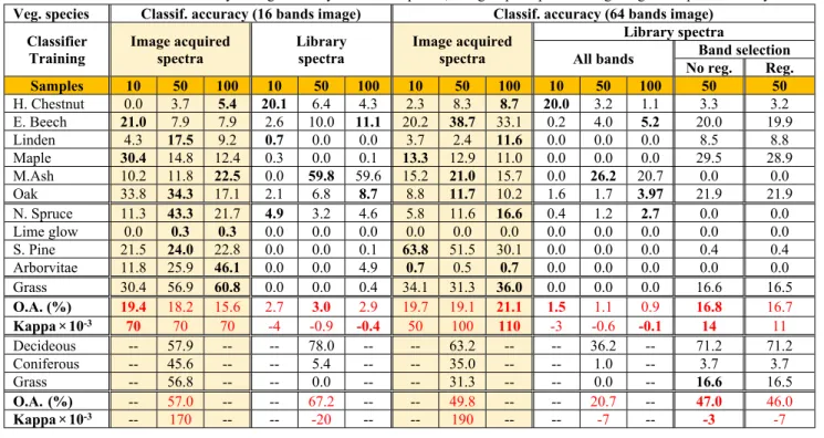
The best overall accuracies for image-based classification were of 19.4% and 21.1%, respectively for 16 and 64 bands images (i.e. Tab.1). Most of the species were recognized with moderate to poor accuracies. The increase of training samples has decreased the classification accuracy for the 16 bands case, conversely, for the 64 bands case, the classification accuracy has increased. This is due to a better spectral characterization of the pixels when increasing the bands number, indeed, the intraclass variability was less impacted when increasing the training samples, and the differentiation between classes was more efficient with less risk of misclassification. The species group classification gives acceptable accuracies for deciduous, coniferous and grass, for both 16 and 64 bands cases.
Concerning the spectral library classification (i.e. Tab.1), the best overall accuracies were of 3.0% and 1.5%, respectively for 16 and 64 bands images. The degree of
species recognition was limited, with at most, a poor detection accuracy. An important decrease was noticeable compared to image based classification, which could be explained –in part- by a lack of spectral concordance between both image and library spectra, indeed, the acquisition conditions were different between both cases. The overall accuracy was poor for the 3 classification training strategies, with a slight enhancement using 50 samples. From these results, the deciduous trees seemed to be better identified than the coniferous ones. In the other hand, some of the coniferous trees were associated to limited pixels of validation, which explain the poor detection of these tree species. The classifier was not able to distinguish grass pixels from tree ones.
The classification by group of vegetation species (i.e. Tab.1) using image based training spectra was acceptable, with global accuracies of 57.0% and 49.8%, respectively for 16 and 64 bands images, deciduous trees were better detected than coniferous and grass. Concerning the spectral library classification, the results were encouraging for the 16 bands case; the deciduous trees were well recognized while coniferous ones were still poorly recognizable. The 64 bands case was less efficient with moderate detection of deciduous
trees, the coniferous trees recognition remains poor.
3.2. Vegetation species identification by bands selection
A band selection was carried over the 64 bands image to enhance classification accuracy and compensate spectral correlation between species. To assess the feasibility of band selection using our spectral library, we applied the BandMax algorithm as follow; the available library trees spectra were defined as target, 5 grass spectra extracted from the image were defined as background. The algorithm detected 15 significant bands that are potentially able to distinguish target spectra from background ones.
The correspondent classification (i.e. Tab.1) permits to increase the deciduous trees detection except for mountain-ash specie. The detection of coniferous were still poor, the grass accuracy increased from 0.0% to 16.6% and the overall accuracy increased from 1.1% to 16.8%.
The classification by group of vegetation species using band selection (i.e. Tab.1), increased significantly the global accuracy from 20.7% to 47.0%, the deciduous trees detection raised from 36% to 71.2%, and coniferous trees accuracy showed a slight increase from 1.0 to 3.7%.
Fig. 2. a) 64 bands image RGB portion with ground truth, b) clean RGB, c) classification by spectral library using all bands, d) classification by spectral library using selected bands, and e) classification by spectral library using selected bands, with regularization step.
3.3. Regularization of the classification map
The classification maps obtained in the previous sections included “salt and pepper” effect (e.g. Fig.2.c-d), due to misclassifications of some pixels. The effect was even more marked over the zones where species are mixed together. The goal here is not necessarily to enhance the classification accuracy, even if it is possible to slightly do so as proved in [15] depending on the context and objects of interest. The regularized map shows a better rendering (Fig.2.e), the classes are better delineated, and many misclassified pixels are eliminated. The global accuracy remains almost the same (i.e. constancy, slight decrease or slight increase).
4. CONCLUSION
This paper proposes an original vegetation mapping method based on the use of an external spectral library for the training process and a classification regularization step. The direct use of the library gives poor species recognition due to unbalanced spectral properties between the spectral library and the multiband image. The spectral balancing was corrected in a second step using a band selection method, the
overall accuracy was enhanced and the performance got closer to the conventional supervised image classification. The deciduous trees were better detected than the coniferous ones. The coniferous trees were poorly detected due to high correlation with deciduous ones. The grass could not be detected using our library, probably because of a poor representativeness of our measured species towards the study zone. In parallel, aggregation of species into 3 vegetation groups resulted in increased accuracy detection of deciduous and coniferous trees. Finally, regularization enhanced the visual rendering of the resulting map.
The vegetation species detection using Vis-NIR imagery is a delicate process involving high spectral correlation between species in addition to their heterogonous distribution over the cities. Nevertheless, the use of a band selection method coupled to a regularization process provided an idea about the spatial localization of the species; high spectral resolution images could be an encouraging tool for vegetation species mapping by spectral library, less spectral resolution is nevertheless sufficient for group of species mapping. To consolidate the validation of the generated maps, a
confrontation with urban planners and vegetation experts must be however considered. In parallel, further
enhancements can be made by testing other band selection methods or other classifiers, and by consolidating the library.
Table I. Classification accuracy of vegetation by individual species, and group of species using image and spectral library.
4. AKNOWLEDGMENTS
This research was supported by the French National Research Agency (ANR) through the HYEP project (ANR-14-CE22- 0016). A special thanks to the National Institute of Geographic and Forestry Information who provided us with the original regularization code.
5. REFERENCES
[1] L. Kumar and P. Sinha, « Mapping salt-marsh land-cover vegetation using high-spatial and hyperspectral satellite data to assist wetland inventory », GIScience & Remote Sensing, vol. 51, no
5, p. 483-497, sept. 2014.
[2] C. Zhang, “Combining hyperspectral and LiDAR data for vegetation mapping in the Florida Everglades,” Photogramm Eng Remote Sens 80:733–743, 2014.
[3] Q. Feng, J. Liu, and J. Gong, “UAV Remote Sensing for Urban Vegetation Mapping Using Random Forest and Texture Analysis,” Remote Sens. 2015, 7, 1074-1094.
[4] E. Belluco, M. Camuffo, S. Ferrari, L. Modenese, S. Silvestri, A. Marani, and M. Marani, “Mapping salt-marsh vegetation by multispectral and hyperspectral remote sensing,” Remote Sensing of Environment 105, 54–67, 2006.
[5] C. Zhang, Z. Xie, “Object-based vegetation mapping in the Kissimmee River watershed using HyMap data and machine learning techniques,” Wetlands 2013, 33, 233–244, 2013. [6] M.W. Matthew, S.M. Adler-Golden, A. Berk, S.C. Richtsmeier, R.Y. Levine, L.S. Bernstein, et al? “Status of atmospheric correction using a MODTRAN4-based algorithm,” SPIE proceeding. Algorithms for multispectral, hyperspectral, and ultraspectral imagery VI, 4049. (pp. 199−207), 2000.
[7] G. Mozgeris, S. Gadal, D. Jonikavičius, L. Straigytė, W. Ouerghemmi and V. Juodkienė, "Hyperspectral and color-infrared imaging from ultralight aircraft: Potential to recognize tree species in urban environments," 2016 8th Workshop on Hyperspectral
Image and Signal Processing: Evolution in Remote Sensing (WHISPERS), Los Angeles, CA, pp. 1-5, 2016.
[8] W. Ouerghemmi, S. Gadal, G. Mozgeris, D. Jonikavičius and C. Weber, "Urban objects classification by spectral library: Feasibility and applications," 2017 Joint Urban Remote Sensing Event
(JURSE), Dubai, pp. 1-4, 2017.
[9] L. Straigytė, T.Vaidelys, “Inventory of green spaces and woody plants in the urban landscape in Ariogala”, South-East European
Forestry, Vol. 3, no. 2, pp. 115-121, 2012.
[10] A.A. Green, M. Berman, P. Switzer, M.D. Craig, “A transformation for ordering multispectral data in terms of image quality with implications for noise removal,” IEEE Trans. Geosci. Remote Sens., 26, 65–74, 1988.
[11] S. Aksoy, H. G. Akcay and T. Wassenaar, "Automatic Mapping of Linear Woody Vegetation Features in Agricultural Landscapes Using Very High Resolution Imagery," in IEEE Transactions on
Geoscience and Remote Sensing, vol. 48, no. 1, pp. 511-522, 2010.
[12] F. A. Kruse, A. B. Lefkoff, J. B. Boardman, K. B. Heidebrecht, A. T. Shapiro, P. J. Barloon, and A. F. H. Goetz, “The Spectral Image Processing System (SIPS) – Interactive Visualization and Analysis of Imaging spectrometer Data.” Remote Sensing of Environment, v. 44, p. 145 – 163, 1993.
[13] Exelis Visual Information Solutions. 2013. High Level Description of the BandMax Algorithm. Boulder, Colorado: Exelis Visual Information Solutions. p.946. [14] Y. Boykov, and V. Kolmogorov, “An experimental comparison of min-cut/max-flow algorithms for energy minimization in vision,”
IEEE Trans. on Pattern Analysis and Machine Intelligence, 26(9),
1124-1137, 2004.
[15] W. Ouerghemmi, A. Le_Bris, N. Chehata, C. Mallet, A two-step decision fusion strategy: application to hyperspectral and multispectral images for urban classification, Int. Arch. Photogramm. Remote Sens. Spatial Inf. Sci., XLII-1/W1, 167-174, 2017.
Veg. species Classif. accuracy (16 bands image) Classif. accuracy (64 bands image)
Library spectra
Band selection Classifier
Training Image acquired spectra Libraryspectra Image acquired spectra All bands No reg. Reg.
Samples 10 50 100 10 50 100 10 50 100 10 50 100 50 50 H. Chestnut 0.0 3.7 5.4 20.1 6.4 4.3 2.3 8.3 8.7 20.0 3.2 1.1 3.3 3.2 E. Beech 21.0 7.9 7.9 2.6 10.0 11.1 20.2 38.7 33.1 0.2 4.0 5.2 20.0 19.9 Linden 4.3 17.5 9.2 0.7 0.0 0.0 3.7 2.4 11.6 0.0 0.0 0.0 8.5 8.8 Maple 30.4 14.8 12.4 0.3 0.0 0.1 13.3 12.9 11.0 0.0 0.0 0.0 29.5 28.9 M.Ash 10.2 11.8 22.5 0.0 59.8 59.6 15.2 21.0 15.7 0.0 26.2 20.7 0.0 0.0 Oak 33.8 34.3 17.1 2.1 6.8 8.7 8.8 11.7 10.2 1.6 1.7 3.97 21.9 21.9 N. Spruce 11.3 43.3 21.7 4.9 3.2 4.6 5.8 11.6 16.6 0.4 1.2 2.7 0.0 0.0 Lime glow 0.0 0.3 0.3 0.0 0.0 0.0 0.0 0.0 0.0 0.0 0.0 0.0 0.0 0.0 S. Pine 21.5 24.0 22.8 0.0 0.0 0.1 63.8 51.5 30.1 0.0 0.0 0.0 0.4 0.4 Arborvitae 11.8 25.9 46.1 0.0 0.0 4.9 0.7 0.5 0.7 0.0 0.0 0.0 0.0 0.0 Grass 30.4 56.9 60.8 0.0 0.0 0.4 34.1 31.3 36.0 0.0 0.0 0.0 16.6 16.5 O.A. (%) 19.4 18.2 15.6 2.7 3.0 2.9 19.7 19.1 21.1 1.5 1.1 0.9 16.8 16.7 Kappa×10-3 70 70 70 -4 -0.9 -0.4 50 100 110 -3 -0.6 -0.1 14 11 Decideous -- 57.9 -- -- 78.0 -- -- 63.2 -- -- 36.2 -- 71.2 71.2 Coniferous -- 45.6 -- -- 5.4 -- -- 35.0 -- -- 1.0 -- 3.7 3.7 Grass -- 56.8 -- -- 0.0 -- -- 31.3 -- -- 0.0 -- 16.6 16.5 O.A. (%) -- 57.0 -- -- 67.2 -- -- 49.8 -- -- 20.7 -- 47.0 46.0 Kappa×10-3 -- 170 -- -- -20 -- -- 190 -- -- -7 -- -3 -7 1635