HAL Id: hal-01777123
https://hal.inria.fr/hal-01777123
Submitted on 24 Apr 2018
HAL is a multi-disciplinary open access
archive for the deposit and dissemination of
sci-entific research documents, whether they are
pub-lished or not. The documents may come from
L’archive ouverte pluridisciplinaire HAL, est
destinée au dépôt et à la diffusion de documents
scientifiques de niveau recherche, publiés ou non,
émanant des établissements d’enseignement et de
MMFilter: A CHR-Based Solver for Generation of
Executions under Weak Memory Models
Allan Blanchard, Nikolai Kosmatov, Frédéric Loulergue
To cite this version:
Allan Blanchard, Nikolai Kosmatov, Frédéric Loulergue. MMFilter: A CHR-Based Solver for
Gen-eration of Executions under Weak Memory Models. Computer Languages, Systems and Structures,
Elsevier, 2018, 53, pp.121-142. �10.1016/j.cl.2018.03.002�. �hal-01777123�
MMFilter: A CHR-Based Solver for Generation of
Executions under Weak Memory Models
Allan Blancharda,∗, Nikolai Kosmatovb,∗, Fr´ed´eric Loulerguec,∗ aInria Lille - Nord Europe, Villeneuve d’Ascq, France
bCEA, List, Software Reliability Laboratory, PC 174, 91191 Gif-sur-Yvette France cNorthern Arizona University, School of Informatics, Computing, and Cyber Systems,
Flagstaff, USA
Abstract
With the wide expansion of multiprocessor architectures, the analysis and rea-soning for programs under weak memory models has become an important con-cern. This work presents MMFilter, an original constraint solver for generating program behaviors respecting a particular memory model. It is implemented in Prolog using CHR (Constraint Handling Rules). The CHR formalism provides a convenient generic solution for specifying memory models. It benefits from the existing optimized implementations of CHR and can be easily extended to new models. We present MMFilter design, illustrate the encoding of memory model constraints in CHR and discuss the benefits and limitations of the proposed technique.
Keywords: weak memory models, constraint solving, logic programming, constraint handling rules
1. Introduction
Concurrent programs are hard to design and implement, especially when running on multiprocessor architectures. For efficiency reasons, multiprocessors implement weak memory models [1] that allow, for example, instruction re-ordering or store buffering. Thus multiprocessors exhibit more behaviors than Lamport’s Sequential Consistency (SC) [18], a theoretical model where an ex-ecution of a parallel program corresponds to an interleaving of exex-ecutions of different threads.
A memory model describes how a program can interact with memory during its execution. Technical manuals of processors are often vague, and sometimes
∗Corresponding author
Email addresses: [email protected] (Allan Blanchard),
[email protected] (Nikolai Kosmatov), [email protected] (Fr´ed´eric Loulergue)
p0: Thread 0 (i00) x = 1; (i01) r0= y; Thread 1 (i10) y = 1; (i11) r1= x; p1: Thread 0 (i000) x = 1; (i001) fence; (i0 02) r0= y; Thread 1 (i010) y = 1; (i011) fence; (i0 12) r1= x;
1 : - i n c l u d e ( sc ). % : - i n c l u d e ( tso ).% for SC or TSO 2 3 p r o g r a m _ p 0 ( Vars , [ Thread0 , T h r e a d 1 ]) : -4 V a r s = [ x , y ] , 5 T h r e a d 0 = [ ( st , x ,1) , ( ld , y , R0 ) ] , 6 T h r e a d 1 = [ ( st , y ,1) , ( ld , x , R1 ) ]. 7 p r o g r a m _ p 1 ( Vars , [ Thread0 , T h r e a d 1 ]) : -8 V a r s = [ x , y ] , 9 T h r e a d 0 = [ ( st , x ,1) , f ( any , any ) , ( ld , y , R0 ) ] , 10 T h r e a d 1 = [ ( st , y ,1) , f ( any , any ) , ( ld , x , R1 ) ]. 11 12 ? - v a l i d _ e x e c u t i o n ( program_p0 , tso , no ).
Figure 1: (a) Two programs p0and p1, and (b) their implementations with a solving request. erroneous. Formal descriptions are necessary, and should be as abstract as possible to ease reasoning about them.
In the context of the sequential consistency, if we consider, for example, that two memory locations x and y initially contain 0 and that r0 and r1 are
processor registers, the program p0 in Figure 1a can only give one of the three
possible final results: • r0= 0 and r1= 1, or
• r0= 1 and r1= 1, or
• r0= 1 and r1= 0.
For instance, the last result is obtained by the interleaving (i10)(i11)(i00)(i01).
However, for the sake of performance, no current multiprocessor provides a sequentially consistent memory model. Models are relaxed or weak with respect to SC. On most processors, the previous example can also provide the result r0= 0 and r1= 0, which is not justifiable by an interleaving. To avoid this
behavior, one can use memory barriers or fences that forbid reorderings as illustrated by the program p1 of Figure 1a.
We propose a constraint solving based technique that allows to determine all admissible (i.e. allowed) executions of a program under a memory model. This technique relies on Prolog and CHR (Constraint Handling Rules) [15]. A CHR program is a list of rules that act on a store of constraints by adding or removing constraints in this store. A rule is activated if a combination of constraints in the store matches the head of the rule (and if an optional Prolog predicate, called the guard, is satisfied). In our case, constraints express relations between instructions that basically describe their order of execution. Given a
set of relations characterizing the instruction ordering in a program execution, such rules are used to propagate information and to deduce new, yet unknown ordering relations for instructions of the execution.
The contributions of this paper include a novel CHR-based technique for generation of admissible behaviors under memory models and a constraint solver prototype MMFilter1implementing this technique for the SC, Total Store Order
(TSO) and Partial Store Order (PSO) models. We discuss the benefits and limitations of this approach, and show how the use of CHR allows us to define our model in a concise and intuitive way, taking advantage of a well-established specification and solving mechanism.
Outline. Section 2 presents some previous work on weak memory models. Section 3 illustrates the usage of MMFilter. Section 4 gives a brief introduction to CHR, defines the considered language and basic relations between memory events used in MMFilter. Section 5 presents the generic model used to define the notion of candidate executions. Section 6 describes how to define allowed executions and illustrates this definition for some simple memory models. Sec-tion 7 discusses the terminaSec-tion of the analysis, while SecSec-tion 8 presents an experimental evaluation of its performance and correctness. Finally, Section 9 concludes and gives some future work.
2. Related Work
Recent years have seen many efforts on the formalization of weak memory models, both on the hardware and software sides.
The formalization of weak memory models can be specific to an architecture, for example TSO [27], Power [25], or ARM [4], but also to a programming language, for example C++ [8] or Java [19].
Such a formalization is mandatory when we want to ensure that a program logic, or a proof method is correct with respect to a target model. They are also necessary when considering the correctness of compilers that target multi-core architectures supporting weak memory models. Finally, having formal seman-tics allows to avoid the ambiguities found in the reference manuals of processors or languages. For example, a formalization of such manuals and experiments comparing the behaviors allowed by the formalization and the behaviors ob-served on actual hardware revealed mismatches for the Power architecture [25]. On the languages side, the behavior of relaxed memory operations in C11 allows situations where values can appear out-of-thin-air [30].
There exist different formalization approaches [6]: operational models and axiomatic models. Operational approaches model the behaviors of programs by building an abstraction of actual hardware, including (idealized) queues and store buffers.
Axiomatic approaches can be divided into two categories: the first category aims at generating executions under a weak memory model expressed as orders
between events in these executions (Section 2.1). These approaches often rely on constraint programming to generate valid executions under a memory model. The second category are axiomatic semantics of programming languages, related to Hoare logic and the related separation logic (Section 2.2). MMFilter belongs to the first category: it generates executions defined by an axiomatic definition of a memory model.
One important aspect of reasoning about weak memory models is to check or enforce conditions such that all the executions of a program under a weak memory model will actually be executions that could occur under a sequentially consistent memory model (Section 2.3).
2.1. Axiomatic Approaches to Execution Generation
Among the tools used to analyze programs under weak memory models, some tools are dedicated to the generation of executions that are allowed or not for a program with respect to a targeted model. PPCMem [25] and CPPMem [7] are dedicated to the generation of allowed executions for programs under Power and C++11 models, respectively. From a given program, they can generate all executions allowed by the targeted memory model. For both tools, the implementation relies on the Lem language [20] from which HOL code and an executable OCaml code are generated.
The Herd solver [6, 3] is designed as a generic analyzer. It relies again on an axiomatic formalization. It defines and implements a very weak memory model that allows a lot of relaxations. The concrete memory models are then provided by the user through a description language that defines: (i) a combination of basic relations of the generic model that are respected by the targeted model, and (ii) the properties these relations must respect. We will further elaborate on this approach later since this is also the one implemented in MMFilter.
Constraint-based concurrent memory machines (CCMM) [23] provide a for-malism for definition of weak memory models as constraints on the order of memory events and the values of variables during a program execution. Ac-cording to the author it can be adapted to any model. In [23], the considered model is the Java memory model, implemented by Schrijvers [26] using Prolog and CHR. We also use Prolog and CHR. As there are already numerous op-timized implementations of the resolution mechanism for these languages, this design choice allows us to avoid writing a complete resolution process (that is necessary for Herd). However, we use the Herd formalization in order to take advantage of existing models formalized in Herd that appear to be quite easy to translate into our formalism. To the best of our knowledge, the Java Memory Model is currently the only model formalized with CCMM.
2.2. Program Logics
An attractive way to analyze programs under a weak memory model is to design a specific program logic, in the Hoare logic tradition. This is for example the case of relaxed separation logic [29]. It extends concurrent separation logic in order to support the C++11 memory model, with several types of memory
accesses (sequentially consistent, release, acquire, relaxed) and associated rules for ownership transfer according to these accesses.
The logic GPS [28] (ghosts, protocols and separation) generalizes relaxed separation logic by adding the notions of rely-guarantee through the idea of protocols. Each atomic memory location being linked to an invariant giving a semantic to loads and stores to this location. This logic is further generalized by [16].
These efforts rely on an axiomatic definition of the C++11 memory model that can be seen as a set of constraints on program executions. It becomes then possible to translate them into the input language of a solver like Herd or MMFilter in order to apply it to different programs and to validate their behavior.
2.3. Weak Memory Models and Sequential Consistency
A common way to analyze concurrent programs taking into account weak memory models is to ensure that the program has sequentially consistent be-haviors and then to reason under the sequentially consistent memory model.
Indeed, a desirable fundamental property for a weak memory model is that if no sequentially consistent execution exhibits a data-race, then every execution can be considered as sequentially consistent. This property is stated in [24] and is verified for most common memory models [9]. Data-race freedom can be verified by static analysis [11, 22]. However, this is a hard problem that generally requires to perform a whole-program analysis.
Another approach is to modify the program in order to ensure that the program has sequentially consistent behavior by adding fences into the code to force memory operation ordering. In [21], Owens shows that for programs under TSO memory model, adding a barrier before each memory load forbids a particular race condition called triangular-race, and that it is enough to forbid any data-race under this model. Recent approaches [5] automatically place fences for any memory model and use a cost model in order to add barriers with a minimal cost.
3. MMFilter on a Use-case
The purpose of MMFilter is to provide, for a given program, all behaviors (i.e. executions) that are allowed by a given memory model. The idea is to transitively propagate ordering relations between instructions (possibly across threads). As an output, MMFilter can produce the list of propagated constraints for each allowed execution and their relation graphs (formatted as DOT files). Moreover, if the user provides a list of expected executions for the input pro-gram, the solver can identify the subset of expected executions that are not allowed by the model, and, conversely, the allowed executions that were not expected.
For example, if we execute MMFilter on theprogram_p0of Figure 1 for the TSO memory model and ask for the relation graphs, the solver produces the
r0= y(undef ) r1= x(undef ) x = 1 y = 1 y = undef x = undef po po co co rf rf r0= y(1) r1= x(1) x = 1 y = 1 y = undef x = undef po po co co rf rf r0= y(undef ) r1= x(1) x = 1 y = 1 y = undef x = undef po po co co rf rf r0= y(1) r1= x(undef ) x = 1 y = 1 y = undef x = undef po po co co rf rf
Figure 2: Generated DOT graphs for program p0 of Figure 1
four graphs presented by Figure 2. These graphs allow the user to visualize the allowed executions according to a memory model, displaying the basic ordering relations between instructions that we explain below.
4. Background and Definitions 4.1. Constraint Handling Rules
A program written using CHR [15] consists of a set of rewriting rules that manipulate a store of constraints. Each rule application leads to removing some existing constraints and/or adding some new ones. The underlying constraints are terms that do not involve any computation.
Figure 3 presents the different types of rules used in CHR. A typical rule contains a head (with a list of CHR constraints), a guard (with a list of Prolog terms) and a body (with a list of CHR constraints and Prolog terms). A rule can have an identifier that is then given before the “@” symbol. The first type (line 5) is simplification: if some subset of constraints of the store match with the given list of constraintsHead, and if the list of Prolog predicatesGuardis satisfied, then the matching constraints are removed from the store and the constraints defined inBodyare added into the store. The rule of propagation (line 6) acts similarly except that matching constraints are kept in the store. Finally, a simpagation rule (line 7) combines both: constraints matching the sublistHead_kof the head are kept, while the ones matchingHead_rare removed. In all rules, if the body contains Prolog terms, they are evaluated and if the evaluation fails, the whole
1 % Head : H1 , ... , Hn : CHR c o n s t r a i n t s 2 % Guard : P1 , ... , Pm : Prolog terms
3 % Body : B1 , ... , Bk : CHR c o n s t r a i n t s and / or P r o l o g t e r m s 4
5 s i m p l i f i c a t i o n @ Head <= > Guard | Body . 6 p r o p a g a t i o n @ H e a d == > G u a r d | B o d y .
7 s i m p a g a t i o n @ H e a d _ k \ H e a d _ r <= > G u a r d | B o d y .
Figure 3: General patterns for CHR Rules
query is considered as failed. On the contrary, the evaluation of the Guard is used to decide whether the rule can be applied (thus, the rule is simply not applied if the guard fails).
In a CHR program, once a rule is applied, the result is committed, that is, there is no backtracking mechanism. Moreover, in the original semantics the order of application of rules is not defined. That can make the design of a correct CHR program rather hard. That is why most CHR implementations, including SWI-Prolog used in the present work, use a refined semantics of CHR [13] that specifies the order of application of the rules as the order in which they appear in the program.
4.2. Considered Language
In the considered language, a program is modeled by
• the list of named locations it can access, represented as a list of constant Prolog terms (that can be seen as named addresses of locations in C), and • the list of threads, each thread being represented by the list of instructions
it executes.
An instruction can be either a memory operation or a barrier. A load (resp. a store) instruction is a tuple(ld, loc, v)(resp. (st, loc, v)), whereloc is the read (resp. written) location and v the read (resp. written) value. Both
loc and v can be provided as Prolog variables. In such a case, the solver has to unify variables to determine their values (or equality with other variables). We also provide the instruction(rmw, loc, v1, v2), for read-modify-write which atomically reads valuev1at locationlocand writes valuev2into it.
In this language, the programs p0 and p1 in Figure 1 are implemented by
predicatesprogram_0and program_p1illustrated in the same figure. The
spec-ified parameters are the list of considered variables ([x,y]) and the program
instructions given as a list of threads (Thread0andThread1, defined respectively on lines 5–6 and 9–10).
It is possible to specify a name for the register that stores the read or written value, or containing the accessed location, using the syntax register:Value, where register is a Prolog constant and Value can be either a constant or
1 l w m p _ n o f c ([ x , y ] , [ T0 , T1 ]) :
-2 T0 = [ ( st , x ,42) , ( st , y , x ) ] ,
3 T1 = [ ( ld , y , r11 : V1 ) , ( ld , r11 : V1 , r12 : V2 ) ].
Figure 4: Address dependency using named registers
a variable. It allows to create data or address dependencies to order some instructions.
For example, a program can read a location l from another location and then use l to read the value at this location in the memory, as illustrated by Figure 4. An allowed execution of this program proceeds as follows. First, the threadT0 writes 42 to location xand then writes location x to locationy. Next, the thread T1 reads location y and puts the read value (x) in register
r11. Finally, it reads a value from the indicated location (x) and saves the read value (42) in registerr12. In another behavior, the second thread could start its execution before the first one writes locationx intoy. This behavior would be allowed but we should then indicate that it produces a bad memory access. This is done by detecting load and store instructions at invalid memory locations. When such an operation appears, we add a constraint in the store saying that the corresponding read or write is a runtime error.
A fence instruction has two parameters defining the types of memory oper-ations ordered by the fence. We writef(t_op1, t_op2), wheret_op1 andt_op2
can beld,storany. It expresses that every operationt_op1preceding the fence
will be ordered before every operation t_op2 that follows the fence. The any
keyword stands for bothld andstoperation types.
4.3. Basic Relations
We will use the term candidate execution to designate an execution for which we have not yet verified its validity according to a given memory model, and allowed execution for an execution that can happen according to a memory model.
Following [6], we use several relations to formalize memory models. The set of basic relations characterizing an execution includes four notions:
• PO : program order, • CO : coherency order, • RF : reads-from, • FR : from-read.
We illustrate those relations with an example of execution of the program p0 in Figure 1 presented in Figure 5. We add two store instructions in the
i01: (ld, y, V0← Ω) i11: (ld, x, V1← 1) i00: (st, x, 1) i10: (st, y, 1) (st, y, Ω) (st, x, Ω) po po co co rf rf fr
Figure 5: Example of execution of program p0 of Figure 1
by an undefined value, denoted by Ω. We consider a scenario where the load instruction i01 reads the value Ω from location y, and i11 reads 1 fromx.
Two memory operations i1 and i2are in relation PO(i1, i2) if they belong to
the same thread, and if i1is syntactically ordered before i2 in it. For example,
in Figure 5, we have PO(i00, i01) and PO(i10, i11). It is worth noting that fences
are not related by PO as they give guarantees about the order of execution of instructions (and lead to additional fence contraints described below). If a fence separates two memory operations i1and i2, we still have a PO relation between
them and not with the fence instruction. The PO relation is the one that is most commonly relaxed by memory models. In MMFilter, the PO relation is first defined only on successive instructions, and later entirely computed by the transitive closure IPO defined in Section 5.
The CO relation orders store instructions to each memory location. Intu-itively, for a given memory location, it corresponds to a global history of writes to that location as we would see it if we could observe every store instruction at the global memory level. In our example, store instructions toxare ordered by CO as follows: (st, x, Ω) happens before i00 : (st, x, 1). In this program,
it is the only possible order since initialization is always performed before any other write to a location. Again, we only define CO for successive store instruc-tions, the transitive closure being computed later during the propagation phase if needed.
The RF(iW, iR) relation determines which store instruction iW wrote the
value read by a load instruction iRat a given location. It assigns a unique store
instruction to every load instruction. In our example, RF orders for instance i00: (st, x, 1) and i10: (ld, x, V1← 1). The notation V1← 1 indicates here that
1 a p p l y _ g e n e r i c _ m o d e l ( VARS , T H R E AD S ) : -2 e n r i c h _ p r o g (0 , THREADS , E n r i c h e d T h r e a d s ) , 3 c o m p u t e _ p o s ( E n r i c h e d T h r e a d s ) , 4 a p p e n d ( E n r i c h e d T h r e a d s , PRG ) , 5 c o m p u t e _ r e l _ a l l _ t h r e a d s ( data , E n r i c h e d T h r e a d s ) , 6 c o m p u t e _ r e l _ a l l _ t h r e a d s ( addr , E n r i c h e d T h r e a d s ) , 7 L O C S = [ u n d e f i n e d | V A R S ] , 8 o p s _ t o _ e a c h ( st , LOCS , PRG , S T O R E S ) , 9 o p s _ t o _ e a c h ( ld , LOCS , PRG , L O A D S ) , 10 p e r m u t e _ s t o r e s ( STORES , P S T O R E S ) , 11 c o m p u t e _ a l l _ c o s ( P S T O R E S ) , 12 c o m p u t e _ a l l _ r f s ( LOADS , P S T O R E S ).
Figure 6: Generation of candidate executions (part of generic model.pl)
The FR(iR, iW) relation is derived from CO and RF. It associates to every
load instruction iR all store instructions iW that will successively write at the
read location after the read operation iR.
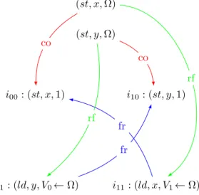
For example, if we consider the link RF( (st, y, Ω), (ld, y, V0← Ω) ), since
CO indicates that (st, y, 1) is executed after (st, y, Ω), and (ld, y, V0← Ω) reads
from this second write, we know that (st, y, 1) is executed after (ld, y, V0← Ω).
So we have FR((ld, y, V0← Ω), (st, y, 1)).
Since relation PO is defined by the program and FR is derived from CO and RF, a candidate execution can be defined by a combination of CO and RF. In other words, it is determined by a combination of permutations of store instructions to each memory location and a choice of store instruction for each load instruction. Therefore, Figure 5 is an example of a candidate execution. Another one is given page 20 by Figure 15.
5. Generic Model
In this section, we present the weakest memory model we consider, referred to as generic model. This model accepts every candidate execution as an allowed execution. The generic model allows us to produce all candidate executions by only guaranteeing that:
• for every memory location, its value is initially undefined,
• two writes at the same location cannot happen at the same time, and are ordered,
• if a store instruction is associated to a load instruction by RF, the read value is equal to the written value.
After the generation of candidate executions, forbidden executions will be fil-tered out by specific memory models (as described in Section 6).
The generation is illustrated by Figure 6 and contains the following main steps:
• adding unique identifiers to instructions (line 2), • extracting PO (line 3),
• searching address and data dependencies (line 5–6),
• extracting load and store instructions for each memory location (lines 8– 9),
• generating CO by creating a permutation of store instructions to each memory location and combining them (lines 10–11),
• generating RF by associating a store instruction to each load instruction (line 12).
During this generation, the FR relation, and the transitive closures of PO and CO are deduced using CHR rules that are activated on the fly as constraints are added into the store. The rules that are specific to each model are also activated this way. It allows MMFilter to early identify subsets of executions as forbidden by the memory model, avoiding to generate them entirely.
5.1. Extraction of PO and Dependencies
First, we add some information to instructions: a thread identifierN_thand an instruction identifierN_instinside the thread. Instructions are immediately added to the store of constraints as we process a list of instructions.
Memory operations (OP,Loc,Val) are modeled by CHR constraints of the form i(N_th, N_inst, OP, Loc, Val). Fence instructions f(t_op1, t_op2) are
modeled by CHR constraints fence(N_th, N_inst, t_op1, t_op2). For
exam-ple, instructions of the programprogram_p0in Figure 1 are translated into the following CHR constraints: i(0,0,st,x,1), i(0,1,ld,y,R0), i(1,0,st,y,1)and
i(1,1,ld,x,R1).
We also replace read-modify-write operations by a read iread followed by
a write iwrite, however in order to guarantee atomicity, we also add a CHR
constraintrmw(iread, iwrite) that is exploited by a CHR rule (presented in
Sec-tion 5.3) that rejects execuSec-tions violating atomicity of the instrucSec-tion.
The Prolog predicate enrich_prog(0,THREADS,EnrichedThreads) in Figure 6 produces the translation from original instructions to “identified” ones in a very straightforward way: it visits the different lists of instructions of the program. Then the resulting program is scanned to build the PO constraints between successive (identified) instructions.
Inside a thread, besides the PO-relation, we also need to extract two de-pendencies: data and address dependencies (produced by the Prolog predicate
compute_rel_all_threads, respectively parameterized with data and addr). A
v that is then used by i2. If i2 is a store instruction writing a value that
de-pends on v, we have a data-dependencydata(i1, i2). If i2is a memory operation
with an access to an address that depends on v, we have an address-dependency
addr(i1, i2).
The program in Figure 4 contains an address-dependency, so we produce a constraint addr( (1,0,ld,y,r11:V1) , (1,1,ld,r11:V1,r12:V2) ). If T1 had a
third instruction(st, z, r12:V2)writing the read value at some locationz, we
would have a data-dependencydata( (1,1,ld,r11:V1,r12:V2) , (1,2,st,z,r12:V2) ).
5.2. Generation of CO and RF
The production of a candidate execution can be split into two phases (cf. lines 10–12 in Figure 6): first, build a permutation of the store instructions (to produce CO); second, for each of these permutations, associate to each load instruction a possible store instruction having written the read memory location (to produce RF).
CO is a relation that orders the store instructions for each memory location. In order to produce a candidate permutation for this relation, we first find all store instructions to each location. A candidate execution is obtained by taking a permutation of store instructions to each location. For each of these permutations, we also add, at the beginning of the list, a store instruction
i(-1,-1,st,LOC,undefined)that defines the value at the given locationLOCto be
undefined before any other store instruction. The corresponding CO constraints are extracted similarly to the extraction of PO.
Extracting RF constraints requires to have both load and store instructions to each memory location. A combination of pairs load/store instructions is added to a generated set of CO constraints. For any correct access, we generate a constraintrf(i(T1,N1,st,Loc,Val), i(T2,N2,ld,Loc,Val)). Note that, as we can add a register indication inLoc and Val, the generated constraint can be slightly different, but this notation gives the general idea.
If a load instruction is performed from anundefinedmemory location a con-straintrf(undefined, Load)is generated, and reads the valueundefined. Later, a CHR rule will also produce a corresponding rte (runtime-error) constraint which means that the execution comprises an undefined memory access.
5.3. Derivation of IPO, FR and RMW Atomicity
We derive FR (the from-read relation) and IPO (the transitive closure of PO) from previously described constraints.
The FR relation associates to each load instruction, the consecutive store instructions that will, according to CO, overwrite the location the load instruc-tion reads. We implement it using two CHR rules meninstruc-tioned on the right side of Figure 7.
The first expresses that if a load instruction LD reads a value written by a store instructionSTand, according to CO, the store instruction ST1overwrites the read value, then we have a FR constraint betweenLDandST1. It corresponds, in the example of execution on the left side of the figure, to the detection of the FR constraint numbered 1.
(st, l, v) (ld, l, v) (st, l, v1) (st, l, v2) rf co co fr(1) fr(2) 1 rf ( ST , LD ) , co ( ST , ST1 ) == > fr ( LD , ST1 ). 2 fr ( LD , ST ) , co ( ST , ST2 ) == > fr ( LD , ST2 ).
Figure 7: FR computation (part of generic model.pl)
1 % PO t r a n s i t i v e c l o s u r e
2 d u p l i c a t e _ r e m o v a l @ ipo ( I0 , I1 ) \ ipo ( I0 , I1 ) <= > t r u e . 3 r e n a m e _ p o @ po ( I0 , I1 ) == > ipo ( I0 , I1 ).
4 t r a n s i t i v e _ c l o s u r e @ ipo ( I0 , I1 ) , ipo ( I1 , I2 ) == > ipo ( I0 , I2 ).
Figure 8: IPO computation rules (part of generic model.pl)
The second rule produces successive FR constraints starting from a previ-ously computed FR constraint. IfST is a instruction store that overwrites the value read byLD and, according to CO,ST2overwrites the value written byST, then we also have an FR constraint betweenLDandST2. It corresponds, in the execution on the left side of the figure, to the detection of the FR constraint numbered 2.
We define IPO as the transitive closure of PO, which is needed to define some memory models. We know that this relation is acyclic by definition. We produce IPO thanks to the rules illustrated in Figure 8. For each existing PO constraint between two instructions, we create a new constraint IPO (line 3). We then apply the transitivity using the rule in line 4. We delete duplicates as soon as possible using the rule defined in line 2.
Finally, once we know RF, CO and FR, we can add the CHR rules that guarantee the atomicity of RMW, composed of a load instruction followed by a store instruction at the same memory location. We must ensure that another store instruction cannot overwrite the value read by the load instruction of the read-modify-write operation before its store instruction is performed. We express this condition by the rule in line 1 of Figure 9. Behaviors forbidden by this rule are illustrated in Figure 10.
1 rmw ( LD , ST ) , fr ( LD , CST ) , co ( CST , ST ) <= > false .
Figure 9: RMW coherency rule (part of generic model.pl)
(ld, l, v1) (st, l, v2) (st, l, v1) (st, l, x) rmw rf fr co co
Figure 10: RMW Atomicity: forbidden scenarios
5.4. Derivation of Barrier Constraints
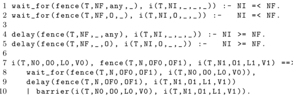
Barriers force an ordering of instructions inside a thread. The developer (or eventually the compiler) puts such barriers into the code to ensure that some operations will be effectively ordered in a certain way during execution. Depending on the hardware architecture, barriers can be more or less precise, for example by taking into account the type of operations to determine whether they can be reordered through barriers. This is why in our language, barriers require two parameters that are types of access to the memory: f(t1,t2). All operations of typet1that precede the barrier will be ordered strictly before all operations of typet2that follow the barrier.
We encode this behavior by deriving more information from constraints al-ready added to the store of constraints, namely enriched instructions, as illus-trated by Figure 11.
The predicatewait_for(resp.,delay) expresses that a barrier must wait for
an execution (resp., delay a too early execution) of an instruction of a certain type if this instruction must be ordered before (resp., after) a barrier in a given thread.
The CHR rule, lines 7 to 10, determines for a given pair of memory operations and a given barrier, if the considered memory operations are ordered by the barrier. We must check that the first instruction must be executed before the barrier, that delays the execution of the second instruction. In this case, we add
1 w a i t _ f o r ( fence (T , NF , any , _ ) , i (T , NI ,_ ,_ , _ )) : - NI = < NF . 2 w a i t _ f o r ( fence (T , NF ,O , _ ) , i (T , NI ,O ,_ , _ )) : - NI = < NF . 3
4 delay ( fence (T , NF ,_ , any ) , i (T , NI ,_ ,_ , _ )) : - NI >= NF . 5 delay ( fence (T , NF ,_ , O ) , i (T , NI ,O ,_ , _ )) : - NI >= NF . 6
7 i (T , N0 , O0 , L0 , V0 ) , fence (T ,N , OF0 , OF1 ) , i (T , N1 , O1 , L1 , V1 ) == > 8 w a i t _ f o r ( f e n c e ( T , N , OF0 , OF1 ) , i ( T , N0 , O0 , L0 , V0 )) ,
9 d e l a y ( f e n c e ( T , N , OF0 , OF1 ) , i ( T , N1 , O1 , L1 , V1 )) 10 | b a r r i e r ( i ( T , N0 , O0 , L0 , V0 ) , i ( T , N1 , O1 , L1 , V1 )).
Figure 11: Barriers computation (part of generic model.pl)
a new CHR constraintbarrier/2for these instructions into the store.
6. Specific Models
The generic model allows to produce all candidate executions of a program by considering a very weak memory model. An execution is defined by a com-bination of CO and RF. Other relations, like the program order PO or address and data dependencies are not necessary to characterize a candidate execution. To describe a specific memory model, the principle is to define the relations that must be respected in order to accept a candidate execution as an allowed execution. A model M respects (i.e. preserves) a relation R if any pair of instructions ordered by R is guaranteed to happen in the corresponding order in the executions allowed by M .
In order to define the relation respected by a specific model, we define a new CHR constraint R, that will be named after the considered memory model (sc(I0,I1) for SC, tso(I0,I1) for TSO, ...). This constraint is defined as a union of relations that the model guarantees to respect. For each candidate execution, we build the transitive closure of this new constraint. If it exhibits a cycle, meaning that an operation happens before itself (which is inconsistent), the execution is forbidden. Otherwise, it is allowed.
6.1. Cycle Detection
For a given memory model, let R denote the relation that the model has to respect for memory operations in an execution. R is defined as the union of subsets of basic relations of the generic model. For example, SC will completely respect PO, CO, RF and FR. On the other hand, a model like TSO will re-spect only a subset of PO. Once we know R, we get a way to determine which instructions must (transitively) happen before another one. To detect an in-consistent execution, we explore the lists of constraints between instructions. If these lists exhibit a cycle, it means that according to the model, an instruction must happen before itself, which is inconsistent.
1 rel (R , Begin , End ) \ rel (R , Begin , End ) <= > true . 2 path (R , Begin , End ) \ path (R , Begin , End ) <= > true .
3 path (R , Begin , End ) , rel (R , End , Begin ) == > cycle (R , Begin ). 4
5 rel (R , Begin , End ) == > inf ( Begin , End ) | path (R , Begin , End ). 6 path (R , Begin , End ) , rel (R , End , Next ) == >
7 inf ( Begin , N e x t ) | p a t h ( R , Begin , N e x t ).
Figure 12: Cycle detection (cycle.pl)
This cycle detection is produced using CHR constraints parameterized by the relation R. Contrary to the computation of IPO previously mentioned, the closure can now exhibit cycles, which have to be correctly detected to ensure termination. Detection rules are illustrated by Figure 12.
We use three CHR constraints declared at line 1 of the figure. The con-straintrel(R,Begin,End)indicates that instructions Begin andEnd are ordered
byR. This representation of R(Begin,End)allows to make the cycle detection
generic. The transitive closure of R is progressively computed using a constraint
path(R,Begin,End), which means that there exists a path betweenBeginandEnd
(End 6= Begin) composed of edges in R. Finally the constraintcycle(R,Begin)
indicates that starting from the instructionBegin, we found a non trivial path of constraintsRreturning to this instruction.
Then, we define the rules that will propagate the constraints ensured by the model. We also add some rules of simplification and simpagation that will limit the quantity of generated traces, deleting duplicates and stopping propagation on traces that have already exhibited a cycle.
The first rules (lines 3 and 4) allow to avoid the explosion of the number of traces. The first rule of simpagation removes duplicates of the relation R. Using the same pattern, the rule in line 4 removes paths that have the same beginning and end. Indeed, if there exists two paths, even different, from an instruction i1to an instruction i2, it is not useful to keep this distinction for the
cycle detection. If there exists a cycle using one path, it trivially follows that there exists another cycle using the other path. This is why we do not need to keep the entire path inside the CHR constraintpath.
The propagation rule at line 5 allows, when we detect a path and an R constraint that closes this path, to create a new constraint indicating a cycle. Inside the definition of a model, we add a CHR rule that introduces false
into the store of constraints if a cycle is detected, which allows to stop the propagation. Indeed, we usually only want to keep allowed executions. Without this rule, the tool will output all candidate executions, where forbidden ones reach a store of constraints that contains a cycle.
The next rules are used to propagate path relation between instructions. The rule on line 8–9 allows to add a new path every time we find a constraint that makes an existing path grow. In order to optimize the search of paths and to avoid detecting the same cycle several times, we suppose an arbitrary total
1 2 3 4 5 r r r r r
Figure 13: Example of graph: a “6” configuration.
order relation over instructions, and denote the fact that instructioni1is strictly inferior toi2with respect to this relation by the Prolog predicateinf(i1,i2). For example, such a total order relation can be defined as a lexicographic order on the pairs (thread identifier, instruction identifier). This optimization consists in adding a new edge in the end of the path only if, according toinf, the new end node is strictly greater than the beginning of the path. Note that we compute cycles from all instructions at the same time. By using this optimization, we only consider paths whose origin is strictly inferior to next instructions. Indeed, we only need to consider cycles that do not pass multiple times by the same element. Consequently, we only need to start from the minimal instruction (according to
inf) since in such a cycle, there exists an instruction that is strictly inferior to any other.
The creation of the beginning of a path (rule on line 7) is allowed under the same condition. We start a new path only if its origin is inferior to the following instruction. The soundness of this optimization will be discussed in Section 7.
Consider the graph in the form of a “6” in Figure 13, where we simply use numbers to label nodes and define the relation r. We assume thatinf(Begin, End)
is defined by an integer comparisonBegin < End. Let us apply the rules of Fig-ure 12 on a set of constraints that define the graph:
?- rel(r,5,2), rel(r,2,4), rel(r,4,3), rel(r,1,2), rel(r,3,5). First, the constraint rel(r,5,2) is added to the store. No rules can be activated by this constraint (since the guard 5 < 2 of the rule on line 7 of Figure 12 that creates a path is not valid):
STORE={ rel(r,5,2) }
Adding the constraint rel(r,2,4)activates the propagation rule (line 7 in Figure 12) that starts a new path and produces a path constraintpath(r,2,4). We cannot continue this path at the moment, so we do not perform other actions: STORE={ rel(r,5,2),
rel(r,2,4),path(r,2,4) }
Adding rel(r,4,3)does not create a new path departure since 4 ≥ 3, but it can make grow the pathpath(r,2,4)since 2 < 3. Thus the rule on line 5 in Figure 12 adds a new constraintpath(r,2,3).
STORE={ rel(r,5,2),
rel(r,2,4),path(r,2,4), rel(r,4,3),path(r,2,3) }
Then, the solver adds the constraintrel(r,1,2). It adds a new pathpath(r,1,2)
that can be extended withrel(r,2,4), adding the constraintpath(r,1,4), that can in turn be extended withrel(r,4,3), creating path(r,1,3). Note that the guards are satisfied since 1 < 2, 1 < 4 and 1 < 3 (cf. lines 7–9 in Figure 12). STORE={ rel(r,5,2),
rel(r,2,4),path(r,2,4), rel(r,4,3),path(r,2,3),
rel(r,1,2),path(r,1,2),path(r,1,4),path(r,1,3) }
The solver finally adds the last constraintrel(r,3,5). It leads to a new path
path(r,3,5), bringing us to the store: STORE={ rel(r,5,2),
rel(r,2,4),path(r,2,4), rel(r,4,3),path(r,2,3),
rel(r,1,2),path(r,1,2),path(r,1,4),path(r,1,3), rel(r,3,5),path(r,3,5) }
The constraintrel(r,3,5)has already been used to activate the rule of path creation. It can now be used to extend existing paths. In the store, we have two paths that can be extended with this constraint: path(r,2,3)andpath(r,1,3). The refined semantics does not give priority to one of them.
If path(r,2,3) is chosen, we create path(r,2,5), which is then used with
rel(r,5,2)to activate the cycle detection, and the algorithm terminates. Ifpath(r,1,3)is chosen, first we createpath(r,1,5), which is now used with
rel(r,5,2)to create a constraintpath(r,1,2). The store becomes: STORE={ rel(r,5,2), rel(r,2,4),path(r,2,4), rel(r,4,3),path(r,2,3), rel(r,1,2),path(r,1,2),path(r,1,4),path(r,1,3), rel(r,3,5),path(r,3,5), path(r,1,5),path(r,1,2) }
Aspath(r,1,2)already exists, the rule of duplicate removal is activated. In most CHR implementations (including SWI-Prolog, that we use), the oldest added constraint will be kept, removing the newest (we will detail this in Section 7). As a result, the new constraintpath(r,1,2)is immediately removed from the store, and for the choice path(r,1,3), the propagation stops, giving the possibility to the solver to explore thepath(r,2,3)constraint as previously detailed (and terminating with the detection of the cycle).
1 : - i n c l u d e ( g e n e r i c _ m o d e l ). 2 : - i n c l u d e ( cycle ).
3
4 % SC does not c o n s i d e r any fences 5 fence (_ ,_ ,_ , _ ) <= > true . 6 % Nor a d d r e s s / data d e p e n d e n c y 7 addr (_ , _ ) <= > true . 8 data (_ , _ ) <= > true . 9 10 % If we d i s c o v e r a cycle in SC , it is an i n c o h e r e n c y 11 cycle ( sc , L ) <= > false . 12 13 po ( I0 , I1 ) == > rel ( sc , I0 , I1 ). 14 co ( I0 , I1 ) == > rel ( sc , I0 , I1 ). 15 rf ( I0 , I1 ) == > rel ( sc , I0 , I1 ). 16 fr ( I0 , I1 ) == > rel ( sc , I0 , I1 ). Figure 14: SC Model (sc.pl) 6.2. SC Memory Model
The sequentially consistent memory model is the strongest model. This is also the easiest to implement with our constraints as we only have to say that this model respects PO, CO, RF and FR relations. This model is illustrated in Figure 14. The includes in lines 1 and 2 respectively add the definition of the generic model and the rules for cycle detection.
For each constraint PO, CO, RF or FR we meet, we add a new constraint
rel/2 corresponding to the SC relation (lines 13–16). Cycle detection rules will use these constraints to search for cycles in the transitive closure of the relations guaranteed to be respected by SC. As we previously mentioned, we add a simplification rule (line 11) that introduces falsein the store of constraints whenever a cycle is detected. It is used to early prune the search tree.
We can notice that, as the SC memory model respects PO, barriers and data or address dependencies do not bring new information about the order of execution of instructions. That is why we remove them using simplification rules (lines 5,7,8), allowing to limit the quantity of redundant constraints in the store2.
For example, this model detects that the undesirable behavior of the pro-gram p0 of Figure 1 that allows both threads to read Ω is forbidden by SC, as
illustrated by Figure 15. The execution exhibits a cycle i00, i01, i10, i11, i00, since
PO and FR must be respected by SC.
2This choice, where we add and then explicitly remove constraints, allows to ease the
i01: (ld, y, V0← Ω) i11: (ld, x, V1← Ω) i00: (st, x, 1) i10: (st, y, 1) (st, y, Ω) (st, x, Ω) po po co co rf rf fr fr
Figure 15: Execution forbidden by the SC model for program p0 of Figure 1
6.3. SC per Location
Let us now focus on weaker models, like those of widespread processor archi-tectures. A first relation, that exists in most architectures [2], ensures a basic coherency of code execution on a single ship.
It consists in ensuring, for each core, the coherency of memory accesses to each memory location [10] (the correct serialization of store instructions to a memory location). If a core stores v at a location l and then reads v0 at l, then corresponding stores w and w0must be realized in this order: w0cannot happen before w. Following the formalization of [6], we name this relationsc_per_loc/2. The verification of its coherency also consists in verifying the absence of cycles in the relation.
We provide the definition of the corresponding coherency rules in Figure 16. The relationsc_per_loc is defined as the union of CO, RF, FR and po_loc/2
(lines 13–16). Thepo_loc relation (lines 10–11) corresponds to the order PO,
but restricted to the operations happening to a same memory location. We build it using IPO (the transitive closure of PO). The mono-processor coherency requires thatsc_per_locshould be acyclic.
As we did for the definition of SC, we define an execution with a cycle as a rejected execution (line 8).
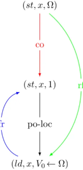
For example, we can consider a sequential program that first writes the value 1 at a memory location x and then reads it. The SC per location relation ensures that we cannot read the initial value, as illustrated by Figure 17.
We will use this relation as a necessary starting point for every memory model defined in the next sections.
1 : - u s e _ m o d u l e ( l i b r a r y ( chr )). 2 : - i n c l u d e ( cycle ).
3 : - c h r _ c o n s t r a i n t po_loc /2. 4
5 % U n i p r o c Check : sc per location , a c y c l i c i t y of
6 % co ∪ rf ∪ fr ∪ p o _ l o c
7
8 cycle ( sc_per_loc , L ) <= > false . 9
10 ipo ( i ( N0 , Id0 , O0 ,L , V0 ) , i ( N1 , Id1 , O1 ,L , V1 )) == > 11 p o _ l o c ( i ( N0 , Id0 , O0 , L , V0 ) , i ( N1 , Id1 , O1 , L , V1 )). 12
13 co ( I0 , I1 ) == > rel ( s c _ p e r _ l o c , I0 , I1 ). 14 rf ( I0 , I1 ) == > rel ( s c _ p e r _ l o c , I0 , I1 ). 15 fr ( I0 , I1 ) == > rel ( s c _ p e r _ l o c , I0 , I1 ). 16 po_loc ( I0 , I1 ) == > rel ( sc_per_loc , I0 , I1 ).
Figure 16: SC per Location model (uniproc.pl)
(ld, x, V0← Ω) (st, x, 1) (st, x, Ω) po-loc co rf fr
Figure 17: Execution forbidden by sc per loc relation when we read a value previously written by the same thread
6.4. TSO and PSO Memory Models
TSO and PSO memory models relax the program order PO for pairs of instructions that start with a store operation. PSO is weaker than TSO since TSO relaxes store-load pairs whereas PSO relaxes all pairs starting with a store instruction. The relation is transitively relaxed, so we build these models using IPO, as illustrated for TSO in Figure 18 (line 15-16). The idea is that any created pair preserved program-order (ppo/2) starting with a store instruction and ending with a load instruction must be immediately removed since this order is not respected by the model.
To obtain PSO, in order to remove any pair starting with a store instruction, we need to replace the line 15 withppo(i(_,_,st,_,_),_) <=> true.
Following [6], we add the reads-from external (rfe/2) relation. Indeed, store instructions performed by a core use an internal store-buffer. If the core asks for a value at a location where it has stored a value recently, this buffer is also a cache. Consequently, such a load instruction cannot be seen by other cores, and we must not take it into account in the global order of operations [2]. This relation is created using a Prolog predicate and a guarded CHR rule (lines 9– 10). Two operations are related by an external RF relation if they are related by RF and they are not performed by the same thread (line 9 in Figure 18). There exists an rfe(reads-from external) constraint between two instructions, if there exists an rf constraint between them and if these instructions satisfy the predicateextthat checks that they have different thread identifiers.
TSO and PSO respect the SC per location relation, so we include this part of the model in line 1. In these models, barriers are strong so we treat all of them the same way: we restore PO each time two instructions are ordered by a barrier (line 18).
Under TSO, the execution of the program p0forbidden by SC (cf. Figure 15)
is allowed since thepo constraints that close the cycle are not kept by TSO,
as illustrated by Figure 19. The program p1 forbids the execution by adding
fences, and we get back the cycle (i00, i01, i10, i11, i00) that forbids the execution
(Figure 20).
7. Termination of the Analysis
This section gives the main principles that ensure the termination of the different parts of the analysis of a program:
• generation of candidate executions, • deduction of derived relations,
• cycle detection for the relations defined by the model. Each of these steps must terminate to ensure global termination.
1 : - i n c l u d e ( u n i p r o c ). 2 : - c h r _ c o n s t r a i n t rfe /2. 3 : - c h r _ c o n s t r a i n t ppo /2. 4
5 % TSO i m p l e m e n t a t i o n does not need addr and data deps : 6 addr (_ , _ ) <= > true . 7 data (_ , _ ) <= > true . 8 9 ext ( i ( N0 ,_ ,_ ,_ , _ ) , i ( N1 ,_ ,_ ,_ , _ )) : - \+ N0 = N1 . 10 rf ( I0 , I1 ) == > ext ( I0 , I1 ) | rfe ( I0 , I1 ). 11
12 cycle ( tso , L ) <= > false . 13
14 % po - WR pairs are not p r e s e r v e d by TSO , so we remove them 15 ppo ( i (_ ,_ , st ,_ , _ ) , i (_ ,_ , ld ,_ , _ )) <= > true .
16 ipo ( I0 , I1 ) == > ppo ( I0 , I1 ). 17
18 b a r r ie r ( I0 , I1 ) == > rel ( tso , I0 , I1 ). 19 ppo ( I0 , I1 ) == > rel ( tso , I0 , I1 ). 20 rfe ( I0 , I1 ) == > rel ( tso , I0 , I1 ). 21 co ( I0 , I1 ) == > rel ( tso , I0 , I1 ). 22 fr ( I0 , I1 ) == > rel ( tso , I0 , I1 ).
Figure 18: TSO memory model (tso.pl)
i01: (ld, y, V0← Ω) i11: (ld, x, V1← Ω) i00: (st, x, 1) i10: (st, y, 1) (st, y, Ω) (st, x, Ω) co co rf rf fr fr
i01: (ld, y, V0← Ω) i11: (ld, x, V1← Ω) i00: (st, x, 1) i10: (st, y, 1) (st, y, Ω) (st, x, Ω) barrier barrier co co rf rf fr fr
Figure 20: In p1, the undesirable execution (cf. Figure 15) is forbidden by TSO
7.1. Generation of Candidate Executions
Figure 6 shows the predicate that produces the generation of candidate ex-ecutions. The predicate enrich_prog (line 2) consists in a simple visit of the instructions in order to modify them. We have a finite number of threads and a finite number of instructions per thread, so the execution terminates. The termination of compute_pos (line 3) and compute_rel_all_threads (lines 5–6) is justified in the same way. For the last one however, we must consider all instructions that follow every given instruction.
The termination ofops_to_each(lines 8–9) is partially ensured by the afore-mentioned ideas, but here, we also possibly have backtracking if the accessed memory location is a Prolog variable. For each memory access, these backtrack-ings are limited by the number of memory locations (comprising the variables ofVARSandundefined), so we only generate a finite number of branches.
The generated STORES and LOADS are lists of finite lists of instructions. It
follows that permute_stores (line 10) andcompute_all_rfs (lines 12) will gen-erate a limited amount of permutations when they backtrack. The predicate
compute_all_cos(line 11) visits the generated finite list PSTORES, allowing ter-mination.
7.2. Derivation of Relations
The construction of relations derived from the basic relations of a given candidate execution can belong to one of two categories:
• renaming of an existing relation,
The first category is employed for the definition of new memory models. These are the rules that we can for example see on lines 13–16 in Figure 14, where we rename po(I0, I1)as rel(sc,I0,I1), and similarly for CO, RF and FR. These rules trivially terminate since any CHR constraint can activate such a renaming rule only once. It is, of course, assumed that the model generates only a finite number of basic relations.
The second category is used to derive, from the original relations of a given candidate execution, new relations that are acyclic. This is for example the case for IPO, the transitive closure of PO (Figure 8) that is guaranteed to be acyclic. This is also the case for the FR relation shown in Figure 7, where the rule on line 1 can be applied for a finite number of combinations of the initial CO and RF constraints, while the rule on line 2 is applied a finite number of times since CO constraints do not comprise cycles and thus the number of successive store instructions after each given store instruction is also finite. Therefore, the computation terminates.
7.3. Cycle Detection
The CHR rules we use to detect cycles (cf. Figure 12) is a variant of the ones defined by Fr¨uhwirth in [14] for the computation of the transitive closure of a relation in a graph, that we optimized for our problem. In our case, we aim at finding cycles and not computing the entire transitive closure if we can avoid it. We stop when we find a cycle and, since we add constraints as we generate relations for the execution we are treating, we can detect a cycle before having generated the entire set of constraints that corresponds to an execution. Note however that if the execution does not exhibit cycles, the entire closure is computed. We also limit the search space using an arbitrary orderinf defined in Section 6.
The termination of the rules proposed by Fr¨uhwirth relies on two main as-sumptions about the underlying CHR implementation. First, it must respect the refined semantics [13] that orders the activation of the rules (using their definition order). Second, the simpagation rules must always try to remove the constraints that have been added the most recently into the store. It avoids for a new constraint c duplicating c0 to propagate all information that has already been propagated for c. These two assumptions are respected by most CHR implementations including SWI-Prolog.
The rules proposed by Fr¨uhwirth are the following:
1 p a t h ( Begin , End ) \ p a t h ( Begin , End ) <= > t r u e .
2 e d g e ( Begin , End ) == > p a t h ( Begin , End ).
3 p a t h ( Begin , End ) , e d g e ( End , N e x t ) == > p a t h ( Begin , N e x t ). Fr¨uhwirth [14, Sec.2.4.1] justifies that this program is terminating. Intuitively, in this version, if we have a non-trivial cyclen1,n2, . . . ,nk,n1(where alln1, . . . ,nk
are different), we will build constraintspath(n1,n2), . . . ,path(n1,nk),path(n1,n1),
and finally add path(n1,n2)again. As the implementation follows the refined
1 ppo ( i (_ ,_ , st ,_ , _ ) , i (_ ,_ , ld ,_ , _ )) <= > true . 2 ipo ( I0 , I1 ) == > ppo ( I0 , I1 ). Selective removal 1 ipo ( i (N ,T , ld ,L , V ) , I1 ) == > 2 ppo ( i ( N , T , ld , L , V ) , I1 ). 3 ipo ( i ( N0 , T0 , st , L0 , V0 ) , i ( N1 , T1 , st , L1 , V1 )) == > 4 ppo ( i ( N0 , T0 , ld , L0 , V0 ) , i ( N1 , T1 , st , L1 , V1 )). Selective addition
Figure 21: Two ways to define the subset of a relation
constraintpath(n1,n2)and keep the older one, which cannot be used again to extend the path along the cycle.
Our optimization consists in:
• adding guards to the rules that add new constraintspath, • adding a rule to detect cycles.
The guards obviously do not disrupt termination, they only limit the quan-tity of paths created at the beginning of the search and the possibilities of path extension. If the extension of a path that contains a cycle, is allowed by the guard, guards never prevent the removal of the generated duplicate constraint since the rule of duplicate removal is applied before extending it again.
The cycle detection rule does not prevent the algorithm from terminating neither. It only adds a new constraint when a new cycle is found.
8. Evaluation
In this section, we further discuss the soundness of MMFilter and provide an experimental evaluation of its soundness and performances.
8.1. Correct Constraint Removal
If a relation is only partially preserved by a model, some of the corresponding constraints must not be considered by the cycle detection. For example, for the TSO and PSO memory models, we defined a new relation “preserved program-order” which is a subset of “program-program-order”. Such a subset can be built in two different ways: either we only add constraints that must be considered, or we add all of them and remove on-the-fly those we do not want to consider. We illustrate these different ways with the definition of ppo for TSO in Figure 21. The first one adds all constraints, removing those of the form ppo(st,ld), while the second one only adds the constraints ppo(st,st) and ppo(ld,any).
It is important to ensure that a constraint that must be removed is never used by a derivation rule of the model (or the cycle detection) before it is
1 mp3t3 (V , [ T0 , T1 , T2 ]) : -2 V = [ x , m ] , 3 T0 = [( st , x ,10) ,( st , m ,1) , ( ld , m , M2 ) ,( ld , x , X2 )] , 4 T1 = [( ld , m , M0 ) ,( ld , x , X0 ) ,( st , x ,20) ,( st , m ,2) ] , 5 T2 = [( ld , m , M1 ) ,( ld , x , X1 ) ,( st , x ,30) ,( st , m ,3) ]. 6 7 m p 4 t 4x 1 (V , [ T0 , T1 , T2 , T3 ]) : -8 V = [ x , m ] , 9 T0 = [( st , x ,10) ,( st , m ,1) ,( ld , m , M3 ) ,( ld , x , X3 )] , 10 T1 = [( ld , m , M0 ) ,( ld , x , X0 ) ,( st , x ,20) ,( st , m ,2) ] , 11 T2 = [( ld , m , M1 ) ,( ld , x , X1 ) ,( st , x ,30) ,( st , m ,3) ]. 12 T3 = [( ld , m , M2 ) ,( ld , x , X2 ) ,( st , x ,40) ,( st , m ,4) ].
Figure 22: Message passing examples MP3 and MP4
removed. As we use the refined semantics of CHR, rules are applied in their order of definition. More particularly, when a constraint is added, we have the guarantee that the rules that can be activated will be applied in the order of the CHR program. Consequently, a removal rule for a constraint T must be ordered before any rule that can be activated by T . It ensures that the removal rule will be first activated, and if the constraint must be removed, it will be done before it could activate any other rule. In the models we defined, it is the case.
8.2. Testing and Performances
Our goal was to evaluate the following research questions: (RQ1) Do Herd and MMFilter produce the same results ?
(RQ2) What are the performances of MMFilter compared to Herd ?
For the experimental evaluation of MMFilter, we used program samples from the test suite of Herd in order to have an oracle. These examples can be found on the Herd tool webpage at http://virginia.cs.ucl.ac.uk/herd/ (record “armed cats”).
Regarding (RQ1), on all tested examples, MMFilter produced the same re-sults as Herd, providing a cross validation of both tools. Our models being based on those of Herd, our goal is not to verify them but to verify the validity of the underlying generic solver.
Regarding (RQ2), the execution of MMFilter on these small examples is very fast and does not allow to precisely evaluate its performances. We created some additional examples that contain more instructions in order to bring the solvers to more complex solving tasks. We compare MMFilter running over SWI-Prolog 7.7.4 with Herd 7.47. The hardware used for experiments comprises an Intel Core i7-6700HQ, 4 physical cores, 2.6GHz, with 16GB of RAM.
Figure 22 presents two examples of some (potentially wrong) message pass-ing, with 3 and 4 threads (and accordingly, 3 and 4 messages). Each thread
1 mp3t2 (V , [ T0 , T1 ]) : -2 V = [ x , m ] , 3 T0 = [( st , x ,10) ,( st , m ,1) ,( ld , m , M2 ) ,( ld , x , X2 ) , 4 ( st , x ,30) ,( st , m ,3)] , % s e n d one m o r e 5 T1 = [( ld , m , M0 ) ,( ld , x , X0 ) ,( st , x ,20) ,( st , m ,2) , 6 ( ld , m , M1 ) ,( ld , x , X1 )]. % r e c e i v e one m o r e 7 8 m p 4 t 4x 4 (V , [ T0 , T1 , T2 , T3 ]) : -9 V = [ x0 , x1 , x2 , x3 , m ] , % now 4 x ’ s 10 T0 = [( st , x0 ,10) ,( st , m ,1) ,( ld , m , M3 ) ,( ld , x3 , X3 )] , 11 T1 = [( ld , m , M0 ) ,( ld , x0 , X0 ) ,( st , x1 ,20) ,( st , m ,2) ] , 12 T2 = [( ld , m , M1 ) ,( ld , x1 , X1 ) ,( st , x2 ,30) ,( st , m ,3) ] , 13 T3 = [( ld , m , M2 ) ,( ld , x2 , X2 ) ,( st , x3 ,40) ,( st , m ,4) ]. 14 15 m p 4 t 4 x 1 _ f o r c e d _ 4 (V , [ T0 , T1 , T2 , T3 ]) : -16 V = [ x , m ] , 17 % We c o n s t r a i n r e a d v a l u e s M0 ,... , M3 18 M0 = 1 , M1 = 2 , M2 = 3 , M3 = 4 , 19 T0 = [( st , x ,10) ,( st , m ,1) ,( ld , m , M3 ) ,( ld , x , X3 )] , 20 T1 = [( ld , m , M0 ) ,( ld , x , X0 ) ,( st , x ,20) ,( st , m ,2) ] , 21 T2 = [( ld , m , M1 ) ,( ld , x , X1 ) ,( st , x ,30) ,( st , m ,3) ] , 22 T3 = [( ld , m , M2 ) ,( ld , x , X2 ) ,( st , x ,40) ,( st , m ,4) ].
Figure 23: Variants of message passing examples MP3 and MP4
sends and receives (or conversely, receives and sends) one message containing a message identifier mand a value x. These examples are interesting for perfor-mance evaluation since the combinatorial complexity is high: they successively store at several locations (thus, there are a lot of permutations of CO to gener-ate) and read the same locations.
In order to measure the impact of the number of threads, we have written variants of these examples with the same number of messages handled by less threads. For instance, for themp3t3example, the variantmp3t2 (cf. Figure 23) has only two threads, whereT0(resp.,T1) sends (resp., receives) two messages instead of one. Similarly, we have built variants ofmp4t4x1with 3 and 2 threads. We have also studied some variants of mp4t4x1 with 2, 3, or 4 instances of the variable x to measure the impact of the number of variables. Figure 23 illustrates the variantmp4t4x4with 4 variables. Note that we have also studied equivalent variants formp3t3that we do not discuss here since they are executed very fast by both MMFilter and Herd and do not provide additional evidence for comparison.
Finally, we have tested the generation of executions for expected read values. For example, the programmp4t4x1_forcedillustrated in Figure 23 expects that the message passing is sequenced so that T1 (resp., T2, T3, T0) receives the message sent byT0(resp.,T1,T2,T3). Therefore, we use the Prolog variablesM0,
Example #threads Model #executions Herd MMFilter MP3 2 Generic 147 456 1.2s 3.7s PSO 188 3.8s 1.1s TSO 92 3.8s 0.7s SC 72 5.5s 0.7s 3 Generic 147 456 1.2s 3.7s PSO 2 258 3.7s 6.4s TSO 800 3.8s 3.2s SC 678 5.2s 3.3s MP4 2 Generic 225 000 000 1 405s 6 394s PSO 1 600 6 245s 25s TSO 589 6 245s 12s SC 407 > 2h 11s 3 Generic 225 000 000 1 219s 6 221s PSO 49 305 5 883s 559s TSO 11 971 5 913s 154s SC 9 123 > 2h 139s 4 Generic 225 000 000 1 206s 5 885s PSO 516 030 5 696s 2 782s TSO 96 498 5 775s 735s SC 81 882 > 2h 726s
Figure 24: Performance evaluation results for Herd and MMFilter for MP3, MP4 and their variants with a different number of threads
speedcheckthat allows to generate only executions respecting a constraint on some variables in the program. In this case, it is applied for the values read for the variablem. Again, we do not present the results for the variants of mp3t3
that are executed too fast to be relevant.
The goal is to determine all allowed executions for a given program. For each example, we analyze the program with different memory models. We indicate the number of executions allowed by the model. The number indicated for the generic model corresponds to the number of candidate executions. We set a timeout to two hours of computation.
Figure 24 illustrates the results of tests for Herd and MMFilter for the mes-sage passing on the variants having a different number of threads. We note that when the combinatorial complexity is particularly strong, MMFilter is faster, particularly when the execution is heavily constrained. The stronger the model is, the faster MMFilter runs, while Herd reacts in the opposite way. This is mainly due to the fact that Herd generates all candidate executions and en-tirely propagates the relations between the instructions, while MMFilter prunes entire execution subtrees as soon as it finds a cycle, even in an incompletely generated candidate execution. Consequently, a stronger model increases the chances to have a more aggressive pruning for MMFilter, while it requires more
#Variables x Model #executions (%) Herd MMFilter 1 Generic 225 000 000 (100.%) 1 206s 5 885s PSO 516 030 (0.23%) 5 696s 2 782s TSO 96 498 (0.04%) 5 775s 735s SC 81 882 (0.04%) > 2h 726s 2 Generic 11 520 000 (100.%) 97s 273s PSO 105 368 (0.91%) 310s 648s TSO 27 350 (0.23%) 315s 192s SC 24 842 (0.22%) 469s 166s 3 Generic 1 080 000 (100.%) 17s 25s PSO 24 684 (2.28%) 37s 109s TSO 9 036 (0.83%) 38s 50s SC 8 285 (0.77%) 50s 45s 4 Generic 240 000 (100.%) 6s 6s PSO 11 444 (4.77%) 12s 36s TSO 5 256 (2.19%) 12s 24s SC 4 893 (2.04%) 15s 22s
Figure 25: Performance evaluation results for Herd and MMFilter for MP4 and its variants with a different number of x variables
computation for Herd. On the other hand, the generation of candidate execu-tions is longer for MMFilter and faster for Herd since the corresponding model is weaker.
Similarly, for programs with less threads, there are more operations in each thread, that leads to more PO constraints (and consequently, preserved-PO) on the load and store operations. Again, it increases the chances for early pruning in MMFilter while requiring more computation for Herd.
Figure 25 illustrates the results of tests for the variants of the MP4 message passing program with different numbers of variables. Here, we can see that, compared to MMFilter, Herd behaves better as the number of variables grows. The main reason is the fact that the example with a greater number of variables has less dependencies between the read and written values: instead of having a long story about one variable, we have independent short stories about dif-ferent variables. So for a bigger number of variables, we have less constraints and, consequently, a greater rate of allowed executions with respect to the total number of candidate executions (the rate is indicated in parentheses). For ex-ample, for MP4 with one variable, the number of allowed executions for PSO is about 0.23% of the number of candidate executions, whereas it is about 4.77% with 4 variables. That means that, with a constant number of operations, the pruning in MMFilter becomes less efficient with respect to Herd as the number of variables grows. We can also notice that the number of candidate executions heavily decreases.
ConstrainedMvariables Model #executions Herd MMFilter None Generic 225 000 000 1 206s 5 885s PSO 516 030 5 696s 2 782s TSO 96 498 5 775s 735s SC 81 882 > 2h 726s M0 Generic 45 000 000 269s 1 141s PSO 158 018 1 156s 860s TSO 18 092 1 170s 162s SC 17 812 1 816s 159s M0+M1 Generic 9 000 000 78s 230s PSO 17 997 250s 121s TSO 660 252s 12s SC 658 381s 11s M0+M1+M2 Generic 1 800 000 37s 46s PSO 1 218 71s 11s TSO 10 71s 2s SC 10 97s 2s All Generic 360 000 29s 9s PSO 279 35s 4s TSO 1 36s 2s SC 1 41s 2s
Figure 26: Performance evaluation results for Herd and MMFilter for MP4 and its variants with a different number of constrained values read for the m variable
program with a different number of constrained values read fromm. Note that the choice of values being constrained can slightly affect the number of allowed executions. Here, we use one possible choice. Again, the more the executions are constrained, the faster MMFilter is compared to Herd.
To sum up, our experimental evaluation shows that MMFilter produces the same results as Herd for examples of its test suite. Regarding performances, as MMFilter is designed to immediately reject forbidden executions, it brings the benefit to early prune the search tree without completely generating each execution. This is particularly beneficial for strong memory models, for example TSO and SC, or when the executions are already constrained by other conditions (e.g. on read values or sequences of instruction in the same thread), while weaker models like PSO prevent aggressive early pruning. Herd is faster for weak models, where the early pruning cannot be really aggressive.
9. Conclusion and Future Work
We have presented MMFilter, an original CHR-based solver for detection of admissible executions of a given program with respect to a given memory model, and illustrated it for SC, TSO and PSO models. The ARM model