HAL Id: hal-01806227
https://hal.archives-ouvertes.fr/hal-01806227
Submitted on 18 Dec 2020
HAL is a multi-disciplinary open access
archive for the deposit and dissemination of
sci-entific research documents, whether they are
pub-lished or not. The documents may come from
teaching and research institutions in France or
abroad, or from public or private research centers.
L’archive ouverte pluridisciplinaire HAL, est
destinée au dépôt et à la diffusion de documents
scientifiques de niveau recherche, publiés ou non,
émanant des établissements d’enseignement et de
recherche français ou étrangers, des laboratoires
publics ou privés.
pre-industrial conditions? – a model study with a fully
coupled ice-sheet–climate model
M. Bügelmayer, Didier M. Roche, H. Renssen
To cite this version:
M. Bügelmayer, Didier M. Roche, H. Renssen. How do icebergs affect the Greenland ice sheet
un-der pre-industrial conditions? – a model study with a fully coupled ice-sheet–climate model. The
Cryosphere, Copernicus 2015, 9 (3), pp.821 - 835. �10.5194/tc-9-821-2015�. �hal-01806227�
www.the-cryosphere.net/9/821/2015/ doi:10.5194/tc-9-821-2015
© Author(s) 2015. CC Attribution 3.0 License.
How do icebergs affect the Greenland ice sheet under pre-industrial
conditions? – a model study with a fully coupled ice-sheet–climate
model
M. Bügelmayer1, D. M. Roche1,2, and H. Renssen2
1Vrije Universiteit Amsterdam, Amsterdam, the Netherlands
2Laboratoire des Sciences du Climat et de l’Environnement (LSCE), CEA/CNRS-INSU/UVSQ,
Gif-sur-Yvette CEDEX, France
Correspondence to: M. Bügelmayer (m.bugelmayer@vu.nl)
Received: 19 November 2013 – Published in The Cryosphere Discuss.: 7 January 2014 Revised: 13 January 2015 – Accepted: 9 April 2015 – Published: 4 May 2015
Abstract. Icebergs have a potential impact on climate since
they release freshwater over a widespread area and cool the ocean due to the take-up of latent heat. Yet, so far, ice-bergs have never been modelled using an ice-sheet model coupled to a global climate model. Thus, in climate mod-els their impact on climate has been restricted to the ocean. In this study, we investigate the effect of icebergs on the climate of the mid- to high latitudes and the Greenland ice sheet itself within a fully coupled ice-sheet (GReno-ble model for Ice Shelves and Land Ice, or GRISLI)–earth-system (iLOVECLIM) model set-up under pre-industrial cli-mate conditions. This set-up enables us to dynamically com-pute the calving sites as well as the ice discharge and to close the water cycle between the climate and the cryosphere model components. Further, we analyse the different impact of moving icebergs compared to releasing the ice discharge at the calving sites directly. We performed a suite of sensitivity experiments to investigate the individual role of the differ-ent factors that influence the impact of the ice release on the ocean: release of ice discharge as icebergs versus as freshwa-ter fluxes, and freshening and latent heat effects. We find that icebergs enhance the sea-ice thickness around Greenland, thereby cooling the atmosphere and increasing the Greenland ice sheet’s height. Melting the ice discharge directly at the calving sites, thereby cooling and freshening the ocean lo-cally, results in a similar ice-sheet configuration and climate as the simulation where icebergs are explicitly modelled. Yet, the simulation where the ice discharge is released into the ocean at the calving sites while taking up the latent heat ho-mogeneously underestimates the cooling effect close to the
ice-sheet margin and overestimates it further away, thereby causing a reduced ice-sheet thickness in southern Greenland. We conclude that in our fully coupled atmosphere–ocean– cryosphere model set-up the spatial distribution of the take-up of latent heat related to iceberg melting has a bigger im-pact on the climate than the input of the iceberg’s meltwater. Moreover, we find that icebergs affect the ice sheet’s geom-etry even under pre-industrial equilibrium conditions due to their enhancing effect on sea ice, which causes a colder pre-vailing climate.
1 Introduction
During the last decade satellite observations have shown a reduction of the Greenland ice sheet’s height, by up to 1.5 m yr−1 over the past 3 years (Helm et al., 2014). This reflects an accelerated mass loss of the Greenland ice sheet (GrIS), which has been associated with a continuous rise in the annual surface temperature observed over Greenland since 1994. Compared to the average over 1951–1980, tem-peratures increased by about 1.5◦C (Hanna et al., 2011; Box,
2013). Even though this mass loss was partly counteracted by higher accumulation rates, the net GrIS mass balance (ac-cumulation minus ablation) decreased during the past two decades by about 20 Gt yr−1, caused by increased ice dis-charge (Rignot and Kanagaratnam, 2006; Van den Broeke et al., 2009). Although we have clear evidence of major changes of the GrIS in the past and present, our understanding of the
potential impact of the GrIS mass loss due to interactions with the ocean and the atmosphere is still limited and has never been investigated in a fully coupled global climate–ice-sheet–iceberg modelling framework. In this paper, we there-fore analyse these interactions using an earth system model including fully dynamic components for land ice, ice shelves and icebergs. We focus on the question of how icebergs af-fect the GrIS and the regional climate under pre-industrial conditions.
There are numerous feedback mechanisms related to the growing and shrinking of ice sheets (Clark, 1999). First, changes in topography can lead to altered atmospheric cir-culation patterns (Ridley, 2005). Second, when an ice sheet is shrinking, there are fewer ice-covered areas and the result-ing decrease in surface albedo enhances the uptake of heat by newly exposed land surfaces. Vizcaíno et al. (2008) showed that under future warming the decrease in both topography and albedo of the GrIS strongly enhances its decay. A further effect of the ice sheet’s shrinking is enhanced runoff into the ocean and, as a consequence, a reduced sea surface salinity that increases the stability of the water column. This process, depending on the position and strength of the freshwater flux, might lead to a reduction or even collapse of the Atlantic Meridional Overturning Circulation (AMOC; e.g. Roche et al., 2010; Swingedouw et al., 2009). Besides runoff, iceberg calving is one of the main mechanisms of mass loss of ice sheets, and in a warming climate it is expected to increase. Recently, an increase in ice speed of the Greenland glaciers of up to 200 % and Arctic ice shelf break-ups led to en-hanced ice discharge (e.g. Mueller et al., 2003; Rignot and Kanagaratnam, 2006; Nick et al., 2009). Since icebergs act as a mobile freshwater source and a sink of latent heat, they freshen and cool the ocean, thereby facilitating the stratifica-tion of the ocean as well as the formastratifica-tion of sea ice (Jongma et al., 2009).
Numerical ice-sheet models are valuable tools with which to study the evolution of the ice sheet during different cli-mate states and its impact on clicli-mate. Therefore, they are used to better understand and investigate the aforementioned interactions between the GrIS and the other climate com-ponents. Most ice-sheet models currently used for perform-ing longer time simulations are three-dimensional thermo-mechanical models, based on the shallow-ice approximation (Hutter, 1983; Morland, 1984). The ice sheet’s thickness and extension are calculated at every time step. Some models also differentiate between fast- and slow-flowing ice, such as ice shelves and grounded ice, respectively, to allow for a dy-namic computation of the grounding line (e.g. Huybrechts, 1990; Huybrechts and de Wolde, 1999; Greve, 1995, 1997; Ritz et al., 2001; Pollard and DeConto, 2007). These models are used, on the one hand, to predict the future development of the ice sheets and, on the other hand, to model their evo-lution during the past millennia and even millions of years.
The simplest approach to investigate the ice sheet’s de-velopment over the past is by evaluating the impact of the
forcing fields on it. This can be done either by using recon-structed air temperature and precipitation fields as input data (e.g. Ritz et al., 2001) or by using climate model output of specific time periods to drive the evolution of the ice sheet (e.g. Huybrechts et al., 2004; Charbit et al., 2007), or a com-bination of both (e.g. Gates, 1976; Pollard and Thompson, 1997; Broccoli, 2000). Using this set-up, the interactions are only one-sided as the climate is applied to the ice sheet but not altered by it.
A further and more complex approach is to couple ice-sheet models to earth system models of intermediate com-plexity (EMICs; Claussen et al., 2002) or to general circula-tion models (GCMs). In this case, the climate model (EMIC or GCM) and the ice-sheet model exchange input (tempera-ture and precipitation) and output (albedo, topography, melt-ing and calvmelt-ing of the ice sheet) fields (e.g. Wang and Mysak, 2002; Kageyama et al., 2004; Gregory et al., 2012). There-fore, the interactions are two-sided as the ice sheet’s geome-try and its freshwater fluxes are used as input for the climate model, where the runoff (surface and basal melt) as well as the ice discharge are considered as freshwater fluxes that are released into the ocean directly at the coastline (e.g. Bonelli et al., 2009; Vizcaíno et al., 2008; Goelzer et al., 2010) or over a pre-defined area (Ridley, 2005). Therefore, the melt-water released due to iceberg calving and the related take-up of latent heat by them is considered in the same way as the runoff and consequently spatially restricted to the coast-line or homogenously distributed over a fixed region. A more complete description of coupled ice-sheet–climate modelling can be found in Pollard (2010).
The importance of icebergs has been shown in different studies where an iceberg module was coupled to climate models and forced with climatological data (e.g. Bigg et al., 1996, 1997; Gladstone et al., 2001; Death et al., 2006; Levine and Bigg, 2008; Green et al., 2011; Jongma et al., 2009, 2013). Jongma et al. (2009) highlighted the effect of icebergs under pre-industrial conditions using an EMIC that included an interactively coupled iceberg module based on Bigg et al. (1996). Focusing on the Southern Ocean, Jongma et al. (2009) revealed that icebergs significantly facilitate the formation of sea ice. Moreover, Levine and Bigg (2008), Green et al. (2011) and Jongma et al. (2013) highlighted the importance of including icebergs in model simulations of past ice shelf break-ups since the ocean, and consequently the AMOC, respond differently to them than to directly applied freshwater fluxes. A shortcoming of the studies done so far is that the locations and the amount of water used to generate icebergs have been prescribed according to observations and reconstructions. Recently, Martin and Adcroft (2010) cou-pled an iceberg module to a GCM. The climate model was used to generate icebergs at the coastal sites defined by the river routing system. This approach allows the background climate to define the number of icebergs generated under the assumption of an equilibrated ice sheet. Yet, none of these studies focusing on icebergs incorporated an ice-sheet model.
Consequently, the interactions between the ice sheet and the icebergs were not taken into account.
Our aim is to include all the previously mentioned feed-backs (albedo, topography, runoff and icebergs) in a fully coupled climate system. Therefore, we use the iLOVECLIM climate model of intermediate complexity (Roche et al., 2014), with a dynamic-thermodynamic iceberg module (Jongma et al., 2009, 2013; Wiersma and Jongma, 2010) and an ice-sheet/ice-shelves module (Ritz et al., 1997, 2001) in-cluded and actively coupled. The cryosphere part is coupled to the climate part on a yearly basis, and the changes in ice-sheet geometry depend on the climate background that is de-fined by the atmosphere–ocean–vegetation component that itself is modified by alterations of the ice-sheet topography, albedo and freshwater fluxes.
To achieve a fully coupled climate system, we further de-veloped the model compared to previous studies (Jongma et al., 2009, 2013; Roche et al., 2014) by including the follow-ing two extensions. First, instead of prescribfollow-ing the locations and the amount of icebergs being calved, they are now gen-erated according to the ice lost by the dynamical ice-sheet model at the corresponding positions. Second, the water cy-cle is now closed between all the climate components. There-fore, the precipitation coming from the atmospheric model is used to build the ice sheet, its runoff is given to the river routing system and finally put into the ocean, and the calved mass is used to create icebergs that then release meltwater to the ocean. This fully coupled model set-up allows us to analyse the following questions. (1) How well are we able to reproduce the dynamics and main features of Greenland iceberg calving and ice-sheet development in a coupled cli-mate model under pre-industrial conditions? (2) What is the influence of icebergs on the mid- to high-latitudinal climate and the modelled Greenland ice sheet itself? (3) How well can the effect of icebergs on climate be reproduced by fresh-water fluxes that are applied at the same calving sites and with the same seasonal cycle, but lack the dynamic char-acteristics of icebergs? The difference between direct fresh-water fluxes and icebergs has already been investigated by Jongma et al. (2009, 2013), but in their work the fresh-water fluxes used to parameterise icebergs were distributed homogeneously around the Antarctic ice sheet (Jongma et al., 2009) or at a certain latitude belt in the North Atlantic (Jongma et al., 2013). In the present study, however, we in-troduce the freshwater fluxes into the ocean at the actual calv-ing sites, a set-up that is closer to what has been done in other coupled climate models (e.g. Vizcaíno et al., 2008; Bonelli et al., 2009; Goelzer et al., 2010).
The questions stated here are addressed by performing and comparing four different model experiments that were all done under pre-industrial conditions and were performed until the ice sheet was equilibrated. The experiments differ in the way in which the freshwater fluxes (runoff and calv-ing) of the ice sheet and the related uptake of latent heat are included in the climate model.
The paper is structured as follows: first the global climate model iLOVECLIM, as well as the included iceberg and ice-sheet module, is described. Second, the different set-ups of the runs are explained. Third, we present the results of our simulations and finally proceed to discussions and conclu-sions.
2 Methods
The earth system model of intermediate complexity used in this study is the so-called iLOVECLIM model (version 1.0), which is a code fork of the LOVECLIM climate model ver-sion 1.2 (Goosse et al., 2010). The physical climate com-ponents (atmosphere (ECBilt), ocean (CLIO) and vegetation (VECODE)) are the same, yet iLOVECLIM differs in the iceberg and the ice-sheet (GRISLI) module included.
2.1 Atmosphere–ocean–vegetation model
The atmospheric model ECBilt (Opsteegh et al., 1998) is a quasi-geostrophic, spectral model calculated on a horizontal T21 truncation (5.6◦ in latitude/longitude) and three
verti-cal pressure levels (800, 500, 200 hPa) with a time step of 4 h. The precipitation is computed in the lowermost layer according to the available humidity. The sea-ice and ocean component CLIO consists of a dynamic-thermodynamic sea-ice model (Fichefet and Morales Maqueda, 1997, 1999) cou-pled to a 3-D ocean general circulation model (Deleersni-jder and Campin, 1995; Deleersni(Deleersni-jder et al., 1997; Campin and Goosse, 1999). The formulation of the surface albedo of the sea ice takes into account its state (frozen or melt-ing) and the thickness of the snow and ice covers (Goosse et al., 2010). The ocean model has a free surface, allowing the use of real freshwater fluxes and a realistic bathymetry. It has a horizontal resolution of approximately 3◦×3◦in lon-gitude and latitude and 20 unevenly spaced vertical levels. In the default model set-up, the iceberg module is not coupled. Therefore, the presence of icebergs is parameterised as ho-mogeneous uptake of latent heat around Greenland (Fig. 1a) according to the amount of excess snow calculated in EC-Bilt. CLIO has a daily time step. The vegetation model used is VECODE (Brovkin et al., 1997), which accounts for two plant functional types (trees and grass) and bare soil. It has the same resolution as the atmospheric model but allows frac-tional use of one grid cell to consider small spatial changes in vegetation. It depends on the temperature and precipita-tion provided by ECBilt and accounts for long-term (decadal to centennial) changes of the climate.
2.2 GRISLI ice-sheet model
The GRenoble model for Ice Shelves and Land Ice (GRISLI) is a three-dimensional thermomechanical model which was first developed for the Antarctic (Ritz et al., 1997, 2001) and then further expanded for the Northern Hemisphere (Peyaud
Figure 1. (a) Mask used in CLIO where the latent heat needed to melt the excess snow is homogeneously taken up to parameterise icebergs; (b) take-up of latent heat from the ocean surface due to iceberg melting in CALV; (c) take-up of latent heat from the ocean surface due to local release of ice discharge (FWFc) (non-linear colour scheme); (d) 1000-year averaged iceberg meltwater fluxes (m3s−1) of the CALV experiment; (e) 1000-year averaged meltwa-ter flux due to calving put into the ocean directly at the ice-sheet margin (same for both FWF experiments); (f) difference between iceberg melt flux and direct freshwater flux (CALV–FWF) (non-linear colour scheme).
et al., 2007). In the present study only the Northern Hemi-sphere grid is used with a horizontal resolution of 40 × 40 km on a Lambert azimuthal grid. It predicts the evolution of the geometry (thickness and extension) of the ice-sheet accord-ing to the surface mass balance, ice flow and basal meltaccord-ing. GRISLI takes into account three different types of ice flow, namely inland ice, ice streams and ice shelves. The ice flow of the grounded parts of the ice sheet is based on the 0-order shallow-ice approximation (Hutter, 1983; Morland, 1984). The fast-flowing ice, corresponding to ice streams, is cal-culated using the shallow-shelf approximation (MacAyeal, 1989), as are the ice shelves. The impact of the ice load on the bedrock is determined by the flow of the asthenosphere with a characteristic time constant of 3000 yr, as well as by the rigidity of the lithosphere. Calving occurs whenever the ice thickness at the border of the ice sheet reaching the ocean is below 150 m and the ice provided by the upstream grid points is not enough to maintain the height above this thresh-old. In the iceberg module this mass is used to generate ice-bergs of different size classes at the calving site, as described in detail in Sect. 2.3. In this simplified calving scheme the width of the calving front is indirectly taken into account by the amount of calved mass, which depends on the number of grid cells that meet the calving criteria, as stated above. The minimum width corresponds to the grid resolution of 40 km. The ice sheet’s runoff (basal and surface melt) is computed at the end of the coupling time step, in our case 1 year, by calculating the difference in ice-sheet thickness between the beginning and the end of the year and taking into account
the mass that is lost due to calving. This method has been chosen because of the initial design of GRISLI that does not explicitly include the output of liquid runoff.
As explained in detail in Sect. 2.4 and in Roche et al. (2014), the yearly runoff is added to the atmospheric model ECBilt and recomputed to fit its time step of 4 h.
2.3 The iceberg module
We use the optional dynamic-thermodynamic iceberg mod-ule (Jongma et al., 2009, 2013; Wiersma and Jongma, 2010) with the same parameter set as in Jongma et al. (2009). It is based on the iceberg-drift model published by Smith and coworkers (Smith and Banke, 1983; Smith, 1993; Loset, 1993) and was further developed by Bigg et al. (1996, 1997) and Gladstone et al. (2001). It was implemented in CLIO by Jongma et al. (2009) and Wiersma and Jongma (2010). The icebergs are calculated on the CLIO grid and moved ac-cording to the Coriolis force; the air, water and sea-ice drag; the horizontal pressure gradient force; and the wave radia-tion force. These forces depend on the wind and the ocean currents calculated in ECBilt and CLIO, which are then inter-polated linearly from the surrounding grid corners to fit the icebergs location. Melting of the bergs occurs due to basal melt, lateral melt and wave erosion. As the icebergs melt, their length-to-height ratio changes and they are allowed to roll over. Yet, break-up of icebergs is not considered. The meltwater fluxes are added to the ocean’s surface layer of the current grid cell, and the latent heat fluxes needed to melt the icebergs are taken from the ocean layer according to the depth of the iceberg.
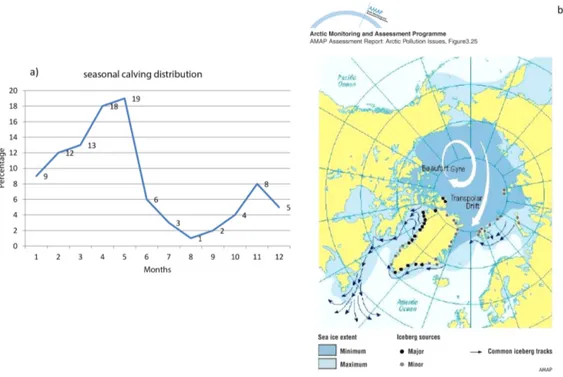
In contrast to Jongma et al. (2009, 2013), who prescribed the release position and amount of icebergs, we have cou-pled the iceberg module to GRISLI. Thus, we generate ice-bergs according to the mass loss that is calculated by GRISLI over 1 year and then given to the iceberg module. Therefore, we divide the yearly amount of mass at the calving sites into monthly values considering the seasonality of calving. We follow the results of Martin and Adcroft (2010), with the maximum occurring in spring and the minimum in late sum-mer (Fig. 2a). The monthly mass is then transformed into a daily available mass as follows in Eqs. (1) and (2):
MAM(i, j ) = TYM(i, j ) · percentage_month, (1) DAM(i, j ) = MAM(i, j )/30, (2) with MAM defining the monthly available mass at the grid point i, j ; TYM the total yearly mass at the grid point i, j ; percentage_month the percentage that is used of the TYM per month; and DAM being the daily available mass at the grid point i, j . The grid point i, j is always referring to the CLIO grid.
Furthermore, 10 size classes of bergs have been computed as defined by Bigg et al. (1997) and used and stated by e.g. Gladstone et al. (2001), Death et al. (2006) and Jongma et
Figure 2. (a) Seasonal calving distribution in percent of yearly mass per month as calculated by Martin and Adcroft (2010); (b) sites and tracks as stated in the AMAP Assessment Report (2007), reproduced with permission.
al. (2013). These size classes are based on present-day ob-servations in the Arctic done by Dowdeswell et al. (1992). Each class corresponds to a defined percentage of the daily available amount. Thus, every day we produce icebergs of the 10 different size classes as
NBS(i, j, k) = DAM(i, j ) · percentage_sizeclass(k)/ mass_sizeclass(k), (3) with NBS being the number of bergs of size class k at the grid cell i, j ; DAM the daily available mass at the grid cell i, j ; the percentage_sizeclass(k) corresponding to the percentage of DAM used for bergs of size class k; and mass_sizeclass(k) corresponding to its mass. Following Eq. (3), we get a num-ber of num-bergs per different size class at each calving site. Yet, as icebergs of the different classes can only be gener-ated if there is enough ice available, their size distribution and amount strongly depend on the ice mass as computed by GRISLI at the different locations. Using this method, the size of the calving front affects the calving mass and thus indirectly the amount of icebergs calved. But local charac-teristics, such as small glaciers producing more small bergs, are not considered since the percentage of the different size classes is the same for all calving sites. The part of the daily available mass that has not been used is saved and added to the available amount of the following day.
2.4 The coupling method and experimental set-up
We have performed four different experiments (Table 1) that vary in the implementation of the freshwater fluxes (runoff
Table 1. Summary of treatment of freshwater fluxes coming from the ice sheet and of latent heat fluxes related to iceberg melting. Runoff: basal and surface melting of the ice sheet; iceberg FWF: melt flux related to iceberg calving; direct FWF: input of calving mass as freshwater flux into the first ocean cell next to the ice-sheet margin instead of forming icebergs; local LHF: take-up of latent heat at the position where the freshwater related to iceberg melt-ing is put into the ocean; homogeneous LHF: parameterisation of freshwater fluxes related to iceberg calving as take-up of latent heat homogenously around Greenland.
Iceberg Direct Local Homogeneous Runoff FWF FWF LHF LHF
CTRL (1) – – – – X
CALV (2) X X – X –
FWFf (3) X – X – X
FWFc (4) X – X X –
and calving) calculated in GRISLI and the uptake of latent heat needed to melt the calving flux. All experiments have in common that GRISLI is coupled to iLOVECLIM apply-ing a yearly time step (Roche et al., 2014). After 1 year the monthly surface temperatures and the total amount of snow-fall are downscaled from the ECBilt to the GRISLI grid. Further, the temperature fields are vertically downscaled to overcome the large height differences between the modelled ECBilt and GRISLI surfaces. Therefore, the temperature at the highest and the lowest GRISLI point, within one ECBilt grid cell, is taken to compute a vertical lapse rate that is then
used to compute the altitude-dependent temperature at the GRISLI surface (Roche et al., 2014). The accumulation and temperature fields are needed as input fields to calculate the surface mass balance (SMB) that is defined by the accumula-tion minus ablaaccumula-tion. To obtain the ablaaccumula-tion rates, the positive degree-day (PDD) method of Fausto et al. (2009) is used, which takes into account the dependence of the ice and snow melt rate parameters on temperature as well as the depen-dence of the refreezing parameter on the altitude. After one model year, GRISLI provides the updated topography and ice mask to ECBilt to calculate the surface albedo. A more detailed description of the coupling between ECBilt, CLIO and GRISLI is given in Roche et al. (2014).
In the control (CTRL) experiment, the freshwater cycle is closed between the atmospheric model ECBilt and the oceanic model component CLIO. In ECBilt, the precipitation (solid and liquid) is computed every 4 h and the solid precip-itation is added to the snow layer. To prevent the model from piling up too much snow in areas with a positive snow mass balance, the height of the snow layer is not allowed to exceed a pre-defined threshold (10 m). If the snow layer exceeds this threshold, the amount of snow above it (the so-called excess snow) is melted, and it is added to the soil moisture (in a bucket model) and routed into the ocean when the maximum, pre-set soil water holding capacity is exceeded. In the CTRL experiment where icebergs are not explicitly modelled, their cooling effect is parameterised using the excess snow. There-fore, the heat needed to melt the excess snow is taken up ho-mogenously around Greenland from the ocean surface layer in the ocean model CLIO (Fig. 1a). The solid precipitation that is falling on the ice sheet is given to GRISLI, where it is used to calculate the surface mass balance. However, it is not removed from ECBilt because in CTRL the water cycle between ECBilt-CLIO and GRISLI is uncoupled, implying that GRISLI is not incorporated into the freshwater cycle of ECBilt–CLIO.
In the calving (CALV), the “fresh” freshwater (FWFf) and the “cold” freshwater (FWFc) experiments, the freshwater cycle is closed between ECBilt, CLIO and GRISLI. Thefore, the precipitation given from ECBilt to GRISLI is re-moved from ECBilt. GRISLI uses the precipitation to calcu-late the surface mass balance. At the end of one model year it provides ECBilt with the amount of the computed runoff (surface and basal melt) and CLIO with the ice discharge. In ECBilt the runoff is incorporated into the land routing system and distributed to the ocean. The ice discharge in CLIO is ei-ther used to generate icebergs (CALV experiment) or melted instantaneously at the ice-sheet border (FWFf and FWFc ex-periments). The ice discharge has to be melted before be-ing supplied to the ocean as a freshwater flux, and the treat-ment of the heat needed to do this differs between the CALV, FWFc and FWFf experiments. In CALV and FWFc, this heat is taken up from the ocean cell corresponding to the posi-tion where the ice discharge is added to the ocean either in the form of an iceberg melt flux (CALV) or in the form of a
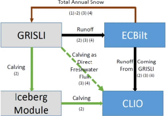
Figure 3. Schematic representation of the water cycle between the atmospheric component ECBilt, the ice-sheet module GRISLI, the iceberg module and the oceanic component CLIO; numbers corre-spond to experiments (1: CTRL; 2: CALV; 3: FWFf; 4: FWFc).
freshwater flux at the ice-sheet margin (FWFc). In FWFf the ice discharge is melted at the ice-sheet border without taking up heat; instead the latent heat related to the excess snow is taken up homogenously around Greenland, identical to the CTRL experiment. This allows us to separate the freshening and the cooling effect of icebergs.
A schematic representation of the water cycle between the atmosphere (ECBilt), ocean (CLIO), ice sheet (GRISLI) and iceberg model is displayed in Fig. 3. Volume changes of the ice sheet are reflected in the resulting calving flux and runoff. The latter is given to the land routing system of ECBilt and transported into the ocean. Runoff is included in all the ex-periments except the CTRL run.
When we compare these four experiments (Table 2), we can analyse the impact of the icebergs on the climate of the mid- to high latitudes caused by the distribution of their melt-water and the related cooling and freshening of the ocean (CALV–CTRL). Moreover, we can separately analyse the im-pact of freshening (FWFf–CTRL) and of cooling the ocean (FWFc–FWFf) as the freshwater experiments only differ in the treatment of latent heat. Further, the differences between simulated icebergs and directly applied freshwater fluxes (CALV–FWF), which ignore the spatial distribution of the meltwater, are investigated.
All runs were done under pre-industrial conditions (orbital parameters and greenhouse gas concentrations correspond-ing to the year 1850), and the ice sheet was initialised from present-day observations (Bamber et al., 2001). The exper-iments were continued until the ice sheet was equilibrated, which took about 11 000 model years. In total the experi-ments were performed for 12 000 model years, and the results of the last 1000 model years are presented in the following section. The climate is equilibrated, with no detectable drift in the deep-ocean temperature.
Table 2. Summary of anomalies analysed.
Anomaly Interpretation
CALV–CTRL Effect of non-parameterised take-up of latent heat as well as slow and spatially spread melt-ing due to movmelt-ing icebergs (i.e. coolmelt-ing, fresh-ening and distribution effect)
FWFf–CTRL Effect of freshwater (i.e. freshening)
FWFc–CTRL Effect of freshwater and non-parameterised take-up of latent heat (i.e. freshening and cool-ing effect)
FWFc–FWFf Effect of non-parameterised take-up of latent heat (i.e. cooling effect)
CALV–FWFc Effect of slower and spatially spread melting due to moving icebergs (i.e. distribution ef-fect)
CALV–FWFf Effect of non-parameterised take-up of latent heat as well as slower and spatially spread melting due to moving icebergs (i.e. cooling and distribution effect)
Figure 4. First row: ice-sheet thickness (m): (a) observed (Bam-ber et al., 2001), (b) CTRL run and (c) difference CTRL–observed; second row displays the differences (d) CALV–CTRL, (e) CALV– FWFf and (f) FWFf–CTRL (non-linear colour scheme).
3 Results
Before analysing our results, we briefly summarise the main properties of the CTRL ice sheet. In CTRL, the resulting modelled ice-sheet volume (3.8 × 10¹⁵m3)is overestimated with an excess volume of about 0.95 × 10¹⁵m3compared to observations (2.85 × 10¹⁵m3; Bamber et al., 2001). Compar-ing the CTRL volume to the computed volume usCompar-ing present-day observations as input fields to force GRISLI displays that dynamically coupling GRISLI to ECBilt results in an excess ice-sheet volume of 4.4 × 10¹⁴m3(Roche et al., 2014). The ice sheet (Fig. 4b) extends almost everywhere down to the Greenland coast, even in regions that are currently ice-free
Figure 5. 1000-year averages. First row: mass balance (m): (a) CTRL, (b) CALV and (c) FWFf; 2nd row: accumulation (m): (d) CTRL, (e) CALV and (f) FWFf (non-linear colour scheme).
according to observations (Fig. 4a). Further, the CTRL ice sheet is too thin (by up to 500 m) in northwest Greenland but too thick in central and northeast Greenland (by up to 1000 m) and over Devon Island. This can be explained by the overestimation of the positive SMB by GRISLI compared to the SMB modelled by a regional climate model MAR (not shown; Fettweis et al., 2013). The computed SMB (Fig. 5a) captures the overall pattern of positive SMB in the south and less in the north of Greenland, and negative SMB along the coast. Yet, GRISLI overestimates the positive SMB resulting in the excessive extension and ice-sheet thickness. The com-puted SMB (Fig. 5a) captures the overall pattern of positive SMB in the south and less in the north of Greenland, and negative SMB along the coast. Yet, GRISLI overestimates the positive SMB resulting in the excessive extension and ice-sheet thickness. This is also seen in the computed sur-face mass balance of the CTRL ice sheet (648 Gt yr−1, Ta-ble 3), which is about one-third higher than computed with a regional climate model (469 Gt yr−1; Ettema et al., 2009) in accordance with the overestimated volume.
3.1 Representation of icebergs compared to observations
The results of the CALV experiment reveal that the modelled calving sites and iceberg tracks fit the observations reason-ably well. As is shown in the Arctic Monitoring and As-sessment Programme (AMAP) plot (Fig. 2b), calving oc-curs along almost the entire coast of Greenland, with major calving sites in Baffin Bay and along the southeast coast of Greenland. Despite the coarse resolution of GRISLI and the simplified calving scheme used, these calving sites are gen-erally well captured (Fig. 6a). The sites in the northeast of Greenland are overestimated, which is probably caused by overestimated ice-sheet thickness there compared to obser-vations (Fig. 4b compared to a). The modelled calving flux (2.0 × 10⁻²Sv, Table 3) is almost twice as large as indicated
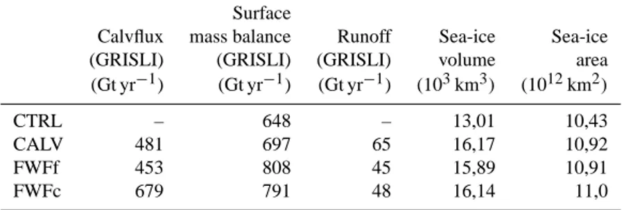
Table 3. Summary of computed ice discharge (Calvflux) as calculated in GRISLI, surface mass balance (SMB) of the Greenland ice sheet, runoff as calculated in GRISLI, and sea-ice volume and area as computed in CLIO.
Surface
Calvflux mass balance Runoff Sea-ice Sea-ice (GRISLI) (GRISLI) (GRISLI) volume area (Gt yr−1) (Gt yr−1) (Gt yr−1) (103km3) (1012km2)
CTRL – 648 – 13,01 10,43
CALV 481 697 65 16,17 10,92
FWFf 453 808 45 15,89 10,91
FWFc 679 791 48 16,14 11,0
Figure 6. (a) Number of icebergs being generated per year; (b) number of icebergs moving within a grid cell per year. Icebergs moving within one grid cell for a longer period are counted more than once (non-linear colour scheme).
by present-day observations that range from 0.8 × 10⁻²Sv (Church et al., 2001) to 1.0 × 10⁻²Sv (Hooke, 2005), which is due to the simplified calving method that assumes calving as soon as the ice sheet’s thickness is below 150 m, and partly due to the applied pre-industrial forcing, producing a colder climate than observed today (Kobashi et al., 2011).
The mean yearly distribution of icebergs (Fig. 6b) illus-trates that the majority of bergs travels along the east and west coast of Greenland reaching as far south as about 50◦N with a few bergs moving further south and even travelling up to Europe. The transportation of the icebergs depends on both the winds and ocean currents. But it can be seen that most bergs calved east of Greenland are transported southward due to the northerly winds and the East Greenland Current and the ones calved west of the GrIS are first moved northward by the West Greenland Current and then southward again by the Baffin Island and Labrador Currents (Fig. 6b). Further, the icebergs calved along the north coast of the GrIS are dis-tributed in the Arctic Ocean by the Beaufort Gyre and the prevailing winds. These modelled patterns fit well with ob-servations (Fig. 2b) and are also found in the model study of Bigg et al. (1996).
3.2 Impact of icebergs on the pre-industrial climate and the Greenland ice sheet
(cooling–freshening–distribution effect)
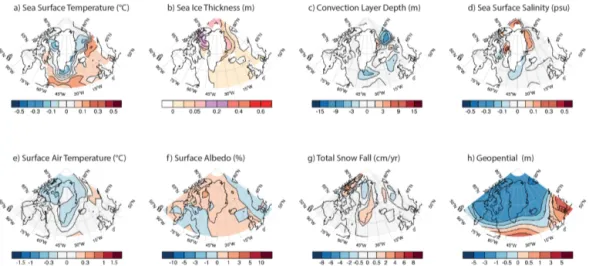
We find that including icebergs in the model set-up (CALV experiment) causes a cooler ocean state than the CTRL run around Greenland (Fig. 7a). This is due to the transporta-tion of the icebergs by winds and ocean currents, leading to a more extensive distribution of the meltwater, reaching up to Svalbard and Iceland (Fig. 1d). In accordance with the ice-bergs’ melt flux, the sea surface temperatures (SSTs, Fig. 7a) decrease around the GrIS as a result of the take-up of la-tent heat needed to melt the icebergs as well as the incom-ing cold meltwater (Fig. 1b, d). Strong differences are found in Baffin Bay due to the large number of icebergs in this region. The increased melt flux enhances the sea-ice thick-ness (SIT) up to 0.7 m (Fig. 7b). In Baffin Bay the response in sea surface salinity (SSS, Fig. 7d) is two-sided. North of 65◦N there are lower values due to the icebergs’ freshening
effect, but south of 65◦N we find higher SSS in CALV than
in CTRL due to enhanced brine rejection by the thickened sea ice (Fig. 7b). In Hudson Bay the lower SSTs due to the parameterisation used in CTRL (Fig. 1a) causes less evapora-tion and thus lower SSS than in CALV (Fig. 7d). Also in the Labrador Sea including icebergs causes a decrease of SST by up to −0.5◦C (Fig. 7a) because their meltwater enhances the ocean’s stratification, thereby weakening the deep convection and the mixing of the upper water columns with the underly-ing warmer and saltier waters (Fig. 7c, d). In the Greenland, Iceland and Norwegian (GIN) seas, however, the icebergs freshen the ocean surface and cause a shift of the centre of the deep convection site southward without a change in the convective activity (Fig. 7c). The shifted centre is also seen in the SST and SSS patterns, with locally higher values being found north of Iceland in CALV than in CTRL.
A thicker sea-ice cover in combination with a higher albedo and generally lower SSTs cause a cooler atmospheric state (Fig. 7e, f) in CALV compared to CTRL, since less heat is exchanged between the ocean and the atmosphere. Thus, the air temperatures over the whole region decrease by up to
−2◦C (Fig. 7e). This changed temperature field is linked to an altered atmospheric circulation pattern with high-pressure
Figure 7. CALV–CTRL differences of 1000-year averages: (a) sea surface temperature, SST (◦C, non-linear colour scheme); (b) sea-ice thickness (m, non-linear colour scheme); (c) convection layer depth, CLD (m); (d) sea surface salinity, SSS (psu); (e) air temperature, TAIR (◦C); (f) surface albedo, ALB (%, non-linear colour scheme); (g) total snowfall, SNOW (cm yr−1, non-linear colour scheme); (h) geopotential (m, non-linear colour scheme).
anomalies over central Greenland (Fig. 7h). This is linked to less snowfall at the centre of the ice sheet and more along the ice-sheet border (Fig. 7g), which is also partly seen in the re-sulting accumulation patterns of CALV and CTRL (Fig. 5d, e). In southeastern Greenland the altered snowfall pattern re-sults in a thinner ice sheet than in CALV (Fig. 4c, 7g). More-over, the colder surface temperatures over the ice sheet and especially western Greenland decrease the ablation zone in CALV (Fig. 6a, b). This causes an increase in thickness of the western ice sheet’s margin by up to 300 m in CALV. This fits better to the observed GrIS height than the CTRL exper-iment, where we find an underestimation of the ice sheet’s thickness in western and an overestimation in eastern Green-land compared to observations (Fig.4c).
From the comparison of CALV with CTRL we conclude that icebergs cause an overall colder climate in the mid- to high latitudes. This pattern is not captured by the homoge-neous uptake of latent heat in the CTRL run because the pa-rameterisation of icebergs used underestimates the freshen-ing and coolfreshen-ing (Fig. 1a, b). Overall, the CALV ice sheet is too extensive and thick compared to observations, as is the CTRL one. But explicitly modelling icebergs increases (de-creases) the ice-sheet thickness along the western (eastern) Greenland margin (Fig. 4c), which fits better to observations (not shown). This is caused by the local effect of the icebergs on the sea-ice thickness and the atmospheric temperatures.
3.3 Parameterising icebergs using freshwater fluxes – how well does it work?
3.3.1 The freshening effect (FWFf–CTRL)
In the FWFf experiment the calving flux (1.9 × 10⁻²Sv, Table 3) is released instantaneously at the calving sites
(Fig. 1e), consequently introducing meltwater at 0◦C to the upper ocean layer that freshens and cools it and causes a cooler mid- to high-latitude climate compared to CTRL. But the heat needed to melt the ice discharge is not taken up from the ocean; instead the FWFf and CTRL set-up share the same parameterisation of homogeneous take-up of la-tent heat (Fig. 1a). The FWFf experiment results in up to 0.5◦C colder SST (Fig. 8a) than CTRL, particularly around the GrIS, with the strongest differences in the calving re-gions, such as Baffin Bay, or in regions of deep-ocean con-vection. We find increased sea-ice thickness in FWFf because of the colder ocean state, especially north of 65◦N where it grows up to 0.6 m thicker compared to CTRL (Fig. 8b). The deep-ocean convection site in the Labrador Sea is close to the GrIS margin and thus especially sensitive to the ice sheet’s ice discharge that weakens the convection and stabilises the water column, as can be seen in the colder and fresher sur-face ocean layer (Fig. 8a, c, d). The opposite is seen in the GIN seas, where the ocean convection is enhanced and the centre shifted westwards in FWFf. The colder SSTs close to the Greenland margin promote deep mixing, which causes higher SST and higher SSS values north of Iceland. Due to the shift of convection centre, there is less upwelling of warm and salty water in the Norwegian Sea, as can be directly seen in the SST and SSS (Fig. 8a, d).
The altered ocean conditions in FWFf compared to CTRL are evident in the increased surface albedo due to the thick-ened sea ice. Its shielding effect causes lower air tempera-tures of up to −1.5◦C (Fig. 8b, e). In FWFf there is less snowfall in the centre of Greenland up to the Denmark Strait and more along the margins than in CTRL (Fig. 8g). Due to the colder conditions in Baffin Bay, the ablation zone is smaller in FWFf than in CTRL (Fig. 5c). This is also
re-Figure 8. FWFf–CTRL differences of 1000-year averages: (a) sea surface temperature, SST (◦C, non-linear colour scheme); (b) sea-ice thickness (m, non-linear colour scheme); (c) convection layer depth, CLD (m); (d) sea surface salinity, SSS (psu); (e) air temperature, TAIR (◦C); (f) surface albedo, ALB (%, non-linear colour scheme); (g) total snowfall, SNOW (cm yr−1, non-linear colour scheme); (h) geopotential (m, non-linear colour scheme).
flected in the ice-sheet height of FWFf along the western margin (Fig. 5e). This is in contrast to the thinner eastern margin (up to 500 m) than CTRL that results from less ac-cumulation and an enhanced negative surface mass balance (Fig. 6c, f).
3.3.2 The distribution effect (CALV–FWFc)
Applying the calving fluxes in the form of instantaneous freshwater fluxes (2.0 × 10⁻²Sv, Table 3) that do take-up the latent heat needed to melt them at the calving sites (FWFc) both freshens and cools the ocean close to the GrIS margin (Fig. 1c, e). At the end of the FWFc experiment, the simu-lated climate and ice-sheet configuration are similar to CALV (not shown). Even though the take-up of latent heat, due to the melt of icebergs, is spatially more restricted in FWFc than in CALV (Fig. 1b, c), the effect on the ocean (Table 3), the atmosphere and the GrIS is comparable to CALV (not shown). Therefore, the spatial pattern of the uptake of latent heat and released freshwater (distribution effect, Fig. 1) re-lated to the movement of the icebergs is relatively small un-der pre-industrial conditions.
3.3.3 The cooling and distribution effect (CALV–FWFf)
Using the calving mass calculated by GRISLI to generate icebergs (as in CALV) that freshen and cool the ocean un-evenly instead of applying this mass in the form of local freshwater fluxes and homogenous take-up of latent heat (as in FWFf) results in different ice-sheet topographies at the end of the experiments. Explicitly modelling icebergs has a stronger cooling effect close to the Greenland ice sheet than FWFf, since most of the iceberg melt flux (IMF) is released
close to the ice sheet. The melting of icebergs extracts heat from the upper layers of the ocean, depending on the size and the number of bergs (Fig. 1b, d). In FWFf, however, this spatial pattern of take-up of latent heat is ignored. Therefore, CALV results in lower SST values (−0.2◦C) around the GrIS and in higher values (+0.2◦C) further away. Moreover, the stronger cooling in CALV allows for a thicker SIT than in FWFf (Fig. 9b), especially in Baffin Bay where a lot of ice-bergs are generated as well as transported to.
In the Labrador and GIN seas the explicit modelling of ice-bergs causes a weakened convection compared to FWFf be-cause the icebergs withdraw the latent heat they need to melt from the respective ocean layer, thereby stabilising the wa-ter column. Due to the distribution of icebergs, less melt flux is released in the Greenland Sea than in FWFf because the calved bergs are moved southward (Fig. 1f). This is displayed in the higher SSS (0.2 psu) compared to FWFf (Fig. 9d).
The small differences in the resulting ocean state are also reflected in the atmosphere, which displays lower temper-atures (−0.5◦C) over Greenland and North America but higher temperatures over the North Atlantic and Iceland and Norwegian seas (Fig. 9e) as well as a slightly changed snow-fall pattern (Fig. 9g). Nevertheless, these relatively small dif-ferences cause thinner ice-sheet thicknesses up to 150 m in southern Greenland because in FWFf there is less accumula-tion and the warmer surface temperatures cause more abla-tion than in CALV (Fig. 5b, c, e, f).
From our studies we conclude that the experiments with the freshwater fluxes from the ice sheet (runoff and calv-ing) implemented (CALV, FWFf, FWFc) result in a colder climate than CTRL and an up to 300 m altered ice-sheet thickness. Even though the resulting ocean and atmospheric state is comparable in all the freshwater experiments, the sheet topographies vary up to 150 m. The differences in
ice-Figure 9. CALV–FWFf differences of 1000-year averages: (a) sea surface temperature, SST (◦C, non-linear colour scheme); (b) sea-ice thickness (m, non-linear colour scheme); (c) convection layer depth (CLD) (m); (d) sea surface salinity, SSS (psu); (e) air temperature, TAIR (◦C); (f) surface albedo, ALB (%, non-linear colour scheme); (g) total snowfall, SNOW (cm yr−1, non-linear colour scheme); (h) geopotential (m, non-linear colour scheme).
sheet thickness arise due to the different spatial pattern of the added calving flux, either directly at the calving site (FWFf, FWFc) or distributed by the icebergs (CALV), and especially due to the spatial pattern of the take-up of latent heat needed to melt it. Using local freshwater and latent heat fluxes to parameterise icebergs (FWFc) results in a similar ice sheet and climate as the explicit modelling of icebergs (CALV), whereas the differences are stronger if the take-up of latent heat is computed homogenously (FWFf).
4 Discussion
In the presented study the coupling between the ice-sheet model GRISLI and the earth system model of intermediate complexity iLOVECLIM and the dynamical iceberg module was further developed. This set-up was used to investigate the impact of icebergs on climate and the ice sheet itself in a fully coupled low-resolution model. Modelling iceberg calv-ing is a complex task as small-scale processes are involved which we cannot expect to represent with the 40 × 40 km resolution of GRISLI. Still, the calculated calving sites fit reasonably to observations, as do the modelled iceberg tra-jectories. Moreover, as we are particularly interested in the mechanisms behind the impact of icebergs on both the cli-mate and the ice sheet, we would argue that these are rel-atively insensitive to the ice-sheet model resolution. Never-theless, the modelled calving sites and iceberg trajectories fit reasonably to the observations. This is the calving flux is twice as large as currently observed, due to the ice sheet’s model resolution, which might result in an overestimated im-pact of the icebergs. Another potential limitation is that the refreezing of the meltwater, as well as splitting-up of bergs, is not accounted for. Excluding this latter process probably
leads to an underestimation of the spread of the freshwater anomaly, but an overestimation of the near-shore freshwater input, as has been reported by Martin and Adcroft (2010). This could explain the less extensive spread of the iceberg melt flux in our simulations compared to theirs. Despite the aforementioned shortcomings, this model set-up is a valuable tool with which to investigate the effect of icebergs on the climate of the mid- to high latitudes and the Greenland ice sheet, especially as the EMIC is coupled to a dynamically computed ice-sheet model and therefore changes in calving rates and positions are taken into account. This is of particu-lar interest for the study of past climate changes at relatively long timescales (centennial to multi-millennia), when large changes in the ice-sheet geometry can also be expected.
So far, icebergs have mostly been parameterised using freshwater fluxes to save computation time. To study the im-pact of such parameterisations, we compared dynamically included icebergs to freshwater fluxes released at the same locations and according to the same seasonal cycle as the icebergs and found noticeable differences. Icebergs cause thicker sea ice all around Greenland and especially in Baf-fin Bay and the Arctic Ocean compared to the freshwater fluxes being applied at the calving locations together with homogeneous take-up of latent heat around Greenland. This is comparable to the findings of Jongma et al. (2009), who performed sensitivity studies under pre-industrial conditions, where they investigated the different impact of icebergs com-pared to homogeneously distributed freshwater fluxes south of 55◦ in the Southern Ocean. They found that the effect of icebergs is restricted closer to shore than the freshwater fluxes and that the sea-ice formation is facilitated by ice-bergs. Yet, when we apply local freshwater fluxes that cool the ocean locally due to the take-up of latent heat, these dif-ferences decrease, and in regions where more freshwater is
released directly than in the form of icebergs these fluxes are generally more efficient in producing thicker sea ice. This is in agreement with Martin and Adcroft (2010), who in-vestigated the impact of interactively coupled icebergs in an atmosphere–ocean GCM and also compared it to directly ap-plied freshwater fluxes. They find a decrease in sea-ice thick-ness almost everywhere around Antarctica besides a few re-gions when generating icebergs. Hunke and Comeau (2011) also investigated the interactions between sea ice and both giant and small icebergs in the Southern Ocean using a stand-alone ocean model with explicitly included icebergs that are moved according to the ocean currents and the atmospheric forcing applied. They revealed that the bergs locally affect the sea-ice thickness and area but conclude that on a global scale these dynamically induced differences are negligible. In our study the effects on sea ice are over a bigger spatial scale and have an extensive impact via feedback mechanisms on the atmosphere and consequently the development of the ice sheet. In most regions, the experiment with the explicitly modelled icebergs enhances the sea-ice thickness stronger than the other freshwater experiments because of both the freshening and the cooling effect as the bergs take up the la-tent heat from the ocean. These findings coincide with the results of Jongma et al. (2013), who investigated the impact of icebergs on climate during Heinrich events. They show that including icebergs as meltwater fluxes and take-up of la-tent heat has a stronger impact on climate than just meltwater fluxes.
The presented coupled model set-up offers a great ap-proach to conduct long-term experiments to better under-stand the role of icebergs and the interactions between the different climate components during abrupt climate changes. This is feasible with the presented model since the compu-tation time for 1000 model years is about 2 days in the fully coupled set-up. A useful next step could be to use this model set-up to study Heinrich events in detail, as the crucial ques-tion as to how the icebergs’ feedback was on climate under colder and more instable times has not yet been fully ad-dressed.
5 Conclusions
We have coupled the ice-sheet model GRISLI to the earth system model iLOVECLIM to study the impact of dynamical-thermodynamical icebergs on climate and the Greenland ice sheet under pre-industrial conditions. We find that the modelled calving sites correspond well with present-day observations with a slight underestimation of the calving along the southeastern margin of Greenland. The amount of ice being calved is almost 2 times the value observed for the present-day climate, which can be explained by the colder pre-industrial than present-day climate conditions and the simple calving method used. Further, the main iceberg routes are reproduced using the modelled winds and ocean currents.
According to our study, implementing the freshwater fluxes (calving and runoff) from the Greenland ice sheet causes a colder climate at mid- to high latitudes. Explic-itly including icebergs results in an increased sea-ice thick-ness all around the Greenland ice sheet, especially north of 65◦N. Consequently, we find higher surface albedo values and a weakened sensible heat flux, due to its shielding ef-fect. Therefore, icebergs cause cooler air temperatures above Greenland and a shift in the atmospheric pattern, which is linked to decreased snowfall over central and southern Greenland and an increased one at the ice-sheet border. The colder prevailing temperatures and the changed accumula-tion pattern lead to a thicker western ice-sheet height and a thinner eastern ice sheet (up to 300 m), which fit better to observations.
From the presented analysis we conclude that the strongest impact of calving on the climate is due to the spatial distri-bution of the take-up of latent heat needed to melt the ice mass and that the freshening due to the released meltwater has a smaller impact. Applying direct freshwater fluxes that absorb the latent heat locally at the calving sites results in a similar climate and ice-sheet geometry as in the CALV exper-iment. However, directly applied freshwater fluxes together with homogenous take-up of latent heat lead to an underes-timated cooling at the ice-sheet border and an overesunderes-timated one temperatures further away. The warmer surface tempera-tures over southern Greenland cause higher ablation rates and result in a 150 m reduction in ice-sheet thickness compared to the iceberg experiment.
In the present study the resulting climate conditions and ice-sheet geometries differ between the experiments even though they were done under pre-industrial conditions where the calving rates are relatively constant and small. The im-pact of icebergs on the ice sheet’s development is thought to be stronger during colder climate conditions with higher calving rates.
Acknowledgements. M. Bügelmayer is supported by NWO through the VIDI/AC2ME project no. 864.09.013. D. M. Roche is supported by NWO through the VIDI/AC2ME project no. 864.09.013 and by CNRS-INSU. The authors wish to thank Christophe Dumas for his advice and help in the coupling of the ice-sheet model to the iceberg module and Catherine Ritz for the use of the GRISLI ice-sheet model. Further, the authors wish to thank the reviewers for provid-ing constructive comments on how to improve the quality of this paper. The authors also gratefully acknowledge the Institute Pierre Simon Laplace for hosting the iLOVECLIM model code under the LUDUS framework project (https://forge.ipsl.jussieu.fr/ludus). This is NWO/AC2ME contribution number 06.
References
Arctic Monitoring and Assessment Programme (AMAP), AMAP Assessment Report: Arctic Pollution Issues, Figure 3–25, 2007 Bamber, J. L., Layberry, R. L., and Gogineni, S.: A new ice
thick-ness and bed data set for the Greenland ice sheet 1. Measurement, data reduction, and errors, J. Geophys. Res., 106, 33773–33780, doi:10.1029/2001JD900054, 2001.
Bigg, G. R., Wadley, M. R., Stevens, D. P., and Johnson, J. V.: Pre-diction of iceberg trajectories for the North Atlantic and Arctic Oceans, Geophys. Res. Lett., 23, 3587–3590, 1996.
Bigg, G. R., Wadley, M. R., Stevens, D. P., and Johnson, J. V.: Mod-elling the dynamics and thermodynamics of icebergs, Cold Reg. Sci. Technol., 26, 113–135, doi:10.1016/S0165-232X(97)00012-8, 1997.
Bonelli, S., Charbit, S., Kageyama, M., Woillez, M.-N., Ramstein, G., Dumas, C., and Quiquet, A.: Investigating the evolution of major Northern Hemisphere ice sheets during the last glacial-interglacial cycle, Clim. Past, 5, 329–345, doi:10.5194/cp-5-329-2009, 2009.
Box, J. E.: Greenland ice sheet mass balance reconstruction. Part II: surface mass balance (1840–2010), J. Climate, 26, 6974–6989, doi:10.1175/JCLI-D-12-00518.1, 2013.
Broccoli, A. J.: Tropical cooling at the Last Glacial Maximum: an atmosphere- mixed layer ocean model simulation, J. Climate, 13, 951–976, 2000.
Brovkin, V., Ganopolski, A., and Svirezhev, Y.: A continuous climate-vegetation classification for use in climate-biosphere studies, Ecol. Modell., 101, 251–261, 1997.
Campin, J. M. and Goosse, H.: A parameterization of density driven downsloping flow for coarse resolution model in z-coordinate, Tellus, 51A, 412–430, 1999.
Charbit, S., Ritz, C., Philippon, G., Peyaud, V., and Kageyama, M.: Numerical reconstructions of the Northern Hemisphere ice sheets through the last glacial-interglacial cycle, Clim. Past, 3, 15–37, doi:10.5194/cp-3-15-2007, 2007.
Church, J. A., Gregory, J. M., Huybrechts, P., Kuhn, M., Lambeck, K., Nhuan, M. T., Qin, D., and Woodworth, P. L.: Changes in sea level, in: Climate Change 2001: The Scientific Basis: Con-tribution of Working Group I to the Third Assessment Report of the Intergovernmental Panel on Climate Change, edited by: Houghton, J. T., Ding, Y., Griggs, D. J., Noguer, M., Van der Lin-den, P. J., Dai, X., Maskell, K., and Johnson, C. A., Cambridge University Press, Cambridge, 639–694, 2001.
Clark, P. U.: Northern Hemisphere Ice sheet Influences on Global Climate Change, Science, 286, 1104–1111, doi:10.1126/science.286.5442.1104, 1999.
Claussen, M., Weaver, A., Crucifix, M., Fichefet, T., Loutre, M.-F., Weber, S. L., Alcamo, J., Alexeev, V. A., Berger, A., Calov, R., Ganopolski, A., Goosse, H., Lohmann, G., Lunkeit, F., Mokhov, I. I., Petoukhov, V., Stone, P., and Wang, Z.: Earth system mod-els of intermediate complexity: closing the gap in the spec-trum of climate system models, Clim. Dynam., 18, 579–586, doi:10.1007/s00382-001-0200-1, 2002.
Death, R., Siegert, M. J., Bigg, G. R., and Wadley, M. R.: Mod-elling iceberg trajectories, sedimentation rates and meltwater in-put to the ocean from the Eurasian Ice Sheet at the Last Glacial Maximum, Palaeogeogr., Palaeoclim., Palaeoecol., 236, 135– 150, doi:10.1016/j.palaeo.2005.11.040, 2006.
Deleersnijder, E. and Campin, J.-M.: On the computation of the barotropic mode of a free-surface world ocean model, Ann. Geo-phys., 13, 675–688, 1995,
http://www.ann-geophys.net/13/675/1995/.
Deleersnijder, E., Beckers, J.-M., Campin, J.-M., El Mohajir, M., Fichefet, T., and Luyten, P.: Some mathematical problems asso-ciated with the development and use of marine models, in: The mathematics of model for climatology and environment, edited by: Diaz, J. I., NATO ASI Series, Vol. I 48, Springer-Verlag, 39– 86, 1997.
Dowdeswell, J. A., Whittington, R. J., and Hodgkins, R.: The Sizes, Frequencies, and Freeboards of East Greenland Icebergs Ob-served Using Ship Radar and Sextant, J. Geophys. Res., 97, 3515–3528, 1992.
Ettema, J., Van Den Broeke, M. R., Van Meijgaard, E., Van De Berg, W. J., Bamber, J. L., Box, J. E., and Bales, R. C.: Higher surface mass balance of the Greenland ice sheet revealed by high-resolution climate modeling, Geophys. Res. Lett., 36, 4–8, doi:10.1029/2009GL038110, 2009.
Fausto, R. S., Ahlström, A. P., As, D. V. A. N., Bøggild, C., E. and Johnsen, S. J.: A new present-day tempera-ture parameterization for Greenland, J. Glaciol., 55, 95–105, doi:10.3189/002214309788608985, 2009.
Fettweis, X., Franco, B., Tedesco, M., van Angelen, J. H., Lenaerts, J. T. M., van den Broeke, M. R., and Gallée, H.: Estimating the Greenland ice sheet surface mass balance contribution to fu-ture sea level rise using the regional atmospheric climate model MAR, The Cryosphere, 7, 469–489, doi:10.5194/tc-7-469-2013, 2013.
Fichefet, T. and Morales Maqueda, M. A.: Sensitivity of a Global sea ice model to the treatment of ice thermodynamics and dy-namics, J. Geophys. Res., 102, 12609–12646, 1997.
Fichefet, T. and Morales Maqueda, M. A.: Modelling the influence of snow accumulation and snow-ice formation on the seasonal cycle of the Antarctic sea-ice cover, Clim. Dynam., 15, 251–268, 1999.
Gates, W. L.: Modeling the ice-age climate, Science, 191, 1138– 1144, 1976.
Gladstone, R. M., Bigg, G. R., and Nicholls, K. W.: Iceberg trajec-tory modeling and meltwater injection in the Southern Ocean, J. Geophys. Res., 106, 19903–19915, doi:10.1029/2000JC000347, 2001.
Goelzer, H., Huybrechts, P., Loutre, M. F., Goosse, H., Fichefet, T., and Mouchet, A.: Impact of Greenland and Antarctic ice sheet in-teractions on climate sensitivity, Clim. Dynam., 37, 1005–1018, doi:10.1007/s00382-010-0885-0, 2010.
Goosse, H., Brovkin, V., Fichefet, T., Haarsma, R., Huybrechts, P., Jongma, J., Mouchet, A., Selten, F., Barriat, P.-Y., Campin, J.-M., Deleersnijder, E., Driesschaert, E., Goelzer, H., Janssens, I., Loutre, M.-F., Morales Maqueda, M. A., Opsteegh, T., Mathieu, P.-P., Munhoven, G., Pettersson, E. J., Renssen, H., Roche, D. M., Schaeffer, M., Tartinville, B., Timmermann, A., and Weber, S. L.: Description of the Earth system model of intermediate complex-ity LOVECLIM version 1.2, Geosci. Model Dev., 3, 603–633, doi:10.5194/gmd-3-603-2010, 2010.
Green, C. L., Green, J. A. M., and Bigg, G. R.: Simulating the im-pact of freshwater inputs and deep-draft icebergs formed during a MIS 6 Barents Ice Sheet collapse, Paleoceanography, 26, 1–16, doi:10.1029/2010PA002088, 2011.
Gregory, J. M., Browne, O. J. H., Payne, A. J., Ridley, J. K., and Rutt, I. C.: Modelling large-scale ice-sheet-climate inter-actions following glacial inception, Clim. Past, 8, 1565–1580, doi:10.5194/cp-8-1565-2012, 2012.
Greve, R.: Thermomechanisches Verhalten polythermer Eiss-childe – Theorie, Analytik, Numerik, PhD thesis, Institut fuer Mechanik, Technische Hochschule Darmstadt, Germany, 1995. Greve, R.: Application of a polythermal three-dimensional ice sheet
model to the Greenland ice sheet: response to steady-state and transient climate scenarios, J. Climate, 10, 901–918, 1997. Hanna, E., Huybrechts, P., Cappelen, J., Steffen, K., Bales, R.
C., Burgess, E., McConnell, J. R., Peder Steffensen, J., Van den Broeke, M., Wake, L., Bigg, G. R., Griffiths, M., and Savas, D.: Greenland Ice Sheet surface mass balance 1870 to 2010 based on Twentieth Century Reanalysis, and links with Global climate forcing, J. Geophys. Res., 116, D24121, doi:10.1029/2011JD016387, 2011.
Helm, V., Humbert, A., and Miller, H.: Elevation and elevation change of Greenland and Antarctica derived from CryoSat-2, The Cryosphere, 8, 1539–1559, doi:10.5194/tc-8-1539-2014, 2014.
Hemming, S. R.: Heinrich events: Massive late Pleistocene detritus layers of the North Atlantic and their global climate imprint, Rev. Geophys., 42, RG1005, doi:10.1029/2003RG000128, 2004. Hooke, R. L.: Principles of Glacier Mechanics, 2nd Ed., Cambridge
University Press, Cambridge, 2005.
Hunke, E. C. and Comeau, D.: Sea ice and iceberg dynamic inter-action, J. Geophys. Res., 116, 1–9, doi:10.1029/2010JC006588, 2011.
Hutter, K.: Theoretical Glaciology: Material Science of Ice and the Mechanics of Glaciers and Ice Sheets, D. Reidel, 510 pp., 1983. Huybrechts, P.: A 3-D model for the Antarctic ice sheet: a sensitivity study on the glacial-interglacial contrast, Clim. Dynam., 5, 79– 92, 1990.
Huybrechts, P. and de Wolde, J.: The dynamic response of the Greenland and Antarctic ice sheets multiple-century climatic warming, J. Climate, 12, 2169–2188, 1999.
Huybrechts, P., Gregory, J., Janssens, I., and Wild, M.: Modelling Antarctic and Greenland volume changes during the 20th and 21st centuries forced by GCM time slice integrations, Global Planet. Change, 42, 83–105, 2004.
Jongma, J. I., Driesschaert, E., Fichefet, T., Goosse, H., and Renssen, H.: The effect of dynamic–thermodynamic icebergs on the Southern Ocean climate in a three-dimensional model, Ocean Modell., 26, 104–113, doi:10.1016/j.ocemod.2008.09.007, 2009. Jongma, J. I., Renssen, H., and Roche, D. M.: Simulating Heinrich event 1 with interactive icebergs, Clim. Dynam., 40, 1373–1385, doi:10.1007/s00382-012-1421-1, 2013.
Kageyama, M., Charbit, S., Ritz, C., and Khodri, M.: Quantifying ice-sheet feedbacks during the last glacial inception, Geophys. Res. Lett., 31, L24203, doi:10.1029/2004GL021339, 2004. Kobashi, T., Kawamura, K., Severinghaus, J. P., Barnola, J.-M.,
Nakaegawa, T., Vinther, B. M., Johnsen, S. J., and Box, J. E.: High variability of Greenland surface temperature over the past 4000 years estimated from trapped air in an ice core, Geophys. Res. Lett., 38, L21501, doi:10.1029/2011GL049444, 2011. Levine, R. C. and Bigg, G. R.: Sensitivity of the glacial ocean to
Heinrich events from different iceberg sources, as modeled by
a coupled atmosphere-iceberg-ocean model, Paleoceanography, 23, PA4213, doi:10.1029/2008PA001613, 2008.
Loset, S.: Thermal-Energy Conservation in Icebergs and Track-ing by Temperature, J. Geophys. Res.-Oceans, 98, 10001–10012, 1993.
MacAyeal, D. R.: Large Scale ice flow over a vicous basal Sedi-ment: Theory and Application to Ice Stream B, Antarctica, Geo-phys. Res., 94, 4071–4087, 1989.
Martin, T. and Adcroft, A.: Parameterizing the fresh-water flux from land ice to ocean with interactive icebergs in a coupled climate model, Ocean Modell., 34, 111–124, doi:10.1016/j.ocemod.2010.05.001, 2010.
Morland, L.: Thermo-mechanical balances of ice sheet flow, Geo-phys. AstroGeo-phys. Fluid Dynam., 29, 237–266, 1984.
Mueller, D. R., Vincent, W. F., and Jeffries, M. O.: Break-up of the largest Arctic ice shelf and associated loss of an epishelf lake, Geophys. Res. Lett. 30, 2031, doi:10.1029/2003GL017931, 2003.
Nick, F. M., Vieli, A., Howat, I. M., and Joughin, I.: Large-scale changes in Greenland outlet Glacier dynamics triggered at the terminus, Nat. Geosci., 2, 110–114, doi:10.1038/ngeo394, 2009. Opsteegh, J. D., Haarsma, R. J., Selten, F. M., and Kattenberg, A.: ECBilt: A dynamic alternative to mixed boundary conditions in ocean models, Tellus, 50A, 348–367, 1998.
Peyaud, V., Ritz, C., and Krinner, G.: Modelling the Early We-ichselian Eurasian Ice Sheets: role of ice shelves and influence of ice-dammed lakes, Clim. Past, 3, 375–386, doi:10.5194/cp-3-375-2007, 2007.
Pollard, D.: A retrospective look at coupled ice sheet–climate mod-eling, Clim. Change, 100, 173–194, doi:10.1007/s10584-010-9830-9, 2010.
Pollard, D. and DeConto, R. M.: A coupled sheet/ ice-shelf/sediment model applied to a marine margin flow- line: forced and unforced variations, in: Glacial sedimentary pro-cesses and products, edited by: Hambrey, M. J., Christoffersen, P., Glasser, N. F., and Hubbard, B. Malden, MA, Blackwell, 37– 52, 2007.
Pollard, D. and Thompson, S. L.: Climate and ice-sheet mass bal-ance at the Last Glacial Maximum from the GENESIS version 2 global climate model, Quaternary Sci. Rev., 16, 841–864, 1997. Ridley, J. K.: Elimination of the Greenland Ice Sheet in a High CO2
Climate, J. Climate, 18, 3409–3427, 2005.
Rignot, E. and Kanagaratnam, P.: Changes in the velocity struc-ture of the Greenland Ice Sheet, Science, 311, 986–990, doi:10.1126/science.1121381, 2006.
Rignot, E., Mouginot, J., and Scheuchl, B.: Ice flow of the Antarctic ice sheet, Science, 333, 1427–1430, doi:10.1126/science, 2011. Ritz, C., Fabre, A., and Letréguilly, A.: Sensitivity of a
Green-land ice sheet model to ice flow and ablation parameters: con-sequences for the evolution through the last climatic cycle, Clim. Dynam., 13, 11–23, doi:10.1007/s003820050149, 1997. Ritz, C., Rommelaere, V., and Dumas, C.: Modeling the evolution
of Antarctic ice sheet over the last 420,000 years: Implications for altitude changes in the Vostok region, J. Geophys. Res., 106, 31943–31964, doi:10.1029/2001JD900232, 2001.
Roche, D. M., Wiersma, A. P., and Renssen, H.: A systematic study of the impact of freshwater pulses with respect to dif-ferent geographical locations, Clim. Dynam., 34, 997–1013, doi:10.1007/s00382-009-0578-8, 2010.
Roche, D. M., Dumas, C., Bügelmayer, M., Charbit, S., and Ritz, C.: Adding a dynamical cryosphere to iLOVECLIM (version 1.0): coupling with the GRISLI ice-sheet model, Geosci. Model Dev., 7, 1377–1394, doi:10.5194/gmd-7-1377-2014, 2014.
Smith, S.: Hindcasting iceberg drift using current profiles and winds, Cold Reg. Sci. Technol., 22, 33–45, doi:10.1016/0165-232X(93)90044-9, 1993.
Smith, S. D. and Banke, E. G.: The influence of winds, currents and towing forces on the drift of icebergs, Cold Reg. Sci. Technol., 6, 241–255, 1983.
Swingedouw, D., Mignot, J., Braconnot, P., Mosquet, E., Kageyama, M., and Alkama, R.: Impact of Freshwater Release in the North Atlantic under Different Climate Conditions in an OAGCM, J. Climate, 22, 6377–6403, doi:10.1175/2009JCLI3028.1, 2009.
Van den Broeke, M., Bamber, J., Ettema, J., Rignot, E., Schrama, E., van de Berg, W. J., van Meijgaard, E., Velicogna, I., and Wouters, B.: Partitioning recent Greenland mass loss., Science, 326, 984– 986, doi:10.1126/science.1178176, 2009.
Vizcaíno, M., Mikolajewicz, U., Gröger, M., Maier-Reimer, E., Schurgers, G., and Winguth, A. M. E.: Long-term ice sheet– climate interactions under anthropogenic greenhouse forcing simulated with a complex Earth System Model, Clim. Dynam., 31, 665–690, doi:10.1007/s00382-008-0369-7, 2008.
Wang, Z. and Mysak, L. A. : A simple coupled atmosphere-ocean-sea ice- land surface model for climate and paleoclimate studies, J. Climate, 13, 1150–1172, 2002.
Wiersma, A. P. and Jongma, J. I.: A role for icebergs in the 8.2 ka climate event, Clim. Dynam., 35, 535–549, doi:10.1007/s00382-009-0645-1, 2010.