HAL Id: cea-01687267
https://hal-cea.archives-ouvertes.fr/cea-01687267
Submitted on 18 Jan 2018
HAL is a multi-disciplinary open access
archive for the deposit and dissemination of
sci-entific research documents, whether they are
pub-lished or not. The documents may come from
teaching and research institutions in France or
abroad, or from public or private research centers.
L’archive ouverte pluridisciplinaire HAL, est
destinée au dépôt et à la diffusion de documents
scientifiques de niveau recherche, publiés ou non,
émanant des établissements d’enseignement et de
recherche français ou étrangers, des laboratoires
publics ou privés.
Surface-wave Doppler velocimetry in a liquid metal:
Inferring the bifurcations of the subsurface flow
Thomas Humbert, S. Aumaitre, B. Gallet
To cite this version:
Thomas Humbert, S. Aumaitre, B. Gallet. Surface-wave Doppler velocimetry in a liquid metal:
In-ferring the bifurcations of the subsurface flow. EPL - Europhysics Letters, European Physical
So-ciety/EDP Sciences/Società Italiana di Fisica/IOP Publishing, 2017, 119, pp.24001.
�10.1209/0295-5075/119/24001�. �cea-01687267�
doi: 10.1209/0295-5075/119/24001
Surface-wave Doppler velocimetry in a liquid metal:
Inferring the bifurcations of the subsurface flow
T. Humbert1,2, S. Aumaıtre2,3 and B. Gallet2 1
Laboratoire d’Acoustique de l’Universit´e du Maine, CNRS UMR 6613/Univ. du Maine F-72085 Le Mans, Cedex 9, France
2
Service de Physique de l’Etat Condens´e, CEA, CNRS UMR 3680, Universit´e Paris-Saclay, CEA Saclay F-91191 Gif-sur-Yvette, France
3
Laboratoire de Physique, Ecole Normale Sup´erieure de Lyon, CNRS UMR 5672, Universit´e de Lyon 46 All´ee d’Italie, F-69364 Lyon, Cedex 07, France
received 19 May 2017; accepted in final form 11 September 2017 published online 5 October 2017
PACS 47.35.Bb– Hydrodynamic waves: Gravity waves
PACS 47.35.Tv– Magnetohydrodynamic waves
PACS 47.20.Ky– Flow instabilities: Nonlinearity, bifurcation, and symmetry breaking
Abstract– We introduce a velocimetry technique based on the Doppler-shift of surface waves propagating between an emitter and a receiver. In the limit of scale separation between the wavelength and the scale of the flow, we derive the direct connection between the subsurface flow and the measured phase shift between emitter and receiver. Because of its ease of implementation and high sensitivity, this method is useful to detect small velocities in liquid metal flows, where acoustical and optical methods remain challenging. As an example, we study the Hopf bifurcation of a Kolmogorov flow of Galinstan.
Copyright c° EPLA, 2017
Introduction. – Velocimetry is a challenging aspect of the fluid dynamics of liquid metals [1,2]. They are opaque, making standard optical methods impossible in the bulk of the flow. Particle-tracking velocimetry at the fluid’s surface remains restricted to velocities large enough to prevent particle agglomeration [3], and it cannot be used when the surface is partially polluted. Acoustic Doppler velocimetry remains a method of choice, although it is also restricted by the agglomeration and sedimentation of scat-terers at low velocity. Finally, Vives probes measure the electromotive force induced by the fluid velocity near an externally imposed magnetic field [4]. High sensitivity can be achieved for a large sensor in a strong magnetic field, but such a measurement then strongly perturbs the slow liquid metal flow.
In this letter, we introduce an alternative method based on the Doppler-shift of surface waves by the flow. Com-bining several measurements of the wave field offers a way to infer the properties of the mean flow. We have implemented such a surface-wave velocimetry method in a free-surface liquid metal experiment: we detect the Hopf bifurcation of the background flow by studying the Doppler-shift of surface waves propagating between an emitter and a receiver. This method displays remarkable
sensitivity considering its ease of implementation, and al-lows us to probe the subsurface flow even when partial oxidation or surface pollution prevents horizontal fluid mo-tion at the liquid metal’s surface.
Experimental setup. –
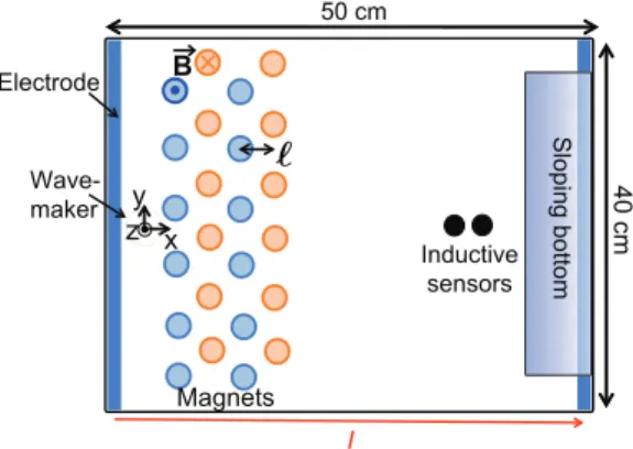
The flow. The device generating the flow is a varia-tion over a previously described setup [5,6]. It is depicted in fig. 1 and consists of a rectangular tank of length 50 cm and width 40 cm. It contains H = 1 cm of Galinstan, be-low a layer of 8 cm of slightly acidified water that limits the oxidation of the Galinstan surface. Galinstan is a liquid al-loy at room temperature made of gallium, indium and tin. It has a density ρ = 6440 kg · m−3and a kinematic
viscos-ity ν = 3.73 × 10⁻⁷m2· s−1. The fluid is stirred
electro-magnetically: four parallel stripes of permanent magnets are placed below the tank. They are aligned along y and distant of ℓ = 31.3 mm, the dipolar axis of the magnets being along the vertical direction. The magnets of a given stripe have the same polarity, and magnets in neighboring stripes have opposite polarities (see fig. 1). The magnetic-field strength at the bottom of the tank and at the center of a magnet is B0= 0.10 T. The combination of the four
T. Humbert et al.
ℓ
Fig. 1: (Color online) Top-view of the experimental cell, con-taining H = 1 cm of Galinstan below 8 cm of acidified water. Below the cell are four parallel stripes of permanent magnets. The polarity of the magnets is directed along the vertical and alternates between neighboring stripes. A current I runs along xbetween two electrodes placed at the boundaries. Its interac-tion with the magnetic field drives the flow through the acinterac-tion of the Lorentz force. Surface waves are generated near one end of the tank and measured at the other end using inductive sensors.
A current I runs inside the liquid metal, between two elec-trodes placed at the far ends of the tank in the x-direction. Through the action of the Lorentz force, the interaction of the current with the magnetic field drives the fluid mo-tion. Above the stripes of magnets, the Lorentz force is oscillatory in x with a spatial period of 2ℓ, mimicking a Kolmogorov forcing in this region of the tank.
When the intensity I is weak, the flow is laminar, with a geometry similar to that of the Lorentz force. As I increases, this laminar solution becomes unstable. The first instabilities of such a Kolmogorov flow are well doc-umented [7–11]. In fully periodic geometry, and consider-ing that the system can be approximated as a 2D one, the parallel Kolmogorov flow first undergoes a station-ary bifurcation, through which it acquires some depen-dence along y. As I further increases, a Hopf bifurcation leads to a time-dependent flow. To illustrate these various regimes, we have performed numerical simulations of the 2D Navier-Stokes equation inside a square domain [0, D]2
with stress-free boundary conditions, where we force a single Fourier mode sin(8πx/D) sin(πy/D). The motion is damped through standard viscosity ν and linear fric-tion with a fricfric-tion coefficient µ satisfying µ = 50π2ν/D2.
In fig. 2 we show the successive regimes observed as we increase the forcing: laminar base flow, steady bifurca-tion and Hopf bifurcabifurca-tion. The finite-size effects inherent to these simulations and to any experimental tank have been carefully described in ref. [11]: because the system is not invariant to a translation along y anymore, the first stationary bifurcation becomes imperfect, with no well-defined threshold value. By contrast, the Hopf bifurcation remains a “perfect” one, because it breaks time-invariance, which is a true symmetry of the base flow. In the following we therefore focus on this Hopf bifurcation.
The waves. Before using them to perform velocimetry, we characterize the waves on the Galinstan-water inter-face in the absence of mean flow. The wavemaker con-sists in a PVC disk of diameter 38 mm and thickness 8 mm touching the interface. An electromagnetic shaker drives a vertical sinusoidal displacement of the disk. The latter pushes the interface up and down, generating weak waves, of amplitude typically slightly below 1 mm. On the other side of the tank, inductive sensors mounted close to the Galinstan-water interface measure the local wave ampli-tude. These sensors are contactless: they are located a few millimeters above the interface and sense its height remotely. Behind the sensors, a sloping bottom ensures that the incoming waves are damped without reflection (see fig. 1).
In this section we use two inductive sensors. The wave-maker and the two sensors are aligned along the x-axis, the distance between the two sensors being ls= 8.5 mm.
When the waves are on, we extract the phase difference θ between the signals of the two sensors. Provided that ls
is shorter than the wavelength λ, θ is linked to the wave number k by the simple relation θ = kls, or equivalently
λ = 2πls
θ . (1)
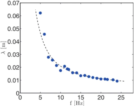
We apply this method to determine the wavelength over the frequency range f ∈ [5, 25] Hz. The corresponding dispersion relation curve is displayed in fig. 3. These data can be compared to the theoretical dispersion relation of gravito-capillary waves: Ω(k)2 =µ ρ − ρ ′ ρ + ρ′gk + σ ρ + ρ′k 3 ¶ tanh(kH), (2) where ρ′ = 1.0 · 103 kg/m3
is the density of water, g is the acceleration of gravity, and σ is the surface tension between Galinstan and water. The latter was determined independently based on measurements of the Faraday in-stability, leading to σ = 0.5 N/m [6]. The theoretical ex-pression (2) is shown as a dashed line in fig. 3 and agrees well with the experimental data. In the following we there-fore use (2) to extract the group velocity of the waves vg= Ω
′
(k), where the prime denotes a derivative with re-spect to k. We finally stress the fact that the finite-depth correction in (2) plays a role only for the lowest frequen-cies visible in fig. 3. For the frequenfrequen-cies considered in the following, the factor tanh(kH) equals unity within 10% and the waves can be considered as deep-water ones.
Surface-wave Doppler velocimetry. – After ap-proximately one day, the interface between the Galinstan and the acidic solution remains clean and deformable, but it appears as a small membrane that hinders any tangen-tial fluid motion at the interface. The properties of this interface then remain stable for weeks before further ox-idation proceeds. We focus on this regime, which allows for clean reproducible measurements over several consec-utive days. The goal is to detect the bifurcations of the
Fig. 2: (Color online) Streamfunction from numerical solutions of the 2D Navier-Stokes equation. Light color is positive and dark color is negative. Increasing the forcing from left to right: laminar solution, steady bifurcation, and oscillatory state shown at two instants separated by half a period. The dashed line in the two last panels symbolizes the wave path over which the velocity is integrated (from left to right) in the present velocimetry method. This integrated velocity oscillates in time: its minimum and maximum values correspond, respectively, to the flows displayed in the third and fourth snapshots.
0 5 10 15 20 25 0 0.01 0.02 0.03 0.04 0.05 0.06 0.07 f[Hz] λ [ m ]
Fig. 3: (Color online) Dispersion relation without mean flow. The blue points correspond to experimental measurements. The dashed line is the theoretical expression (2) with σ = 0.5 N · m−1.
background flow, even though no optical measurements are possible (not even surface particle-tracking velocime-try). In the following we show that the Doppler-shift in-duced by the subsurface flow on the waves can be used as a mean to probe the flow.
We consider only one of the two inductive sensors shown in fig. 1, and we also measure the displacement of the wave-maker. The relative phase difference between the wave amplitude measured at large x and the displacement of the wavemaker is denoted as φ. We extract it using stan-dard Hilbert transform of the two oscillatory signals. We denote as ∆φ(t) the difference in φ when the mean flow is on (I 6= 0) and off (I = 0):
∆φ(t) = φ(t) − φ|I=0. (3)
The fluctuating part of this phase difference is shown in fig. 4 for several values of the current I. For I ≤ 2 A, the phase shift is independent of time. By contrast, for greater values of I, ∆φ depends on time: it is oscillatory, with a period greater than ten seconds and an amplitude that increases with I. We interpret this phenomenon as a consequence of a Hopf bifurcation of the background Kolmogorov flow: the unstable oscillatory mode leads to
0 50 100 −0.2 −0.1 0 0.1 0.2 t[s] ∆ φ ∆ φ [ r a d]
Fig. 4: (Color online) Phase shift ∆φ(t) − h∆φ(t)i as a func-tion of time, where h·i denotes time average, for f = 21.6 Hz. Dashed blue line: I = 2A; Solid line: I = 2.12 A; dash-dotted red line: I = 2.5 A.
a nonzero average fluid velocity along x over the distance of propagation. The cumulative effect of this advecting velocity Doppler-shifts the waves, therefore changing the phase shift φ(t) between the wavemaker and the inductive sensor. The oscillations in ∆φ(t) therefore originate from the oscillations of the background mean flow.
The wave amplitude is below 0.5 mm near the wave-maker, and it is much smaller near the remote inductive sensor because of both viscous damping and radial spread-ing of the wave energy around the wavemaker. A key as-pect of the measurement technique is that it is insensitive to such damping and radial spreading of the wave energy, because the information on the background flow velocity is encoded in the phase of the wave and not in its ampli-tude. We also made sure that the waves do not affect the mean flow, by checking that the signals in fig. 4 are rather insensitive to the wave amplitude: at most, the ampli-tude of oscillation of ∆φ decreases by 20% when the wave amplitude is multiplied by six.
Bifurcation curves. – The present Hopf bifurcation cannot be directly compared to previous experiments or analytical results on Kolmogorov flows, because the lines
T. Humbert et al.
of circular permanent magnets somewhat differ from the standard experimental and theoretical setups. The clos-est experiment may be the one of Michel et al. [10]. In such shallow liquid metal experiments, the main damp-ing mechanism is Hartmann friction near the bottom boundary. In dimensionless form, this phenomenon is quantified by the parameter Rh =pIH/(B0νσL2) (see,
e.g., ref. [12] for details). At the bifurcation threshold, using B0for the typical magnetic-field amplitude, we
ob-tain Rh = 1.0: it lies within a factor of two of the threshold value of the Hopf bifurcation reported by Michel et al. [10], which is acceptable considering the fact that the structure of the forcing strongly differs in the two experi-ments. In the remainder of this section, we characterize in more details the Hopf bifurcation observed in the present experiment.
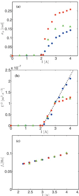
From the time series displayed in fig. 4 we extract the root-mean-square value σφ of ∆φ(t) and plot it as a
func-tion of I in fig. 5(a). The oscillafunc-tion appears above a threshold value of the current I, i.e., above a threshold velocity of the base flow. σφ evolves as the square root of
the departure from onset, in agreement with the standard phenomenology of Hopf bifurcations. We show in fig. 5(c) the frequency of the oscillatory eigenmode, which is also the frequency fo at which the phase difference oscillates.
Of course, waves at different frequencies lead to the same oscillation frequency fo, because they sense the same
os-cillatory eigenmode of the subsurface flow. However, they are not Doppler-shifted by the same phase difference, and the measured value of σφdepends on the frequency of the
surface waves. In the following we elaborate on the precise relationship between the phase shift ∆φ and the subsur-face flow.
Interpretation. – The relation between the phase dif-ference ∆φ(t) and the subsurface flow can be made more quantitative in the limit of scale separation. For a weak depth-dependent flow u(z) directed along x, a standard asymptotic expansion allows one to write the dispersion re-lation of deep-water surface waves propagating along x as ω = Ω(k) + ˜uk, (4) where ω is the wave angular frequency, the function Ω(k) is defined in (2), and only the first correction in u/vg is
retained. The latter correction involves a weighted vertical average of the velocity profile [13]:
˜ u = 2k
Z 0
−∞
e2kzu(z) dz, (5) this expression being valid for a semi-infinite fluid layer occupying z < 0 initially. This approximation holds as long as e−2kH ≪ 1, which is satisfied in the present
ex-periment. We stress the fact that even when partial ox-idation prevents horizontal motions directly at the liquid metal surface, the subsurface flow nevertheless leads to a nonzero value of ˜u in (5) and therefore to a Doppler-shift of the surface waves.
0 1 2 3 4 0 0.05 0.1 0.15 0.2 0.25 (a) I [A] σφ [ r a d] 0 1 2 3 4 0 0.5 1 1.5 2 2.5x 10 −7 (b) I [A] U 2[ m 2. s − 2] 2 2.5 3 3.5 4 4.5 0 0.05 0.1 I [A] fo [H z] (c)
Fig. 5: (Color online) (a) Standard deviation of the phase dif-ference ∆φ(t) as a function of the input current I. (b) The square of the typical velocity U defined in (11) as a function of I. (c) Frequency fo of the oscillations of ∆φ(t) as a function
of I. Blue circles: f = 6 Hz. Green triangles: f = 11 Hz. Red squares: f = 21.7 Hz.
The dispersion relation (4) can be readily extended to a flow u(x, y, z) that depends slowly on x and y as compared to the wavelength. We obtain a relation between the fre-quency and the local wave number k(x) of the waves:
ω = Ω[k(x)] + ˜u(x)k(x), (6) where u denotes the x-component of u and the ˜· denotes the weighted vertical average (5). In the present setup the wave frequency is imposed by the wavemaker and we write ω = ω0= const. By contrast, the local wave number k(x)
adapts to the local fluid velocity. We denote as k0 this
wave number in the absence of mean flow, such that ω0=
from k0and we can expand (6) to first order in k(x) − k0,
which yields
ω0= Ω(k0) + Ω ′
(k0)[k(x) − k0] + ˜u(x) k0. (7)
Denoting as vg= Ω′(k0) the group velocity of the waves in
the absence of currents, we obtain the local wave number
k(x) = k0 µ 1 −u(x)˜ vg ¶ . (8)
The wavenumber being the local gradient of the phase, we integrate this relation to get
φ = k0 Z x=L x=0 · 1 −u(x)˜ vg ¸ dx, (9)
where x = 0 denotes the position of the wavemaker and x = L = 0.34 m the position of the inductive sensor. Sub-tracting the same expression for ˜u = 0, we finally obtain
∆φ = −k0 Z x=L x=0 ˜ u(x) vg dx. (10)
Because the travel time of the waves between emitter and receiver is much faster than the timescale of the mean flow evolution, we can use eq. (10) at any time to compute the phase shift ∆φ(t) due to the slowly evolving mean flow, substituting in (10) the instantaneous velocity ˜u(x, t).
Equation (10) provides a direct connection between the phase difference and the subsurface flow: we estimate ˜u by defining the typical sensed velocity as
U = vgλσφ
2πL . (11) In fig. 5(b), we plot U2
as a function of I. In the vicin-ity of the bifurcation threshold, this representation leads to a good collapse of the data obtained for different wave frequencies, which indicates that U defined in (11) is in-deed the right order parameter. This collapse also con-firms that the wave amplitude is irrelevant provided one stays in the linear regime: the weak waves do not affect the background flow. The collapse remains satisfactory even for the lowest wave frequency, f = 6 Hz, for which there is no real scale separation between the wavelength λ and the typical scale 2ℓ of the flow. This may come from the fact that the small-scale velocity fluctuations (visible in the numerical snapshots 2) cancel each other in expres-sion (10). Only the larger-scale velocity structures leading to a nonzero cumulative average when integrated over x contribute to (10), and these structures indeed have a large typical scale as compared to λ.
Equation (11) also provides an order of magnitude of the sensitivity of the surface-wave Doppler velocimetry method. In fig. 4, we show a rather clean oscillation sig-nal measured in the immediate vicinity of the bifurcation threshold (I = 2.12 A). The corresponding typical veloc-ity is U ≃ 1 · 10−5
m · s−1
. Although unknown geometrical
prefactors may affect the relationship between U and the true velocity, this low value indicates a remarkable sensi-tivity of the measurement technique, making it competi-tive as compared to available velocimetry methods for the low-velocity regime of liquid metal hydrodynamics.
Conclusion. – We have presented an original velocime-try technique where the Doppler-shift of surface waves is used to detect the subsurface flow. It is particularly well suited to detect small velocities in liquid metals, where partial oxidation and pollution of the surface prevent the use of standard optical methods such as surface particle-tracking velocimetry. As an example of such an appli-cation, we precisely measured the first Hopf bifurcation of a Kolmogorov flow of Galinstan. In the limit of scale separation between the wavelength and the lengthscale of the flow, we established the direct connection between the subsurface flow and the measured phase shift. This led to a good collapse of the data obtained at various wave frequencies. Another possible application of this method would be to detect mean flows under complex surface-wave fields. Indeed, surface particle tracking is then strongly perturbed by the Stokes drift of the surface waves, and PIV is difficult if the particles are to be imaged through the deformed free surface. If the waves are linear, one can externally superimpose to the complex wave field a well-controlled monochromatic wave and detect the mean flow through a lock-in detection of the phase difference between the emitter and a remote sensor. In any case, the advan-tages of the present method are its ease of implementation and accuracy: it efficiently detects weak velocity signals in free-surface flows. Of course, the method also has limita-tions, one of which being that the measurement integrates the velocity along the path between the wave emitter and receiver, leading to a rather nonlocal measurement. An exciting next step would be to combine several emitters and receivers to image the mean flow through surface-wave tomography.
∗ ∗ ∗
We thank V. Padilla for building the experimental setup. This research is supported by Labex PALM ANR-10-LABX-0039 and ANR Turbulon 12-BS04-0005.
REFERENCES
[1] Shercliff J. A., The Theory of Electromagnetic Flow-Measurement (Cambridge University Press) 1987. [2] Eckert S., Buchenau D., Gerbeth G., Stefani F.
and Wiess F.-P., J. Nucl. Sci. Technol., 48 (2011) 490. [3] Herault J., P´etr´elis F. and Fauve S., EPL, 111
(2015) 44002.
[4] Ricou R. and Vives C., Int. J. Heat Mass Transfer, 25 (1982) 1579.
[5] Guti´errez P. and Aumaˆıtre S., Eur. J. Mech. B/Fluids, 60 (2016) 24.
T. Humbert et al.
[6] Guti´errez P.and Aumaˆıtre S., Phys. Fluids, 28 (2016) 025107.
[7] Bodarenko N. F., Gak M. Z. and Dolzhansky F. V., Izv. Akad. Nauk (Fiz. Atmos. Okeana), 15 (1979) 1017. [8] Thess A., Phys. Fluids A, 4 (1992) 1385.
[9] J¨uttner B., Marteau D., Tabeling P.and Thess A., Phys. Rev. E, 55 (1997) 5479.
[10] Michel G., Herault J., P´etr´elis F. and Fauve S., EPL, 115 (2016) 64004.
[11] Tithof J., Suri B., Pallantla R. K., Grigoriev R. O.and Schatz M. F., J. Fluid Mech., 128 (2017) 837. [12] Sommeria J., J. Fluid Mech., 170 (1986) 139.
[13] Stewart R. H. and Joy J. W., Deep Sea Res. Oceanogr. Abstr., 21 (1974) 1039.