3-D groundwater modeling at regional scale

3-D groundwater modeling at regional scale

Francesco Kimmeier1_{, Mahmoud Bouzelboudjen}1_,

László Király1 1

CHYN - Centre d'Hydrogéologie, Université de Neuchâtel, Emile-Argand 11, 2007 Neuchâtel, Suisse

ABSTRACT

Large hydrogeological basins are constituted of several superimposed aquifers, separated by geological formations of relatively low permeabilities. The delimitation of the different flow systems is far more difficult to realize for a heterogeneous system. Flux vectors provide valuable indications about groundwater flow paths and hydraulic exchanges between the different geological formations. Hydraulic relationships between two superimposed aquifers can vary locally: an aquifer can «feed» the underlying one at some point and conversely elsewhere. These relationships, which constitute in fact the flow field, will be determined by the structure of the basin as defined by the spatial distribution of the rock permeabilities, and by the boundary conditions, as defined by the locations of the recharge and discharge areas. The aim of this study is to show schematically the deep groundwater flow patterns between the massives of the Aar and the Black Forest. The hydrogeological profiles illustrate three-dimensional flow fields inside a large volume of terrain and represent but one of the numerous solutions of the mathematical modelling realized. Computations have been performed for a steady state flow regime, which means that the boundary conditions do not vary with time.

On the basis of modelling results, it was possible to illustrate schematically the deep flow systems of the most important aquifers between the Aar massives and the Black Forest (Malm, Muschelkalk and upper Cristallin). An approximate but plausible representation of the groundwater circulation in deep aquifers was obtained thanks to the model. We are able to distinguish between the hydraulic relationships of two superimposed aquifers in various regions. The three-dimensional representation shows the outcrop zones of the different geological formations as well as the situation of recharge areas, which are characterised by high potentials, and discharge zones, which are characterised by low potentials in valleys represented by the hydrographic network.

Modelling results are then compared to available measurements in an attempt to validate the results. It is interesting to notice that it was possible, to a certain extent, to verify the modelling results by deep drillings. Most particularly, measurements of the hydraulic potentials at various depths in these boreholes have revealed upwellings close to the regional discharge areas.

Keywords : Hydrogeology, groundwater modeling, 3-D finite elements, Waste

repository, Validation, Switzerland

1. INTRODUCTION

Groundwater flow patterns in the subsurface of the Swiss Plateau are illustrated schematically (Annex 1-6). The main difficulty in representing graphically such patterns lies in the fact that groundwater flows in a three-dimensional space. In order to facilitate the reader’s understanding, the main directions of flow are represented in vertical profiles and on maps (plane view) showing the lateral extension of some of the most important aquifers.

The term validation have been applied by various researchers to indicate how well a model approximates reality. This term is used to describe the ability of a mathematical model to describe a physical system (e.g., the appropriateness of Darcy's law to describe groundwater flow in a porous or fractured media) and the ability of a conceptual model to reproduce the observed conditions ("reality").

Validation of hydrogeologic conceptual models is difficult. This is due to the large number of degrees of freedom in the model (e.g., permeability distribution in space and applied boundary conditions) and the sparsity of available information with which to compare the simulated results. As a result, several models can be formulated which adequately explain the available data. In addition, it is difficult to rule out the possibility that a single measurement may only be representative of very local hydrogeologic conditions which are impossible to incorporate in large scale models. Given these difficulties, the validation part will describe the results of attempts to validate the conceptual models of ground-water flow in northern Switzerland.

2. THE SYSTEM OF GROUNDWATER FLOW

Water can be found in pores and fissures down to a depth of several thousands of metres below sea level: this water is called groundwater. Groundwater (Fig. 1) flows from recharge areas, which are generally situated in elevated areas, towards discharge zones, which mainly correspond to the hydrographic system of lakes, streams and valleys. The average direction of groundwater flow is represented schematically by flowlines or flow fields. This direction as well as the velocity of groundwater flow is expressed in the simplest case by Darcy’s law (cf. «Definitions»).

Figure 1 : Recharge and discharge areas from Skinner & al. [1991]

Soil Aquifer Aquitard

Groundwater flow system Alimentation

Free aquifer surface Flow direction; resident time: 1) days

2) years 3) decades 4) centuries 5) millenia

DEFINITIONS

 Equipotentials are lines (two-dimensional case) or surfaces (three-dimensional case) linking points with same hydraulic potential.

 Defined at any point "A" of the aquifer, hydraulic potential is the sum of the altitude of this point above a reference level and of the water height corresponding to the groundwater pressure at this same point. The hydraulic potential is not equal to the groundwater pressure at point "A".

 Hydraulic gradient is a vector that is perpendicular to the equipotentials at any points of the aquifer.

 Flux vector is the product of the hydraulic gradient by the permeability or the hydraulic conductivity of the aquifer (Darcy's law).

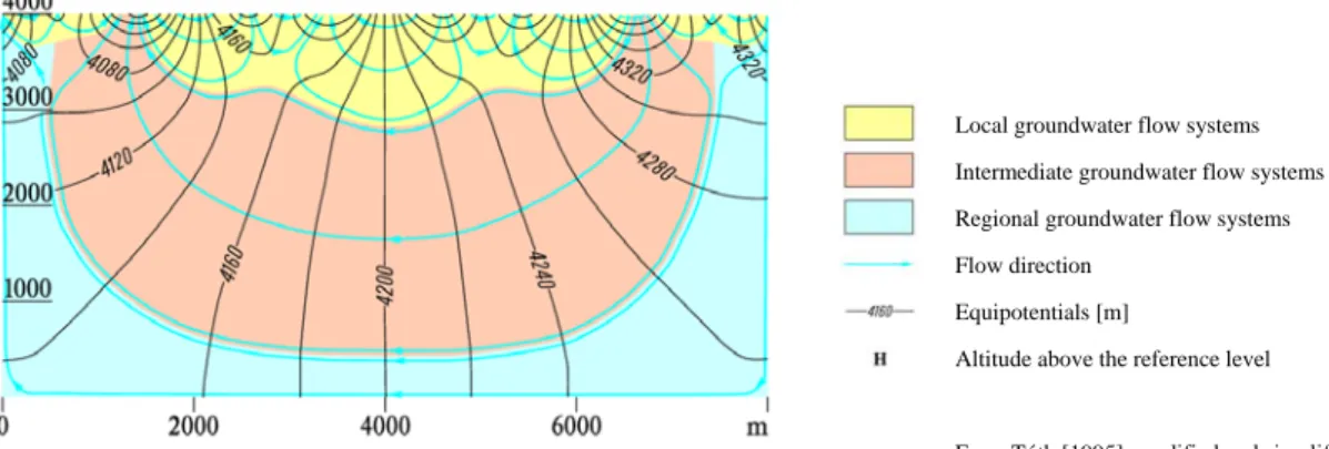
According to theoretical studies by Tóth [1963, 1995], flowlines represent the local, intermediate or regional flow systems that exist between recharge and discharge areas (see Fig. 2, which shows different flow systems within a theoretical, homogeneous hydrogeological basin). One can understand intuitively that flow systems represent an ideal framework to study the thermal, chemical and isotopic properties of groundwater. Even an approximate knowledge of these properties can provide valuable information (even if it is qualitative) about the possible transport of

dissolved substances in groundwater at various depths (e.g. as a result of rock-water interactions). Figure 2 shows that the location of sources of dissolved substances with respect to local, intermediate or regional flow systems is an essential component to understand the distribution of dissolved substances within the aquifer. Moreover, it is important to notice that the hierarchic structure of flow systems results from the hierarchic structure of the hydrographic network, or, more precisely, of the discharge zones.

Direct measurements of the directions of groundwater flow at any point of the earth’s crust are largely impossible. This means that flow fields need to be inferred in most cases by indirect methods, such as mathematical modelling.

Figure 2 : Sketch plan of the groundwater flow systems

Local groundwater flow systems Intermediate groundwater flow systems Regional groundwater flow systems Flow direction

Equipotentials [m]

Altitude above the reference level

Principle of "finite elements" mathematical model:

The flow region is subdivided into "finite elements" with a relatively simple geometry (see sketch-plan), each element being defined by the position of a number of nodes (points on the edges). In assigning at each element a permeability and a storage coefficient and by integrating the differential equation on each element one obtains as much linear equation that there are nodes in the model (generally between 1'000 and 200'000). By solving the equation system [Király, 1985] one computes for each node either the hydraulic potential (where the flux is imposed) or the in or out flux (where the potential is imposed). Potential or flux imposed values are called "boundary conditions". Without imposing boundary conditions it is impossible to simulate the groundwater flow.

3. GROUNDWATER FLOW IN LARGE HETEROGENEOUS

BASINS

Large hydrogeological basins are constituted of several superimposed aquifers, separated by geological formations of relatively low permeabilities. The delimitation of the different flow systems is far more difficult to realize for a heterogeneous system than for a homogeneous case as represented in figure 2; however, flux vectors provide valuable indications about groundwater flow paths and hydraulic exchanges between the different geological formations. Hydraulic relationships between two superimposed aquifers can vary locally: an aquifer can «feed» the underlying one at some point and conversely elsewhere. These relationships, which constitute in fact the flow field, will be determined by the structure of the basin as defined by the spatial distribution of the rock permeabilities [Király, 1970], and by the boundary conditions, as defined by the locations of the recharge and discharge areas.

Theoretical two-dimensional cases allow for an easier understanding of flow systems and their usefulness in the case of hydrogeological studies [Bouzelboudjen, 1993], but it would be even more important to obtain a wider knowledge about three-dimensional flow patterns in real aquifers and find out how to reconstruct and represent them in real systems.

4. GROUNDWATER FLOW BETWEEN THE AAR AND THE

BLACK FOREST MASSIFS

The hydrogeological profiles presented here illustrate in a schematic way groundwater flow in the subsurface of the Swiss Plateau, between the massifs of the Aar and the Black Forest [Bouzelboudjen & al., 1997]. Such profiles illustrate three-dimensional flow fields inside a large volume of terrain and represent but one of the numerous solutions (cf. Legend - Annex 2) of the mathematical modelling realized in an earlier study [Kimmeier & al., 1985].

The representation of flow fields is quite easy for theoretical two-dimensional cases, because flow vectors do not have a component perpendicular to the plane of representation. This is not the case for real systems of large dimensions, because it is practically impossible to find a plane of representation that would not be oblique to the vectors of flux, at some point or other. Furthermore, aquifers whose thicknesses are small relative to their lateral extent, for example a few metres compared to several hundred kilometres, are particularly difficult to represent either as block diagrams or as vertical profiles. We have therefore decided to present the results by projecting the vectors of flux onto straight vertical profiles, or onto maps corresponding to the lateral extension of some particularly important aquifers. This requires more attention from the reader, because a component of flow perpendicular to the plane of representation is associated to each vector. Transferring the real system to a hydrogeological model requires several simplifications of the geometry of the principal geological formations and the hydrogeological boundary conditions chosen to set the limits of the model.

The regional model used as the base for the hydrogeological profiles presented here is limited by the Aar Massif in the south and the Black Forest in the north; the Constance Lake represents the eastern boundary and the Aare river is used as the western limit. The lateral boundaries chosen for the model correspond to the limits of the regional flow systems which can reach considerable depths (the Rhine, Rhône and Aare valleys). The initial goal of this model was to study deep flow systems within the crystalline basement of the northern part of Switzerland [Kimmeier & al., 1985, Nagra, 1988, Thury & al., 1994, Voborny & al., 1992]. The upper boundary of the model represents the surface of the unconfined water table. It has been estimated by means of hydrogeological and topographical maps (three-dimensional representation). Hydrogeological conditions at the boundaries are based upon observed values of hydraulic potentials or flow rates (infiltration, exfiltration), or upon estimations. Such conditions represent in each case the hypotheses that have been introduced into the model. Subsequently, the coherence of these data will have to be verified by an analysis of the modelling results. The schematic block diagram (cf. Annex 2) shows the simplified geological data and the three-dimensional reconstruction of the geometry of the formations as they were modelled.

Computations have been performed for a steady state flow regime, which means that the boundary conditions do not vary with time. The program FEM301 and FEN's code family [Király, 1985, 1998] has been used to compute the field of hydraulic potentials and flow rates in the modelled area. Modelling results are then compared to available measurements [see point 6]. It is interesting to notice that it was possible, to a certain extent, to verify the modelling results by deep drillings. Most particularly, measurements of the hydraulic potentials at various depths in these boreholes have revealed upwellings close to the regional discharge areas [Hufschmied & al., 1989]. On the basis of modelling results, it was possible to illustrate schematically the deep flow systems of the most important aquifers between the Aar Massif and the Black Forest. An approximate but plausible representation of the groundwater circulation in deep aquifers was obtained thanks to the model. For this particular case [Bouzelboudjen & al., 1997] we used the computer code FEN [Király, 1997] derived from FEM301. We are able to distinguish between the hydraulic relationships of two superimposed aquifers in various regions (cf. profiles - Annex 4), as demonstrated for theoretical cases (cf. Fig. 1 and 2).

The three-dimensional representation shows the outcrop zones of the different geological formations as well as the situation of recharge areas, which are

characterised by high potentials, and discharge zones, which are characterised by low potentials in valleys represented by the hydrographic network.

Profile 3, which is approximately perpendicular to the other profiles, shows the local groundwater flow systems. Such systems constitute the main discharge zones in the bottoms of valleys and provide the predominant vertical fluxes in those regions.

5. GROUNDWATER FLOW SYSTEMS IN THE CRYSTALLINE

BASEMENT, THE MUSCHELKALK AND THE MALM

AQUIFERS

Both as an illustration and example of groundwater circulation, three major Swiss aquifers are described: the crystalline basement, the Muschelkalk and the Malm. Flow conditions in the crystalline basement (Annex 6) and Malm (Annex 5) aquifers are illustrated by means of two maps.

The Malm aquifer play an important role within the deep groundwater circulation of the basin. Recharge areas are located at South (outcrop area on the tridimensional representation) and groundwaters flow towards regional discharge areas located at North (Constance region on Annex 5 and Aar region on profile 2).

The recharge and discharge zones of the Muschelkalk aquifer correspond to outcrop zones, which are the Alps in the south and the tabular Jura in the north, according to the three-dimensional representation. Because it is impossible to illustrate the results as profiles at this scale, we confine ourselves to making the following comment: In the Alps, groundwater from the Muschelkalk flows into the high valleys of the Aare, the Reuss and the Rhine rivers, as well as into the region of Vättis. In the north, groundwater discharges into the Rhine valley between Basel and Bad Säckingen, then into the Wutach valley. Between both areas, the upper part of the Muschelkalk aquifer is drained by downcutting valleys, such as the Sisslen, the Aare and the Rhine valleys.

Recharge areas of the upper part of the alterated Cristallin are located in the Aar and Black Forest massifs (see tridimensional representation). As the formations that overlay the upper part of the Cristallin are very few permeable, the alimentation of this geological serie can not occur outside of these two mentionned regions. Therefore, discharge occurs in surface at low points where Cristallin outcrops that is in the valleys (profile 1 - Annex 4). In the Alps, discharge is possible mainly in the upper course of the Aar, Reuss, Rhine, Linth rivers as well as in the "fenêtre de Vättis". In the Black Forest, discharge occurs in the Wiese, Dreisam and Rhine valley between Säckingen and Tiengen. Profile 2 (Annex 4) show that the waters coming from South flow under the Jura and flow into the Rhine valley. This discharge area constitues a limit separating the regional groundwater flow systems coming from South and North. In North-West part, groundwater of the Cristallin leave the modelised zone (Neunberg am Rhein/Ilfurth sector). Under the molassic basin, flow patterns in the Cristallin are quite parallel until the main Jura overlapping. As one approach the South-North watershed, vertical fluxes in the non alterated part of the Cristallin become important (profile 2 north of Olten). In the region near of the Rhine valley discharge the upper part of the alterated Cristallin drains the other parts of the Cristallin weakly alterated (profile 2, region of Rheinfelden). Profile 2 puts in evidence the role of the Rhine valley as regional discharge area.

6. MODEL VALIDATION

In order to validate the regional model 6 NAGRA boreholes, Water wells and Oil/Gas borings data at the North of Switzerland were used (see Fig 3) [Andrews & al., 1996].

The hydrogeologic conceptual model should be validated to the extent feasible prior to using the results from such a model for predictions of repository performance. This validation may take several forms. At a scale of kilometers or tens of kilometers, the model should be able to reproduce the general ground-water flow directions and overall volumetric flow rates within and between the various transmissive hydrogeologic units. At a scale of meters or tens of meters one would like the model to predict the travel path(s) and velocities of dissolved radionuclides which may escape the engineered containment facility. Validation of the travel path(s) and velocities is virtually impossible without extensive in-situ testing and in fact, there will always be some residual uncertainty in defining the precise flow path. However, validation of the general flow regime is possible using the following observations:

 potentiometric data volumetric  discharge rates

 infiltration rates  bulk geochemistry

 isotopic (stable and radioactive) geochemistry  temperature

While each of these observations has an associated uncertainty, combining them should yield a consistent "picture' of the ground-water flow system. A brief summary of the status of the efforts to validate the regional groundwater flow model in northern Switzerland is described below.

Potentiometric Data

The observed potentiometric data of the deep aquifers in the study region is presented in Kimmeier & al. [1985]. Numerous additional data exist for the shallow

Figure 3: NAGRA (Nationale Genossenschaft für die Lagerung Radioaktiver Abfälle) study area and deep exploratory borings

alluvial aquifers, but as the heads in these aquifers essentially mimic the surface topography they are not considered here. Of the 80 wells in the study area, 14 are completed in the crystalline. In some cases, the wells are open over several formations, hence a mixed head is measured. In other cases, numerous tests have been performed in a single formation within an individual well. This is particularly true of the testing performed by NAGRA in the crystalline at Böttstein, Weiach, Schafisheim, Kaisten and Leuggern.

Measured heads are subject to many uncertainties. The potential error associated with heads measured by short term pressure tests is discussed by Grisak and Pickens [1985]. Additional errors exist in the data from the oil industry (generally drill stem tests) and from thermal and mineral water wells where the exact test conditions are often not known or well construction, test procedures, or borehole pressure history effects may impact the measured head. For these reasons the reported heads should only be considered accurate to within plus or minus 10 m, with this error being up to several tens of meters for many of the wells in the study region.

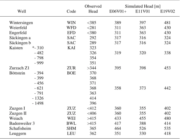
Comparison of observed and simulated heads in the crystalline for three regional model runs is presented in Table 1. Run E06V0I and EllV0l differ principally by the

Table 1: Comparison of Observed and Simulated Heads within the Crystalline

Observed Simulated Head [m]

Well Code Head E06V01+ E11V01 E19V02

Wintersingen WIN <385 389 397 481 Weierfeld WFD <281 311 363 430 Engerfeld EFD <380 311 363 430 Säckingen a SAC 292 317 316 324 Säckingen b SAC 289 317 316 324 Kaisten *- 310 KAI 323 - 482 326 319 320 338 - 798 354 - 999 351 Zurzach Z1 ZUR >344 395 398 453 Böttstein - 394 BOE 370 - 399 368 - 456 371 - 621 368 358 373 442 - 791 363 - 1326 414 - 1498 396 Zuzgen I ZUZ <412 360 355 402 Zuzgen II ZUZ <406 360 355 402 Weiach WEI >415 433 455 480 Badenweiler 3 BWL >415 417 388 414 Schafisheim SHM 365 464 526 535 Leuggern LEU 362 351 330 418

*-310: Indicated the depth (m) + see text

permeability of the uppermost aquifers in the Alps. Run E19V02 utilized prescribed infiltration rates as opposed to a prescribed head boundary condition. With the exception of Schafisheim the agreement between observed and simulated heads is

generally quite favorable. It has been suggested [Kimmeier & al., 1985] that the low head measured in the crystalline at Schafisheim is due to a short circuit through the confining sedimentary strata.

Volumetric Discharge Rates

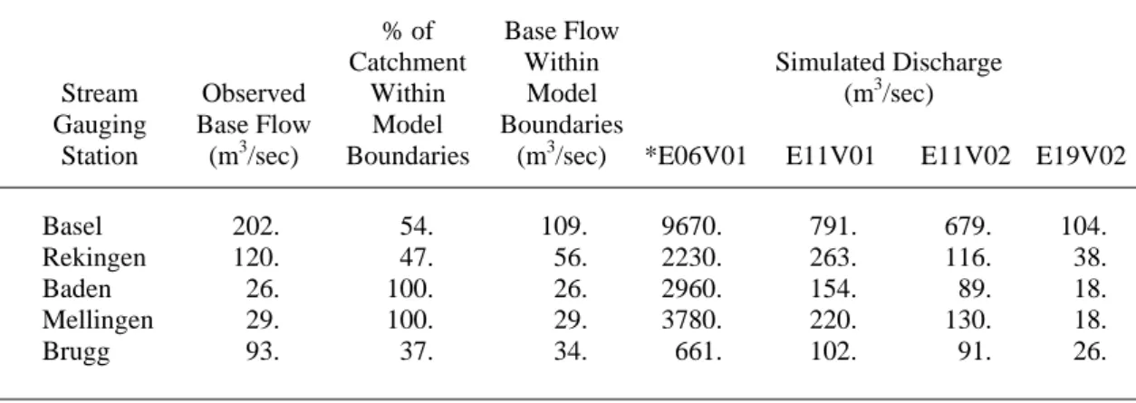
The volumetric discharge rates calculated along all modeled rivers are compared to observed base level stream flows at five gauging stations (Table 2). We assume that the lowest observed stream flow is totally supplied by groundwater discharge as opposed to surface runoff. In both run E06V01 and EllV0l the water table surface is prescribed. Therefore decreasing the permeability of the uppermost aquifer in the Alps (run EllV0l) decreases the recharge and discharge. Run E11V02 differs from EllV0l in that the prescribed heads in the Alpine recharge areas are decreased by 500 m, causing a reduction in recharge and discharge. Run E19V02 utilizes prescribed infiltration rates which have been adjusted to better approximate the observed discharges [Kimmeier & al., 1985]. It is interesting to note that, while applying infiltration rates improves the fit between observed and simulated stream discharges (Table 2), the fit worsens between the observed and simulated heads in the area of interest (Table 1). This reinforces the decoupled nature of the shallow and deep ground-water flow regimes.

The ability to directly compare observed and simulated groundwater discharges as a means of model validation must be treated with caution. First, the observed base flow may be controlled by the alluvial aquifers not the deeper sedimentary or crystalline aquifers. Second, the simulated discharge is almost totally a function of the permeability and gradients in the outcropping aquifers, not the relatively small fluxes in the deeper confined aquifers. Finally, the degree of averaging incorporated in the model implies that small drainage systems which do contribute to the observed discharges are not explicitly modeled. In summary, it is difficult to place a great deal of confidence in the comparison of observed and simulated discharge rates as a validation tool. It does indicate if the model is order of magnitude correct but nothing more precise. It should be noted that detailed water balance assessments over small areas also aid little due to the averaging required in the models.

Table 2: Comparison of Observed and Simulated Stream Discharge % of Base Flow

Catchment Within Simulated Discharge Stream Observed Within Model (m3/sec)

Gauging Base Flow Model Boundaries

Station (m3/sec) Boundaries (m3/sec) *E06V01 E11V01 E11V02 E19V02

Basel 202. 54. 109. 9670. 791. 679. 104. Rekingen 120. 47. 56. 2230. 263. 116. 38. Baden 26. 100. 26. 2960. 154. 89. 18. Mellingen 29. 100. 29. 3780. 220. 130. 18. Brugg 93. 37. 34. 661. 102. 91. 26. * See text

Infiltration Rates/Water Table Surface

The boundary condition on the upper surface of a ground-water flow model may be either a prescribed infiltration rate or a specified head. If the infiltration rate is assigned, the simulated water table may be compared to the observed water table to ensure some degree of compatibility. If the water table surface is specified, the calculated infiltration rates may be compared to observed recharge rates to again check the validity of a particular simulation. Because in both cases the results are strongly controlled by the permeability of the uppermost element, any differences between observed and simulated near-surface heads or infiltration rates is just as likely due to permeability uncertainty as it is to the prescribed boundary condition.

Only a qualitative significance can be placed on the comparison of observed and simulated near-surface hydrogeology. First, there are no direct observations of infiltration rates in Switzerland. Even if there were, they would only represent very local conditions which would be impossible to extrapolate given the variable geology, topography, meteorology and vegetation. Secondly, there are no direct observation of heads in the recharge areas. We may assume these heads mimic the surface topography, but to what extent is difficult to define (especially in the Alps).

In summary, great care must be utilized in attempting to validate a large scale hydrogeologic model by the use of near-surface observations. Even if a good "match"

is obtained, this implies very little with regards to the deep groundwater flow regime which is of greatest interest. The approach taken in [Kimmeier & al., 1985] has been to vary the upper boundary conditions to evaluate their impact on the deep flow system of interest.

Bulk Geochemistry

The spatial variability of the dissolved constituents in groundwater can be used to provide qualitative statements concerning the general groundwater flow directions. The following conclusions have been made by Schmassmann and others [1984]:

1. If one assumes the salinities observed in the crystalline at Schafisheim (about 8 g/l) are representative of crystalline groundwaters south of the Permo-Carboniferous trough, then the low salinities (1 to 2 g/l) observed at Kaisten, Böttstein (upper 500 m) and Leuggern imply recharge from the north (Figure 4).

2. Gypsum saturation variations within groundwaters of the Upper Muschelkalk

indicate a generally south to north component of flow in the region between the Lägern and the Rhine.

These observations have been used to insure that the general flow regime simulated by the model agrees with the geochemistry (compare Annex 5 and Fig. 4). However, as observed geochemical differences can often be the result of local hydrogeologic conditions (for example mixing of different formation waters) some care must be utilized in interpreted regional flow regimes from only geochemical evidence.

Isotopic Geochemistry

Pearson [1985] has concluded from his evaluation of the isotopic data from Böttstein that:

1. the residence time of the Muschelkalk groundwater is 17'000 years (± 6'000

years) based on corrected C-14 and

2. the residence times of C-14 in the Buntsandstein/Upper crystalline groundwater

range between 6'000 and 12'000 years.

Great care must be utilized in the interpretation of "residence times" generated from isotopic measurements due to the effects of possible geochemical reactions, matrix diffusion, or channeling on measured groundwater "ages". In addition, given the wide variability in the permeability and flow porosity along a likely travel path from the recharge area to the measurement point, it is impossible to utilize groundwater "ages" to unambiguously validate the results of a hydrodynamic model. Given these precautions, the above ages are at least consistent with the results of the regional and local hydrogeologic models [Kimmeier & al., 1985].

Temperature Distribution

The groundwater temperature may also provide some indication of the flow regime. A severe limitation with temperature (as is also the case with reactive tracers), however, is the non-conservative nature of its transport. The measured temperature at any point, whether a spring or a well, is strongly controlled by the thermal properties of the rock mass. Except in extremely rapidly flowing groundwater systems, the observed temperature is more a function of the conductive transfer of heat through the rock than the convective flow of heat with the water.

Anomalous temperatures do exist in the study region. In particular, the thermal springs at Baden (in the Muschelkalk) have a temperature of about 47 °C. This

indicates the discharging water at Baden must come from great depths. The probable source of this water is from the south where the Muschelkalk is much deeper (and hence warmer). This south to north flow in the Muschelkalk has been reproduced in the regional model [Kimmeier & al., 1985].

Some conclusions for groundwater model validation

While the initial effort to validate the regional hydrogeologic model is encouraging, the work is not complete. As additional data are being collected and interpreted (esp. hydrochemical, isotopic, thermal, and hydrogeologic) this study must be treated as preliminary.

At the present stage in the characterization of the groundwater flow regime, sensitivity analysis is an important component in safety analysis. The impact of uncertain parameters on the ability to validate the conceptual model and on the predicted ground-water flow paths and flow rates must be considered. These sensitivity analyses are reported on in Kimmeier & al. [1985].

7. REFERENCES

Andrews R.-W., Kimmeier F., Perrochet P., Király L., 1986. Validation of

hydrogeologic models to describe groundwater flow in the Crystalline basement of Northern Switzerland. Mat. Res. Soc. Symp. Proc., Vol. 50, 1985, p.107-114.

Materials Research Society, Pittsburgh, Pennsylvania, USA. Scientific Basis for Nuclear Waste Management IX, Editor Lars O. Werme.

Bouzelboudjen, M. 1993. Cartographie hydrogéologique et systèmes d’écoulement

souterrain. Centre d’hydrogéologie de l’Université de Neuchâtel – Service

hydrologique et géologique national. Rapport inédit, Berne.

Bouzelboudjen M., Király L., Kimmeier F., Zwahlen F. 1997. Représentation

schématique des écoulements souterrains en Suisse. Profils hydrogéologiques issus de modèles mathématiques 3-D à éléments finis. Planche 8.3 de l'Atlas

Hydrologique de la Suisse. Institut de Géographie de l'Université de Berne, Office Fédéral de la Topographie et service Hydrologique et Géologique National, Berne, Suisse.

Grisak, G., Pickens, J.F., 1985. Hydrogeological Testing of Crystalline Rocks during

the NAGRA Deep Drilling Program. NTB 85-08, NAGRA, Baden, Switzerland.

Hufschmied, P., Frieg, B. 1989. Observation of hydraulic heads in the Nagra

boreholes in Northern Switzerland. Nagra Bulletin, Special Edition 39-49, Baden.

Király, L. 1970. L’influence de l’hétérogénéité et de l’anisotropie de la perméabilité

sur les systèmes d’écoulement. In: Bulletin der Vereinigung schweizerischer

Petroleumgeologen und -ingenieure, 37/91:50–57, Zürich.

Király, L. 1985. FEM301 – A three-dimensional model for groundwater flow

simulation. Nagra Technischer Bericht NTB 84-49, Baden.

Király L., 1998. FEN's code family (Finite Element Neuchâtel) - Three Dimensional

Model for Groundwater Flow and Transport Simulation Codes (VAX-VMS,

Kimmeier, F. & al. 1985. Simulation par modèle mathématique des écoulements

souterrains entre les Alpes et la Forêt Noire; Partie A: Modèle régional, Partie B: Modèle local (Nord de la Suisse). Nagra Technischer Bericht NTB 84-50, Baden.

Nagra 1988. Sedimentstudie – Zwischenbericht 1988. Möglichkeiten zur Endlagerung

langlebiger radioaktiver Abfälle in den Sedimenten der Schweiz. Nagra

Technischer Bericht NTB 88-25, Baden.

Pearson, F. J. Jr., 1985. Sondierbohrung Böttstein-Results of Hydrochemical

Investigations: Analysis and Interpretation, NTB 85-05, NAGRA, Baden,

Switzerland.

Skinner, B.J., Porter, S.C. 1991. The dynamic earth: an introduction to physical

geology. Second edition, New York.

Schmassmann, H., Balderer, W., Kanz, W., Pekdeger, A., 1984. Beschaffenheit der

Tiefengrundwasser in der Zentralen Nordschweiz und den Angrenzenden Gebieten,

NTB 84-21, NAGRA, Baden, Switzerland.

Thury, M. & al., 1994. Geology and Hydrogeology of the Crystalline Basement of

Northern Switzerland. Synthesis of Regional Investigations 1981–1993 within the

Nagra Radioactive Waste Disposal Program. Nagra Technischer Bericht NTB 93-01, Baden.

Tóth, J. 1963. A Theoretical Analysis of Groundwater Flow in Small Drainage

Basins. Jour. of Geoph. Research, Vol 68, N° 16, pp 4795-4812.

Tóth, J. 1995. Hydraulic continuity in large sedimentary basins. In: Hydrogeology Journal Volume 3, Nr. 4/1995:4–16, Hannover.

Voborny, O. & al., 1992. Analysis of regional groundwater flow in crystalline rocks

of Northern Switzerland: Results of a numerical model using an equivalent porous medium. Nagra Interner Bericht, Baden.

Situation of the three-dimensional model Streams of the model

Faults and overthrusts of the model Profiles situation

Annex 3 : Three-dimensional representation of the simulated grounwater flow [Bouzelboudjen & al, 1997]. Horizontal scale 1: 800'000

Simulated equipotential [m] Surface of the free aquifer (See Annex 4)

Flow direction

Arrow lenght corresponds To the logarithm of the Flux vector

Flow direction Arrow lenght corresponds to the logarithm of the flux vector

Annex 6 : Simulated hydraulic potentials at the upper limit of the Crystalline [Bouzelboudjen & al., 1997]

Flow direction Arrow lenght corresponds to the logarithm of the flux vector

Annex 5 : Simulated hydraulic potentials at the upper limit of the Malm [Bouzelboudjen & al., 1997]