Application of Bayesian-based uncertainty and global sensitivity analyses to spacecraft thermal design

Application of Bayesian-based Uncertainty and

Global Sensitivity Analyses to Spacecraft Thermal

Design

by

Conor B. McMenamin

B.S., Mechanical Engineering

Northeastern University (2012)

Submitted to the Department of Aeronautics and Astronautics

in partial fulfillment of the requirements for the degree of

A

Master of Science in Aeronautics and Astronautics

at the

MASSACHUSETTS INSTITUTE OF TECHNOLOGY

June 2016

@

Massachusetts Institute of Technology 2016. All rights reserved.

A uthor ...

Certified by...

Signature redacted

Department of Aeronautics and Astronautics

M~y42 016

Signature redacted

Rebecca A. Masterson

Research Engineer, Department of Aeronautics and Astronautics

Thesis Supervisor

Certified by ...

Accepted by ...

Signature redacted

Richard P. Binzel

Professor of Planetary Science

Joint Professor of Aeronautics and Astronautics

E\

Thesis Supervisor

Signature redacted

I

Paulo C. Lozano

Associate Professor of Aeronautics and Astronautics

Chairman, Graduate Program Committee

OF T1HN0WGY

JUN

28 2016

IBRARIES

ARCHIVES

Application of Bayesian-based Uncertainty and Global

Sensitivity Analyses to Spacecraft Thermal Design

by

Conor B. McMenamin

Submitted to the Department of Aeronautics and Astronautics on May 19, 2016, in partial fulfillment of the

requirements for the degree of

Master of Science in Aeronautics and Astronautics

Abstract

As satellite design has increased in complexity, the evolution of thermal engineering of spacecraft has plateaued. For years, thermal engineers have used the same principles of designing to stacked worst case scenarios and applying additional margin on top of the already conservative predictions. Recent publications have proposed the use of Bayesian-based propabilistic tools in the design of spacecraft in the effort to avoid overly conservative thermal designs. An issue with utilizing these tools is the typically high computational cost associated with traditional thermal modeling. To help bridge the gap from state-of-the-art to industry standard, this thesis develops a methodology to reduce simulation time and implement these analysis techniques in the industry standard software, Cullimore & Ring Technologies Inc., Thermal Desktop. These design methods are applied to the REgolith X-ray Imaging Spectrometer (REXIS), a student built x-ray spectrometer aboard NASA's OSIRIS-REx mission. Uncertainty analysis shows the area of the main instrument's radiator could have been reduced

by 11%, as compared to the design obtained from conventional techniques, and still

have a 99% probability of meeting the thermal requirements in all mission phases. Furthermore, global sensitivity analysis results provide insight into the thermal design of the instrument which could have been used to avoid anomalies experienced during integration and testing. Overall, results show that previously established analysis techniques scale to more complex thermal systems and the insights gained from these methodologies can significantly reduce thermal overdesign.

Thesis Supervisor: Rebecca A. Masterson

Title: Research Engineer, Department of Aeronautics and Astronautics Thesis Supervisor: Richard P. Binzel

Title: Professor of Planetary Science

Disclaimer: This material is based upon work supported by the United States Air

Force under Air Force Contract No. FA8721-05-C-0002 and/or FA8702-15-D-0001. Any opinions, findings, and conclusions or recommendations expressed in this material are those of the author and do not necessarily reflect the views of the

Acknowledgments

First and foremost, I would like to thank the MIT Lincoln Laboratory Lincoln Scholars Program for sponsoring my graduate education. Furthermore, I am thankful to my group leaders at MIT Lincoln Laboratory, Dr. Keith Doyle and Mark Bury, for supporting me through the Lincoln Scholars Program application and while I was away at school.

I thank all my fellow REXIS team members. Thanks to David Carte, Mike Jones, James Chen, Kevin Stout, and Pronoy Biswas. I would like to specially thank Mark Chodas and Laura Bayley. Mark, you are an amazing systems engineer and REXIS is lucky to have you. Laura, thank you for all of the help with class and coding. Without you two, I would not have been able to make it through to the end.

Thank you to my advisors, Professor Richard Binzel and Dr. Becky Masterson, for your guidance on this thesis and my time here at MIT.

Last, but not least, thank you to all of my friends and family who supported me through these tough two years. Thank you Mom and Dad for being there for me and supporting me through all of my endeavors. Thank you to all of my friends who were there to help me de-stress after tough days and celebrate the good days. Thank you Jenn for taking care of me during this last thesis push and keeping me sane throughout the past two years.

Contents

1 Introduction 17

1.1 Background and Motivation . . . . 18

1.1.1 Spacecraft Thermal Control System . . . . 18

1.1.2 Uncertainty in Thermal Design . . . . 22

1.2 Bayesian Approach to Thermal Design . . . . 26

1.2.1 Bayesian Uncertainty Background . . . . 27

1.2.2 Uncertainty Analysis . . . . 28

1.2.3 Global Sensitivity Analysis . . . . 30

1.2.4 Review of Recent Research and Research Goals . . . . 31

1.3 Thesis Roadmap . . . . 32

2 REXIS Background/Overview

2.1 REXIS Mission Overview ... 2.2 REXIS Thermal Overview ...

2.2.1 REXIS Instrument Description ...

2.2.2 REXIS Mission Thermal Overview ...

2.2.3 REXIS Thermal Requirements ... 2.3 Spectrometer Thermal Design Overview ...

2.3.1 Thermal Zone 1: Electronics Box ...

2.3.2 Thermal Zone 2: Tower and Titanium Thermal Isolation Layer

2.3.3 Thermal Zone 3: CCDs and Radiator . . . . 2.3.4 Thermal Zone 4: Radiation Cover and Cover Deployment Mech-anism . . . . 35 35 37 38 40 42 44 45 46 47 50

2.4 SXM Thermal Design Overview ... 52 3 Design Methodology & REXIS Solar X-ray Monitor (SXM) Case

Study

3.1 Design Methodology ... ...

3.1.1 Uncertainty Analysis Methodology . . . .

3.1.2 Global Sensitivity Analysis Methodology .

3.1.3 Implementation in Thermal Desktop . . .

3.2 SXM Design Results . . . .

3.2.1 Problem Definition . . . .

3.2.2 Uncertainty Analysis . . . . 3.2.3 Global Sensitivity Analysis . . . . 3.3 Lessons Learned . . . . 3.3.1 Global Sensitivity Analysis Convergence .

3.3.2 Thermal Desktop Specific Lessons Learned

3.4 Bayesian-based Design Implementation

4 Spacecraft Battery Case Study 4.1 Problem Definition ...

4.2 Uncertainty Analysis ... ...

4.3 Global Sensitivity Analysis Results . . . .

5 REXIS Spectrometer Case Study

5.1 Problem Definition . . . . 5.2 Surrogate Model Creation . . . . 5.3 Uncertainty Analysis . . . .

5.4 Global Sensitivity Analysis . . . .

5.5 Frangibolt Thermal Vacuum Testing Anomaly . . . .

6 Conclusion

6.1 Thesis Summary . . . . 6.2 Applicability of Bayesian-based Design Methodology . . . .

55 . . . . . 55 . . . . . 56 57 . . . . . 59 . .... 63 . . . . . 63 64 . . . . . 66 . . . . . 69 . . . . . 69 . .... 71 . . . . 72 75 75 79 81 85 85 88 92 94 96 103 103 105

List of Figures

1-1 MIL-STD-1540E recommended analysis and test margin . . . . 23 1-2 TIRS instrument radiatior with MLI covering ~60% of the surface area

[1 . . . . 25

1-3 Integrated laser transmitter instrument radiator on the CALIPSO

satel-lite [21 . . . . 26

1-4 Comparison of analysis predictions to in flight temperatures [31 . . . . 27 1-5 Probability density functions representing differing states of knowledge 28 1-6 Thesis roadmap . . . . 32

2-1 OSIRIS-REx with Sample Acquisition Arm Extended [4] . . . . 36

2-2 Views of REXIS Spectrometer and SXM mounted on OSIRIS-REx [5J 38

2-3 REXIS Spectrometer and SXM shown with major components labeled 39

2-4 OSIRIS-REx Mission Solar Environment [6] . . . . 41

2-5 REXIS Spectrometer four thermal zones . . . . 44 2-6 Cross sectional view of thermal zone 1: Electronics box . . . . 46

2-7 Wedgelock used for conductive thermal path from PCB to electronics box w alls . . . . 47 2-8 Titanium and Torlon Thermal Isolation Layers (TIL) . . . . 48 2-9 Detailed views of thermal zone 3: CCDs and radiator . . . . 49 2-10 TiNi FD04 Frangibolt actuator

[71

and detailed mid plane view of

fran-gibolt and radiation cover deployment mechanism . . . . 50 2-11 Radiation cover heaters and thermostats . . . . 51

3-1 Thermal Desktop Methodology flow chart . . . . 60 3-2 Example output code used to write Thermal Desktop QoI output to

text file . . . . 62 3-3 SXM thermal model created in Thermal Desktop . . . . 65 3-4 Probability of meeting SXM thermal requirements versus temperature

of TORE, based on 50,000 Monte Carlo samples of the uncertain system 67

3-5 Comparison of global sensitivity analysis results of the main effect Sobol' indices of the SXM for the SDD and SEB QoIs. The parameter variable names are defined in Table 3.1. . . . . 68 3-6 Plots of Sobol' indices convergence calculation versus amount of model

evaluations for the SXM's SEB and SDD QoIs . . . . 70 3-7 Plots of Sobol' indices convergence calculation versus amount of model

evaluations for two separate SXM SEB QoI calculations . . . . 71 3-8 Comparison of global sensitivity analysis results of the main effect

Sobol' indices for different SEB QoIs. The parameter variable names

are defined in Table 5.1. . . . . 73

3-9 Flow chart of Bayesian-based design methodology, including Thermal D esktop . . . . 74

4-1 Thermal model of spacecraft battery with component details . . . . . 76 4-2 Surrogate thermal model of battery with radiation conductor . . . . . 81 4-3 Probability of meeting spacecraft battery thermal requirement versus

radiator size based on 10,000 Monte Carlo samples of the uncertain system . . . . 82 4-4 Global sensitivity analysis results of the main effect Sobol' indices of

the spacecraft battery. The parameter variable names are defined in

Table 4.2. . . . . 83

4-5 Updated global sensitivity analysis results of the main effect Sobol' indices of the spacecraft battery. The parameter variable names are

5-1 REXIS Spectrometer Thermal Desktop model . . . . 86 5-2 Full Spectrometer thermal model with surrogate spacecraft thermal

m odel . . . . 90 5-3 Radiation conductor to space node, used to represent uncertain

emis-sivity of radiator . . . . 91 5-4 Probability of meeting Spectrometer thermal requirements versus

ra-diator size based on 10,000 Monte Carlo samples of the uncertain system 93 5-5 Global sensitivity analysis results of the main effect Sobol' indices of

the Spectrometer CCDs and Frangibolt QoIs. The parameter variable names are defined in Table 5.1. . . . . 95 5-6 Spectrometer mounted in the thermal vacuum chamber . . . . 97 5-7 Temperature of the frangibolt housing, radiation cover, and tower for

the duration of the REXIS flight TVAC test . . . . 98

5-8 Radiation cover with frangibolt installed prior to TVAC testing . . . 99

5-9 Comparison between model predicted radiation cover heater duty cycle with actual test results . . . . 99 5-10 Comparison between updated model predicted radiation cover heater

duty cycle with lower Gf and actual test results . . . . 100 5-11 Radiation cover post TVAC test after cover actuation has taken place

List of Tables

1.1 Recommended max and min environmental heat loads for satellites in

low Earth orbit . . . . 20

2.1 OSIRIS-REx payload instruments and descriptions . . . . 36

2.2 REXIS driving thermal mission cases . . . . 41

2.3 Spectrometer and SXM temperature requirements/QoIs per compo-nent in C . . . . 42

3.1 SXM thermal model uncertain inputs descriptions, density profiles, max, min, and nominal values . . . . 65

4.1 Spacecraft battery Qol thermal requirements in C . . . . 76

4.2 Uncertain inputs of spacecraft battery . . . . 78

5.1 Uncertain inputs of Spectrometer . . . . 89

5.2 Correlation results between surrogate Spectrometer and spacecraft model with full Spectrometer and spacecraft model in C . . . . 91

5.3 Comparison of averaged steady state temperatures between the EM correlated thermal model, updated thermal model, and flight TVAC test results . . . . 101

Chapter

1

Introduction

Satellite designs are becoming more complex as advanced technology has made its way to the spacecraft market [8]. As spacecraft design has been evolving to incorporate the state-of-the-art complexities, the design and implementation of thermal solutions to meet these ever changing challenges has plateaued. Spacecraft technologies are becoming smaller and lighter, but dissipate the same, if not more, heat. As the com-ponent heat densities have increased, the methods used to design a thermal solution by analyzing to the stacked worst case with additional margin has remained the indus-try standard. Thermal engineers in indusindus-try are understandably risk adverse because of the lack of precise system knowledge during the design phase and the conservative nature of spacecraft design in general [9]. This design approach ensures the thermal requirements of the system are met, but puts undue stress on the other subsystems, schedule, and overall budget [9]. Not all of the thermal overdesign is derived from the thermal engineer's conservatism. Many of the thermal modeling and design decisions originate from a lack of system knowledge. Lack of precise knowledge may manifest itself in the uncertainty of the thermal design parameters or in the uncertainty from the still in-process design of the other subsystems. For example, conservatism can be applied to estimate a thermal control surface's end-of-life (EOL) thermo-optical prop-erty. Conversely, a safety factor can/should be applied to the power output from the power system engineer's estimation of heat from a still in design avionics subsystem. This thesis seeks to build upon recent efforts to use each thermal parameter's state

of knowledge in the thermal design, in a probabilistic Bayesian context, as opposed to designing to an unrealistic stacked worst case. Within this proposed design frame-work, the thermal engineer can gain more insight into the system to appropriately and systematically apply margin and resources. More specifically, this thesis endeavors to bridge the gap between state-of-the-art and industry standard by showing how these tools and design perspective can be implemented on real, computationally intensive, spacecraft applications in the industry standard software.

1.1

Background and Motivation

This section begins with a brief overview of thermal engineering in the aerospace industry. The thermal engineer's role and responsibilities are discussed in order to give context for the case studies presented in later chapters. A major piece of the thermal engineer's role is the design, implementation, and test of the spacecraft's thermal control system (TCS). A description of the TCS is given, along with an overview of the parameters that affect the design of the TCS. Finally, this section presents a discussion on the industry standard practice of applying margin to the TCS and how that margin affects the spacecraft TCS and the satellite as a whole system.

1.1.1

Spacecraft Thermal Control System

Before beginning a discussion on different thermal control systems, it is important to understand why a TCS is needed at all for satellites. Space is a difficult environ-ment to thermally control electronics as the absence of air means the only modes of heat transfer are conduction and radiation. These two modes of heat transfer are represented by Equations 1.1 and 1.2, respectively, where k is conductivity, A is area,

AT ttet

Ky represents the thermal gradients, E is emissivity, or is the Stefan-Boltzmann con-stant, and T and T2 are temperatures of radiatively interacting components. All of

the thermal energy entering,

Qi,

and leaving the system,

QOu,

must be balanced through these two heat transfer modes alone, as shown in Equation 1.3.

AT

Qradiation = EAso(T - T2 4)

(1.2)

Qin = Qout (1.3)

Heat entering the system is broken up into 1) environmental heat loads and 2) self generated heat. Environmental heat loads consist of solar flux, planetary reflected solar flux (albedo), or planetary infrared (IR) heat (planetshine). Solar flux and albedo both transfer heat through thermal radiation in the solar wavelengths. Plan-etshine is the transfer of heat from the planetary body to the orbiting satellite via thermal radiation in the infrared wavelength. For Earth orbiting satellites, all three of these heat loads vary naturally because Earth's slightly elliptical orbit around the sun marginally increases or decreases the solar distance. Solar radiation is propor-tional to distance from the sun, as shown in Equation 1.4. As the Earth reaches its perihelion, solar flux, and therefore albedo and planetshine increase. The opposite is true for Earth's aphelion. Solar flux, QSolarFlux, can also vary due to increased or decreased solar activity.

QSolarFlux oC 1/r2 (1.4)

Independent of solar flux variations, albedo naturally varies because various parts of Earth reflect different amounts of solar energy. Deserts naturally have a higher reflectivity than oceans or forests but both of these reflectances can change depending on the presence or absence of higher-reflectance clouds. To encompass all of the bounding minimum and maximum environmental heat load cases, NASA published Table 1.1 which shows the recommended ranges for each heat load for low Earth orbit

(LEO) satellites [10].

Self generated heat enters the system from the waste heat produced by the opera-tion of electronics. Electronics are never 100% efficient and these inefficiencies cause

- a

Table 1.1: Recommended nax and min environmental heat loads for satellites in low Earth orbit

Solar Constant (W/m2) Albedo Factor Planetshine (W/m2)

0.25 256 Nominal 1368 0.30 239 0.35 222 0.25 267 Winter Solstice 1422 0.30 249 0.35 231 0.25 247 Summer Solstice 1318 0.30 231 0.35 214

heat to be dissipated inside the spacecraft. The self generated heat varies as a func-tion of spacecraft operafunc-tions. For example, iii a typical spacecraft more internal heat generation occurs during a high power communications pass than during a low power charging scenario. All of these heat loads comprise the heat entering the system Qi, as shown in Equation 1.5.

Qzn QSolarFlux + QAlbedo + QPlanetshine + QInternalDissipations (1.5)

All of the heat leaving the system, Qaut, leaves through thermal radiation of spacecraft exterior surfaces.

It is the thermal engineer's responsibility to design a TCS that can appropriately reject the environmental and self generated heat while keeping spacecraft components within their operating temperature ranges. The most common tools to control the heat entering and leaving the system are passive thermal control systems (PTCS). Passive thermal control mechanisms are preferred for a TCS due to their simplicity and low size, weight, and power (SWaP). Multi-layer insulation (MLI), radiators, and thermnal straps are common examples of passive thermal control devices. Multi-layer insulation is a fundamental PTCS tool used on alhmost every satellite. MLI consists of many layers of aluminized mylar with outer layers of kapton. The result of stacking these layers provides a set of thermal radiative resistors in series with one another.

These thermal resistors create a very low effective emissivity through the MLI, turn-ing the blanket into a thermal insulator. This effective thermal insulator prevents heat from entering the system from the environment and also prevents heat from leaving the spacecraft. Radiators are typically used to reject heat to the environment in a controlled way. Radiators are usually designed with a surface coating with a low absorptivity a and high emissivity E. The high & ensures the radiator can reject heat effectively while the low a reduces the amount of solar environmental flux the radiator absorbs. Sizing the radiator properly is an important task for the thermal engineer. A radiator designed too small will cause the electronics to run hot. Con-versely, a radiator that is oversized means the spacecraft will need extra heater power to warm up the electronics, putting an unnecessary strain on the electrical power sub-system. Passive thermal control also includes the intentional conductive coupling or isolating of components. High conductivity thermal straps are used to intentionally conductively couple two components that are far away and need to be structurally decoupled. If isolation is desired, low conductivity materials like titanium or GlO can be used to conductively isolate components [11, 12].

If passive thermal control devices are not adequate to meet the thermal needs of the spacecraft, active thermal control systems (ATCS) can be used. Heaters, thermo-electric coolers (TECs), and fluid loop heat pipes are common examples of active thermal control devices. Heaters convert electrical energy into heat to warm up cold subassemblies in a spacecraft. Conversely, TECs use electricity to create a heat flux between two metals. This heat flux creates a cooling effect which reduces the temperature of one of the metals. TECs are typically used to cool sensitive imagers. Heat pipes use a self contained two phase fluid loop cycle that efficiently transports heat from a hot surface to a cold surface. ATCS gives the thermal engineer more control over spacecraft temperatures but comes at the price of electricity in the case of heaters and TECs and design complexity for the heat pipes [11, 12]. For more information on spacecraft thermal control systems, see Gilmore [111.

1.1.2

Uncertainty in Thermal Design

An important role of the thermal engineer in the design of the TCS is the identification of and designing for uncertainty in the system. The varying levels of environmental heat loads is shown in Table 1.1. PTCS mechanisms in particular have high uncer-tainties. For example, the effective emissivity of the MLI, commonly referred to as the blanket's e* (e-star), changes depending on how many layers are in the MLI and on whether the blanket is small or large, flat or uneven, and if it contains dacron meshing or embossed mylar for layer to layer spacing. The higher the E*, the more

heat the MLI allows to flow through it. For radiators or other thermal control sur-faces, the thermo-optical properties typically degrade over the mission life. Radiation darkening, outgassing contamination, and atomic oxygen erosion can all cause the surfaces absorptivity to rise, increasing the amount of heat entering the system from the environment. Bolted joint thermal interface resistances have variability based on the size of the bolt used, materials bolted together, and the torque used. All of these uncertainties need to be accounted for in the thermal design to ensure the TCS will keep the spacecraft components within their operational or survival temperature ranges.

To deal with these uncertainties, thermal engineers analyze and design to the stacked worst case hot and cold scenarios. Each uncertain parameter's high or low bound is either associated with a hot or cold case. For example lower, solar flux, minimum spacecraft internal power dissipation, and beginning of life (BOL) thermo-optical properties all drive the spacecraft temperatures lower, creating a cold scenario. A stacked worst case is when all uncertain parameters are chosen with either their associated bounding hot or cold values all at once. If the TCS can meet the thermal requirements under these stacked worst case hot and cold conditions, the design is adequate for all of the more realistic scenarios in between the stacked worst cases.

On top of the stacked worst case results, thermal engineers apply temperature margin. Thermal margin is applied to both the design and testing of components. Figure 1-1 shows the recommended analysis and test margins from military standard

Design +71 'C Maximum +66-C Predicted Temperature +61 C

~]~~11

/ / Thermal Jncertainty Margin Minimum -243C Predicted Temperature I11C or -29 -C 25% control 340C authority Test Qualification 10 Hot ---Protoqual Hot Qualification

Acceptance Hot Margin (1OC

- --- -- ---- -- --- --Acceptance Protoqual Margin Margin (5CC) -- ---- ----Acceptance d Qualificatior Protoqual Cold Margin (10 C

CUa a on

Cold

Figure 1-1: MIL-STD-1540E recommended analysis and test margin

MIL-STD-1540 [13]. As shown in Figure 1-1, the standard recommends 110C of analysis margin on top of the 100C of Qualification testing margin. Therefore, if the analysis results predict component operational temperatures of -13'C to 50'C in the stacked worst cases, the component would need to be able to operate at -34'C to 71'C. If this wide temperature range is unacceptably high for a component, TCS design changes like increasing radiator size need to be implemented to reduce the maximum temperature predictions. Margin is also applied to ATCS mechanisms by oversizing the heating or cooling capacity of the device. For example, the General Environmental Verification Standard (GEVS) (GSFC-STD-7000) recommends that in the stacked worst case cold scenario, at minimum spacecraft voltage where a heater is producing its minimal amount of heat, the heater shall be oversized such that it operates at less than 70% duty cycle [14]. The 70% heater duty cycle increases the current draw of the circuit by 40% but allows the thermal engineer to only keep 50C of analysis margin.

Designing the thermal control system to the stacked worst case scenarios and 23

Model Temp. Predictions

adding additional analysis and test margin on top of these predicted temperature extremes do ensure the satellite will not violate allowable temperatures limits, but these design and margin allocation practices lead to overdesign. The stacked worst case scenarios produce predicted temperature extremes but no consideration is given to the likelihood or frequency of the conditions aligning in flight as analyzed [151. These maximum temperature predictions are not normalized by their occurrence du-ration predicted on orbit. Often, temperature predictions that occur transiently on orbit, even on the order of minutes, are reported as predicted mission worst case temperatures. These components are then tested at elevated temperatures at steady state even though a short transient temperature excursion is more likely to produce graceful degradation rather than catastrophic failure [151.

Overdesigned systems occur in industry because of these conventional practices of designing to a stacked worst case and adding additional margin. Figure 1-2 pro-vides an extreme example of the results from an overdesigned system. The Thermal Infrared Sensor (TIRS) instrument on the Landsat Data Continuity Mission is a cryogenic instrument that was designed on an aggressive schedule [16]. Because of this tight schedule, design decisions were made to accomodate lead time instead of optimization of the system. With this built up conservatism, the thermal vacuum (TVAC) test results concluded that the radiator was oversized. After TVAC testing, 60% of radiator area was covered with MLI to prevent overcooling of the instrument on orbit [161. Given the unusually aggressive schedule and the 40-50% design margin recommendations for cryogenic systems [171, the overdesigned radiator is not com-pletely unexpected. The schedule and margin notwithstanding, the extra radiator area directly adds mass to the system, but also has the secondary affect of increasing the mass of the structure supporting the radiator.

The TIRS instrument is an extreme example of thermal overdesign but a more typical illustration is given by the Integrated Laser Transmitter (ILT) LIDAR instru-ment, shown in Figure 1-3, on the CALIPSO satellite. The ILT is designed with an integrated radiator to bias the instrument cold and separate survival and opera-tional heater circuits to warm up the lasers. The radiator size is designed to meet

Figure 1-2: TIRS instrument radiatior with MLI covering ~60% of the surface area

[1]

the thermal requirements for a stacked worst hot case. For the cold cases, the instru-ment has a 50 W survival heater and a 20 W operational heater to get the laser to operational temperature range before lasing. During satellite-level TVAC testing, it was discovered that power dissipation was lower than expected, and the operational heater was inadequate to overcome the cooling effects of the radiator. Post TVAC it was determined that the radiator area was overdesigned by 21.5% [18]. To address this overcooling issue, the CALIPSO team decided not to cover part of the radiator area with MLI, and instead use both the operational and survival heaters simulta-neously to warm up the lasers enough for operation. With this heater solution, the overdesigned radiator means not only extra mass, but also extra power draw from the electrical power subsystem.

Although the TIRS and CALIPSO cases show thermal overdesign, it is important to evaluate the effectiveness of thermal control system designs over a broader range of missions. Studying four radiator designs on the LRO, GPM, and ATLAS mis-sions, Garrison concluded that adding 5'C of analysis margin can increase radiator sizing by up to 8% and survival heater power by up to 20% [3]. Since this analysis

margin is shown to have such an impact on the overall system, it is important to determine whether this conventional practice of margin allocation is necessary. In

or I

Figure 1-3: Integrated laser transmitter instrument radiator on the CALIPSO satellite

[2]

practice, radiators are typically used to control the temperature of spacecraft elec-tronics. Figure 1-4 shows a histogram of the difference between predicted hot stacked worst case temperature extremes and temperatures observed on orbit for the elec-tronics of six NASA missions launched from 2001 to 2010. In the figure, Quadrant I shows the percentage of mission life where the on orbit temperatures are greater than the predicts, and Quadrant II shows when the observed temperatures are less than the predicts. Based on the distribution from the figure, traditional modeling practices produce models that are overly conservative. Most model predicts are over 100C hotter than the observed on orbit temperatures, meaning the thermal system is designed to an unrealistically conservative case [3]. Therefore, better understand-ing of model uncertainties can help reduce the overdesign of satellite thermal control systems.

1.2

Bayesian Approach to Thermal Design

An alternative approach to the conservative conventional design methodology in-corporates Bayesian-based uncertainty and global sensitivity analyses, examples of which include recent publications by Stout [5] and Thunnissen [19]. Section 1.1 dis-cusses the classic conventional approach to thermal design. Evidence is presented that shows room for improvement over designing to a stacked worst case and adding

Actual > Predicts --- ) Predicts >Actual

Quadrant I

Quadrant Il

10 -I 0 20 30 40 U. AQUA -AURA -GLAST -LRO -- SDO SWIFT -OVERALL 60

Predicted - Observed Max Temperatures (deg C)

Figure 1-4: Comparison of analysis predictions to in flight temperatures [3]

significant margin on top of the already conservative results. This section presents a Bayesian design approach to help reduce the overdesign caused by conventional tech-niques. Bayesian concepts are briefly discussed and these concepts are compared to the conventional framework. Bayesian-based uncertainty analysis and global sensitiv-ity analysis are introduced to show how application of these analyses aides spacecraft thermal design. Finally, the section concludes with a review of recent research in this area and an outline of the thesis contributions, including addressing and solving difficulties in implementation.

1.2.1

Bayesian Uncertainty Background

Before discussing the application of a Bayesian framework to the design of a spacecraft TCS, it is important to have some background on Bayesian probability and how this framework differs from the convention. In industry, thermal engineers generally follow a frequentist probability methodology. In frequentist probability, the uncertain parameters are fixed at constant values. The parameter information is obtained by taking the average of repeated tests'.

In Bayesian probability, the uncertain parameters are unknown and described 27

1 1 0.8- 0.8-'F 0.6 -- 0.6-0.4 0.4-0 0 0.2- 0.2-0 0 0 2 4 6 8 10 0 2 4 6 8 10 z z

(a) Good state of knowledge, low variance (b) Poor state of knowledge, high variance

Figure 1-5: Probability density functions representing differing states of knowledge

probabilistically as continuous probability density functions (PDF). The test results are fixed instead of the parameters. The parameter distributions are updated using the test results'. These PDFs probabilistically describe the parameter, including a more accurate representation of the mean and variance. The mean and variance of the PDFs represent the possible range of the parameter as well as the state of knowledge of the parameter. A state of knowledge is how well the parameter is known or understood. For example, a very well known parameter would have a PDF similar to Figure 1-5a, while a very uncertain parameter may be better represented by Figure 1-5b.

1.2.2

Uncertainty Analysis

As discussed in Section 1.1.2, many of the important parameters that affect the tem-peratures in a TCS naturally vary. Uncertainty analysis is a typical technique that is used to calculate the variance in the model output. Model output is any informa-tion produced by the results of a simulainforma-tion. For example, typical model output for 'Casella, George. "Bayesian and Frequentists." ACCP 37th Annual Meeting, Philadelphia, PA. Department of Statistics, University of Florida.

thermal models consists of temperatures and heat fluxes. Thermal requirements intro-duced in Section 1.1 are the component temperature criteria that a TCS is designed to satisfy. Model output that maps directly to tile requirements of the system are called Quantities of Interests (Qol). Typical QoIs in the thermal design of spacecraft are battery temperatures, temperatures of sensitive imaging devices, and maximum temperatures of electronic boards. Typically, uncertainty analysis is not performed

on all of the model output, but just the critical QoIs.

Applying Bayesian-based uncertainty analysis to the spacecraft thermal design gives the thermal engineer more information earlier on in the design process to help reduce thermal overdesign. For most of the uncertain input parameters, the thermal engineer has good knowledge of the typical average and extremes over which these modeling inputs fall. In creation of the hot and cold stacked worst cases, the thermal engineer ignores the most likely value (average), and instead chooses to evaluate the model with one of the values from either extreme. The other extreme for each parameter is then chosen and the model is reevaluated for the other stacked worst case. This conventional mindset produces two discrete outputs for the thermal engineer to evaluate with no information on the likelihood of either case actually happening in flight. In a Bayesian model, each uncertain input parameter has a unique PDF and model evaluations produce a continuous PDF output. Uncertainty analysis is performed on this Bayesian-based thermal model by propagating the uncertainty through the system by monte carlo sampling the uncertain parameters according to their distributions. These model evaluations produce a continuous distribution of model outcome [201. The continuous model output includes all of the ranges of possible solutions and probabilities associated with each solution. The two stacked worst case scenarios are represented in the continuous PDF output, but probabilities are associated with these scenarios so the thermal engineer can properly weight them in the design process. This continuous distribution of model output provides the thermal engineer with more information about the design, so that they can apply margin in a system specific manner to help reduce overdesign.

1.2.3

Global Sensitivity Analysis

Global sensitivity analysis (GSA) is a quantitative way for the thermal engineer to gain insight into the effects of the uncertain model parameters. Sensitivity analysis has long been a way for system designers to understand the relative importance of pa-rameter inputs in determining the model output [20, 21, 221. This analysis is useful for determining which parameters significantly affect the solution and which parameters have a small, if any, affect on the model output. Engineers then use these param-eter sensitivities to make more informed decisions on the system design. Typically, sensitivity analysis is performed using calculus-based approaches. A calculus-based approach takes the derivative of the model output Y versus a parameter input Xj,

&Y/9Xi. This approach is not optimal because uncertain parameter variances, in

a Bayesian context, are not taken into account, and the engineer needs to decide where to take the derivative, which can induce errors or local maximums or minu-mums. Therefore, derivatives are only informative at the location selected and do not provide information on the rest of the model output space created by the uncertain parameter inputs [20, 22].

Variance-based global sensitivity analysis provides a solution that overcomes the shortfalls of calculus-based methods. Variance-based GSA decomposes the model variance so that portions of the variance are assigned to each uncertain input model parameter. The input model parameters are then investigated to determine how much each parameter contributes to the total variance of the output. The GSA methodology is particularly effective because it captures the effects of the full range of each input parameter, and is able to show the effects of parameter interactions [201. Variance-based GSA is a natural follow on to uncertainty analysis because uncertainty analysis calculates the variance in the QoI, while GSA provides the answer to which parameters are causing the most amount of variance. Furthermore, the input parameters for GSA are already defined by a continuous PDF, with a mean and finite variance. The conventional thermal engineering approach is not viable for this GSA technique because the discrete inputs of the stacked worst case analyses create discrete outputs

without variance. Since this GSA technique uses the output variance to perform the sensitivity analysis, the technique is not applicable to a model that does not produce an output without a variance.

1.2.4

Review of Recent Research and Research Goals

This thesis seeks to build upon recent work of applying state-of-the-art uncertainty analysis and global sensitivity analysis to spacecraft thermal systems. This thesis does not attempt to create new numerical techniques, but applies these well proven methods to spacecraft thermal design. Moreover, recent research has been published by Stout [51 and Thunnissen [191 that investigates the applicability of Bayesian-based thermal modeling. Stout and Thunnissen have proven the feasibility, but there are research gaps that need to be reconciled before a transition to industry. Stout's Ph.D. works through uncertainty analysis and variance-based global sensitivity analysis on a thermal model, but does so utilizing a thermal model created in Matlab. Matlab is a powerful engineering tool but is not the industry standard that thermal engineers use for their thermal modeling. The aerospace industry standard thermal software is Cullimore & Ring's Thermal Desktop, which provides a graphical environment for thermal engineers to use the SINDA solver. Thunnissen, on the other hand, does use a SINDA based thermal model for his work, but does not perform a variance-based global sensitivity analysis.

It is important to resolve these research gaps before thermal engineers perform uncertainty and global sensitivity analyses in practice because the time involved to learn new software or implement the methodology as is would be prohibitively long. Thermal Desktop has become the industry standard for good reasons. The software neatly wraps together geometry creation, surface ray tracing, and the power of the well-used SINDA solver all together. Creating a large spacecraft thermal model in Matlab is too time consuming and prone to significant errors. The reason variance-based GSA is not the industry standard is not only because of the use of discrete stacked worst cases, but also because of the high computational cost 1201. Using variance-based GSA in practice, 104 model evaluations can be required to estimate the

sensitivity of one input with an uncertainty of 10% 123J. When one model evaluation can take upwards of hours, 104 model evaluations seems impossible. Because of this high computational cost, it is important to develop techniques to reduce run times before thermal engineers in industry caii implement this methodology.

1.3

Thesis Roadmap

Chapter 3

Methodology/SXM Case Study Chapter 1

Background and MotivationBtrCsSu

Chapter4

Spacecraft Battery Case Study ChapterCt

REXIS Overview

Chapter5

Spectrometer Case Study

Case Studies

Figure 1-6: Thesis roadmap

This thesis is organized into five chapters. Figure 1-6 shows the thesis roadmap. Chapter 1 is the thesis introduction, including background, motivation, literature re-view, and thesis goals. Chapter 2 provides an overview of the REgolith X-ray limag-ing Spectrometer (REXIS) instrument, a student built x-ray spectrometer aboard NASA's OSIRIS-REx mission, which is the case study for Chapters 3 and 5. Chapter 3 explains the methodology used to accomplish the thesis goals of bringing the tech-niques into tile industry standard software and reducing mnodel run times. To ensure the imethodology is properly implemented, the case study of Chapter 3 is performed on tile 65 node REXIS solar X-ray nmonitor thermnal model. The results are compared to the publication of Stout

151,

who completed the thermal analysis on a siumplified model in Matlab as part of his main Ph.D. case study. Chapter 4 presents a case study on a 650 node spacecraft battery odel that is representative of a battery subsystem

on a geosynchronous satellite. Chapter 5 concludes with a complex case study on the 1,500 node REXIS Spectrometer thermal model. The methodology is applied to the Spectrometer and the results are compared with the design obtained from using the industry standard practices. Also, examples are given where this methodology could have benefited the instrument during integration and testing if it had been applied during the design process.

Chapter 2

REXIS Background/Overview

This chapter provides an overview of the OSIRIS-REx mission along with REXIS instrument science products and structural design, including both the REXIS Spec-trometer and SXM. Building on the structural design is a discussion of the thermal design, along with thermal requirements for REXIS mission success. A detailed de-scription of the thermal design is critical, as the SXM and Spectrometer are the focus of the case studies in Chapters 3 and 5, respectively. Key instrument design deci-sions are introduced in this chapter as they affect the Spectrometer global sensitivity analysis results in Chapter 5.

2.1

REXIS Mission Overview

The REXIS instrument is a secondary payload aboard NASA's Origins Spectral Inter-pretation Resource Identification Security Regolith Explorer (OSIRIS-REx) mission. OSIRIS-REx is the third mission in NASA's New Frontiers program [241. The mission is led by a principal investigator from the Lunar and Planetary Laboratory at the University of Arizona, and is managed by NASA Goddard Space Flight Center. The bus, shown in Figure 2-1, is built by Lockheed Martin. The primary objective of this mission is to obtain and return a pristine sample of asteroid regolith back to Earth. The asteroid 1999 RQ36, now known as "Bennu" is selected by the OSIRIS-REx science team because of its proximity to Earth, B-type asteroid classification, and

1%

Figure 2-1: OSIRIS-REx with Sample Acquisition Arm Extended [4]

Table 2.1: OSIRIS-REx payload instruments and descriptions

Payload Narne Organization Mission Function OCAMS OSIRIS-REx Camera Suite Univ. of Arizona Visible imaging [27]

OLA OSIRIS-REx Laser Altimeter Canadian Space Agency Laser altimetry [28]

OVIRS OSIRIS-REx Visible and Infrared Spectrometer NASA Goddard Near-IR spectroscopy[29

OTES OSIRIS-REx Thermal Emission Spectrometer Arizona State University Long-JR spectroscopy[30]

REXIS REgolith X-ray Imaging Spectrometer MIT & HCO X-ray spectroscopy [31]

perceived presence of abundant regolith for sampling [25]. B-type asteroids are par-ticularly interesting to the OSIRIS-REx science team because they are believed to be primitive and volatile-rich [261. There are five secondary payloads on board the bus, built by the University of Arizona, Canadian Space Agency, NASA Goddard Space Flight Center, Arizona State University, and the Massachusetts Institute of Technol-ogy. These secondary payloads, a brief description, and their mission functions are

listed in Table 2.1.

The Regolith X-ray Imaging Spectrometer (REXIS) is a student collaboration with the Massachusetts Institute of Technology Space Systems Laboratory, MIT Kavli

stitute (MKI), Harvard College Observatory (HCO), and MIT Lincoln Laboratory. Almost entirely built by students, REXIS is a risk Class D payload [321 which provides students entering into the aerospace industry a hands on learning experience design-ing and builddesign-ing flight hardware. The science goals of the REXIS instrument include aiding the OSIRIS-REx mission by using coded aperture imaging x-ray spectroscopy to help determine the elemental abundances of Bennu. Specifically, the REXIS Spec-trometer (furthermore referred to as just "SpecSpec-trometer" or "the SpecSpec-trometer") is designed to observe Bennu in the 0.5-7.5 keV soft X-ray band to measure the ele-mental ratios of Mg/Si, Fe/Si, and S/Si. These eleele-mental abundance ratios confirm the asteroid classification and may help in sample site selection. In order to perform this X-ray spectroscopy, REXIS takes advantage of the sun's emitted X-rays, which are absorbed and then fluoresced by Bennu. The REXIS Spectrometer collects these fluoresced X-rays using a 2x2 array of charge coupled devices (CCDs). To spatially map the asteroid elemental data, the Spectrometer uses a coded aperture mask with a random hole pattern that casts shadows on the CCD detector array. By deconvolv-ing the shadows on the CCDs created by the hole pattern on the mask, a sky image of the elemental ratios of the asteroid can be reconstructed. To properly calibrate the data observed by the Spectrometer, REXIS includes another smaller instrument named the Solar X-ray Monitor (SXM). The SXM measures the solar X-ray spectra directly via a silicon drift detector (SDD) while asteroid data is collected. With this direct solar data, calibration curves are produced during ground processing to adjust for the transient behavior of the Sun [311.

2.2

REXIS Thermal Overview

This section presents a detailed view and description of the components of the REXIS instrument. This design overview provides a more in depth understanding of the functionality of REXIS and serves to introduce REXIS specific nomenclature. A detailed thermal specific design overview is provided later in Sections 2.3 and 2.4 for the Spectrometer and SXM, respectively. An overview of the mission thermal

(a) Isometric

Figure 2-2:

Spectrometer

-Z

view of Spectrometer (b) View OSIRIS-REx/REXIS from sun (+X) Views of REXIS Spectrometer and SXM mounted on OSIRIS-REx [5]

environment is provided to explain the bounding hot and cold on orbit scenarios. Within these bounding hot and cold scenarios, REXIS specific thermal requirements that are key to mission success are presented.

2.2.1

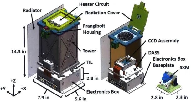
REXIS Instrument Description

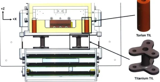
REXIS is comprised of two instruments, the larger Spectrometer and smaller Solar X-ray Monitor. The Spectrometer is mounted on the -Z deck of the spacecraft as shown in Figure 2-2a. The SXM is mounted on the -- X spacecraft gusset as shown in Figure 2-2b. During science operations, the -Z deck is asteroid facing and the X deck is sun facing. The Figure 2-3 shows the Spectrometer and SXM without MLI and with major components labeled. Starting at the bottom and working up the -Z axis, the Spectrometer has an electronics box that houses three electronic boards. The electronic boards communicate with the bus and regulate bus power for the Spectrometer and SXM. The PCBs also electrically interface with the detector assembly mount (DAM), which houses the four MIT Lincoln Laboratory built CCDs. Since the CCDs need to be cold in order to provide sufficient science data, the CCDs are thermally coupled to a cold radiator via a braided copper thermal strap. Two thermal isolation layers (TIL) thermally decouple the CCD assembly from the rest of the structure. The torlon TIL connects the DAM to the bottom panel of the tower

38

I

Heater Circuit

Radiator _{Radiation Cover}

Frangibolt Housing CCD Assembly 14.3 in ToweDASS Electronics Box TIL Baseplate _SXM +Z 2.8 in Electronics Box 7.9 in 5.6 in 2.8 in 2.3 in

Figure 2-3: REXIS Spectrometer and SXM shown with major components labeled

called the detector assembly support structure (DASS). The titanium TIL is bolted to the top of the electronics box and to the bottom of the DASS and structurally supports the entire tower. The tower houses the CCDs and supports the radiation cover assembly. To prevent radiation damage to the CCDs during the 2 year cruise out to Bennu, the Spectrometer has a radiation cover that closes off the CCDs to the space environment. When the spacecraft reaches Bennu, the cover will open via a one time use actuation mechanism that utilizes a frangibolt and spring hinge system. The frangibolt is mounted inside of the frangibolt housing and is kept warm via a heater circuit on top of the radiation cover. For more information on the design of the Spectrometer, see Carte [33]. For more information on the assembly and integration of the Spectrometer, see Bayley [34].

The SXM is a much smaller and less complex instrument. The SXM has one main bracket that structurally supports the backpack and SXM housing. The backpack and SXM housing both have small electronics boards mounted inside of them. The back-pack houses the backback-pack electronics board (SBB), and the SXM housing provides support for the SXM electronics board (SEB). The backpack electronics board con-ditions the voltage coming from the Spectrometer for the SEB. The SEB electrically

connects to and controls the SDD, which is cooled using an integrated thermo-electric

cooler (TEC) [351.

2.2.2

REXIS Mission Thermal Overview

After the launch of OSIRIS-REx, the satellite takes a two year cruise out to Bennu via an elliptical heliocentric orbit [241. During this cruise, REXIS is periodically powered on to perform self checkouts and internal calibrations. Since the orbit is eccentric, the thermal environmental loads, i.e. solar flux, seen during the cruise self checkouts and internal calibrations change over the course of the cruise period. The hot case occurs at the orbit's perihelion of 0.773 Astronomical Unit (AU) with a solar loading of -1.3 solar constants, and cold case at the orbit's aphelion of 1.39 AU or ~0.72 solar constants, as shown in Figure 2-4. Once OSIRIS-REx arrives at Bennu, the mission enters the Detailed Survey Phase in which the satellite maneuvers itself into a 1 km

terminator orbit around Bennu with the

+Z

deck fixed nadir to the asteroid [36]. The

Spectrometer is mounted on this nadir deck such that Bennu is down the boresight of the instrument. By this point, the Spectrometer has actuated the frangibolt and opened its cover to allow the CCDs to begin taking asteroid X-ray data. A mapping of estimated Bennu temperatures and solar reflectance (albedo) is incorporated into the REXIS thermal model. This additional heat load is neglected for the Detailed

Survey cold case to be conservative. For the hot case, although the presence of

Bennu does provide additional environmental loading to the Spectrometer, once the cover is opened, the heater circuits on the radiation cover and frangibolt housing are powered off, helping to offset this heat load and maintain the CCDs below their science temperature threshold. Table 2.2 summarizes the driving thermal cases for the REXIS instrument per mission phase. For more detailed information about the

3

IOutbound

0.9 h Cruise 0.7

/

I

Proximity Ops 12/2/2015 12/1/2016 12/1/2017 12/1/2018 12/1/2019 11/30/2020 11/30/2021 11/30/2022 11/30/2023

Figure 2-4: OSIRIS-REx Mission Solar Environment [6]

Table 2.2: REXIS driving thermal mission cases

Cruise Phase

Cruise, Hot Perihelion 0.773 2322.1 0 On Closed/On

Cruise, Cold Aphelion 1.387 700.1 0 Off Closed/On

Detailed Survey Phase

DS, Hot enPeilo,

135deg Brans erihelion, 0.897 1752 45 (+Z) Off Closed/On

Offpoint

DS, Hot Bennu Perihelion 0.897 1752 0 On Open/Off

Return Cruise

Table

OC

2.3: Spectrometer and SXM temperature requirements/QoIs per component in

Spectrometer Component Temperature Requirements

Component Operational Non-Operational

Electronics Boards -25 85 -35 85

Active PCB Components -40 110 -40 110

CCDs -120 -60 -120 60

Frangibolt/Cover Mechanism -20 80 -20 80

SXM Component Temperature Requirements

Component Operational Non-Operational

SDD Housing -40 100 -65 150

SEB -40 85 -55 85

SDD -100 -30 -

-2.2.3

REXIS Thermal Requirements

The Spectrometer thermal design is required to meet the four steady state compo-nent temperature criterion listed in Table 2.3. The temperature requirements for the electronics boards and CCDs differ between operational and survival modes of the Spectrometer. During operation, the PCB board temperatures shall not rise above 85"C. This requirement is derived from the temperature limits of the passive board mounted components. For the active board mounted components, each part is thermally analyzed to ensure the derated junction temperature limit is not violated.

As per NASA/TP-2003-212242, EEE-INST-002, active board mounted component

junction temperatures shall not exceed 110'C or 40'C below manufacturer published maximum junction temperature rating, whichever is lower. This derating ensures the reduction in stress applied to the part during normal operations in order to pro-long the expected life [371. Typically a cold operational analysis is not performed, as the hot operational case is far more stressing, because the component could en-ter an overheating operational failure mode. Likewise, the failure mechanism for the non-operational cases for the electronics boards becomes a thermostructural issue of potential coefficient of thermal expansion (CTE) mismatch. A thermoelastic analysis

was not completed for the Spectrometer PCBs. Instead, best practice engineering principles were used and testing verified the boards survival from -35 C to 60'C .

The Spectrometer CCDs also have different operational and non-operational ther-mal requirements. Operationally, the CCDs need to be less than -60'C to collect good science data [311. At -600C, there is sufficiently low dark current to meet performance requirements. The low limit on the CCDs for both operational and non-operational modes is set by the thermostructural limit. Engineering model (EM) CCDs were successfully tested down to -120*C and operated again. For the hot non-operational limit, the CCDs shall not exceed the 60'C tested limit. This tested limit is not a driving requirement as the CCDs stay well below this temperature for the duration

of the mission.

The temperature requirements of the frangibolt and cover mechanism are critical to ensure high confidence in cover deployment after the two year cold cruise period. The manufacturer published frangibolt temperature ratings are -50 C to +80*C for operation and down to as cold as -800C for survival. Although frangibolts have flown on and operated in past successful missions

1381,

this particular miniature model frangibolt has limited flight heritage, having only flown on the DICE cubesat

1391

and has not endured a long on orbit storage period before successfully firing. This lack of flight heritage and the temperature dependence actuation time findings in Carte

[401

present an increased risk to the contamination effects of the cover deployment due to possible prolonged firing time of the frangibolt. To reduce the uncertainty in frangibolt firing time, and increase the likelihood of the mission critical cover deployment, a requirement of long term frangibolt and cover mechanism temperature to be no colder than -20'C is imposed. The radiation cover heater circuit is designed to satisfy this requirement, but this heater circuit is limited by the bus to 10 W

average power usage during cruise.

The SXM thermal design is required to meet the three steady state component temperature criterion listed in Table 2.3. The SDD housing requirements are driven by the manufacturer's allowable temperature limits of the integrated SDD and TEC package. The SDD housing temperature is measured on the hot side of the TEC

4 +Z

2

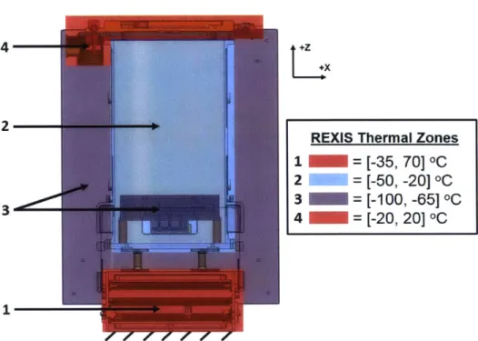
REXIS Thermal Zones

1 = [-35, 70] OC

2 = [-50, -20] OC

3 m =

[-100, -65] OC

I

4

[-20, 20]

OC

1

Figure 2-5: REXIS Spectrometer four thermal zones

where it interfaces with the SXM housing. The SEB requirements originate from the maximum and minimum allowable temperature ranges of the board mounted com-ponents. The SDD temperature requirements are derived from the limiting detector temperature at which science product degrades. If the SDD temperature require-ment is not met, the SXM will not produce usable data, but no component failure will occur. Since the first two SXM thermal requirements are based on component temperature limits, SXM catastrophic failure will occur if the SDD housing or SEB temperature requirements are violated.

2.3

Spectrometer Thermal Design Overview

The thermal design of the Spectrometer breaks up the instrument into four distinct thermal zones. Each zone is designed to operate over different temperature ranges to meet the REXIS thermal requirements/ QoIs listed in Table 2.3 and ensure mission success. Figure 2-5 shows the four thermal zones and their on orbit temperature ranges. Thermal zone 1 is a warm zone that is thermally coupled to the spacecraft