Application of damping in high-rise buildings

Application of Damping in High-rise Buildings

by

Jeremiah C. O'Neill Jr.

B.S. in Civil and Environmental Engineering Lafayette College

Submitted to the Department of Civil and Environmental Engineering in partial fulfillment of the requirements for the degree of

Master of Engineering in Civil and Environmental Engineering at the

Massachusetts Institute of Technology

M)

June 2006

0 2006 Jeremiah C. O'Neill Jr. All rights reserved

ASSACHUSETTS INSTnTfTE

OF TECHNOLOGY

JUN 0 7 2006

LIBRARIES

The author hereby grants to MIT permission to reproduce and to distribute publicly paper and electronic copies of this thesis document in whole or in part in any medium now known or

hereafter created

4

I I

Signature of Author...

Certified by ...

... ... ... .

Department of Civil and Environmental Engineering May 12, 2006

/

1/

4

Andrew J. Whittle Chairman, Departmental Committee for Graduate Students

BARKER

-4

Application of Damping in High-rise Buildings

Jeremiah C. O'Neill Jr.

Submitted to the Department of Civil and Environmental Engineering on May 12, 2006 in Partial Fulfillment of the

Requirements for the Degree of Master of Engineering in Civil and Environmental Engineering

ABSTRACT

The outrigger structural system has proven to be an efficient lateral stiffness system for high-rise buildings under static loadings. The purpose of this thesis is to research the incorporation of viscous dampers into the outrigger system to improve the dynamic performance. This study will be conducted on a typical high-rise structure in Boston, MA in attempt to find realistic results.

This thesis will utilize two analysis models for the study: a simplified single degree of freedom model and a more sophisticated computer model constructed with the structural analysis software, SAP2000. The models will be used to assess the effect that increasing damping or changing damper locations has on the dynamic performance of the structure. Furthermore, the constructability issues of each damping configuration will be identified and discussed.

Thesis Supervisor: Jerome J. Connor

ACKNOWLEDGEMENTS

First and foremost, I would like to thank my parents for giving me the opportunity to have the education I have had. I truly appreciate your dedication to providing your children with the best education possible.

I am also indebted to thank everyone who has helped with this thesis, particularly

Professor Connor. He has shared an exceptional amount of knowledge throughout the whole year, and without it, this thesis would have never been successful.

I also need to thank those that made this year an enjoyable experience and my life more

interesting then damping in high-rise buildings. So thank you Jill and all of you Meng kids.

TABLE OF CONTENTS

CH A PTER 1 IN TR O D U C TIO N ... 7

1.1 THESIS O BJECTIVE ... 7

1.2 OUTRIGGER STRUCTURE BASICS... 8

1.3 INTRODUCTION TO D AMPING ... 9

1.4 BUILDING D ESCRIPTION ... 1 1 CHAPTER 2 NUMERICAL ANALYSIS... 13

2.1 THE CONCEPT ... 13

2.2 N UMERICAL D ERIVATION ... 14

2.3 D IFFERENTIAL EQUATION SOLUTION ... 16

C H A PTER 3 STA TIC A N A LY SIS... 18

3.1 INTRODUCTION... 18

3.2 STATIC W IND LOADS AND DESIGN CRITERIA... 18

3.3 SIM PLE CANTILEVER SD OF ANALYSIS... 19

3.4 SIMPLE CANTILEVER SAP2000 STATIC ANALYSIS ... 21

3.5 O UTRIGGER SD O F STATIC ANALYSIS ... 22

CHAPTER 4 DYNAMIC ANALYSIS ... 25

4.1 INTRODUCTION... 25

4.2 BRIEF V ORTEX SHEDDING ANALYSIS ... 25

4.3 DYNAMIC WIND LOADS AND DESIGN CRITERIA ... 27

4.4 D ETERMINATION OF DAMPING COEFFICIENTS... 31

4.5 SD OF DYNAM IC ANALYSIS ... . . ... 33 4.5.1 Purpose... 33 4.5.2 Analysis Results ... 34 4.5.2.1 No damping ... 34 4.5.2.2 Equivalent damping of 10% ... 36 4.5.2.3 Effectiveness of damping... 39

4.6 SAP2000 DYNAMIC ANALYSIS OF CONFIGURATION A ... 40

4.6.1 Concept ... 40

4.6 2 Analysis Results... 41

4.6.2.1 N o damping ... 41

4.6.2.2 Equivalent damping of 10% ... 43

4.6.2.3 Equivalent damping of 20% ... 45

4.6.3 W hy is the equivalent damping so high?... 46

4.6.4 Construction considerations ... 47

4.7 SAP2000 DYNAMIC ANALYSIS OF CONFIGURATION B ... 48

4.7.1 Concept...48

4.7.2 Analysis Results ... 49

4.7.3 Constructability Concerns ... 52

4.8 SAP2000 DYNAMIC ANALYSIS OF CONFIGURATION C ... 53

4.8.1 Concepts... 53

4.8.3 Constructability Considerations... 56

CHAPTER 5 CONCLUSION... 58

CHAPTER 6 REFERENCES... 60

APPENDIX A MATLAB CODES... 61

A .1 ODE45 M A TLA B CODE ... 61

LIST OF FIGURES

Figure 1.1. Typical outrigger design (Hoenderkamp, 2003)... 9

Figure 1.2. Viscous damper (Taylor Devices, Inc.)... 10

Figure 1.3. Building D im ensions... 11

Figure 1.4. Cross-section of building with outrigger and damper layout ... 12

Figure 2.1. Continuous outrigger model ... 13

Figure 3.1. Bending rigidity versus outrigger column area ... 23

Figure 3.2. Optimum outrigger location (Smith, 1991)... 24

Figure 4.1. Transfer function for displacement (Connor, 2003)... 27

Figure 4.2. Transfer function for acceleration (Connor, 2003) ... 27

Figure 4.3. Forcing function for SAP2000 model ... 29

Figure 4.4. Forcing function for SDOF system ... 30

F igure 4.5. SD O F system ... 34

Figure 4.6. Top floor displacement with no damping and loading A ... 35

Figure 4.7. Top floor acceleration with no damping and loading A ... 36

Figure 4.8. Top floor displacement with 10% damping and loading A... 37

Figure 4.9. Top floor acceleration with 10% damping and loading A... 38

Figure 4.10. Dynamic model Configuration A ... 41

Figure 4.11. Top floor displacement with no damping and loading A ... 42

Figure 4.12. Top floor acceleration with no damping and loading A ... 43

Figure 4.13. Top floor displacement with 10% damping and loading A... 44

Figure 4.14. Top floor acceleration with 10% damping and loading A... 44

Figure 4.15. D amper force (kN) ... 47

Figure 4.16. Dynamic model Configuration B ... 49

Figure 4.17. Damper stroke under load B with no outrigger columns... 51

Figure 4.18. Damper stroke under load B with outrigger columns... 52

Figure 4.19. Dynamic model Configuration C... 54

Figure 4.20. Displacement at top and bottom of damper ... 55

Figure 4.21. Displacement at top and bottom of damper ... 56

LIST OF TABLES

Table 3.2. M odel param eters... 19

Table 4.1. Human perception levels of motion ... 31

Table 4.2. C values for corresponding equivalent damping... 33

Table 4.3. Top floor displacement and acceleration for steady state response... 36

Table 4.4. Top floor displacement and acceleration for 10% equivalent damping... 38

Table 4.5. Top floor displacement and acceleration for 10% equivalent damping... 45

Table 4.6. Top floor displacement and acceleration for 20% equivalent damping... 45

CHAPTER 1 INTRODUCTION

As cities continue to grow and land value continues to increase, buildings are

being built taller in an effort to maximize rentable space. The result is tall buildings on

small lots of land, which leads to higher building aspect ratios (height-to-width).

Furthermore, material advancements have yielded higher strength steels, but the modulus

of elasticity has remained constant. As materials advance in this way and building

become more slender the design shifts from strength based design to motion based

design. This means that the critical design is not the strength of the structural members

supporting the gravity loads, but the stiffness of the structure resisting the lateral loads.

When exposed to high winds, high-rise buildings may experience drifts on the magnitude

of meters, which causes concerns for serviceability and human comfort. For this reason,

one of the largest problems facing engineers today is drift control in high-rise structures.

This thesis will explore drift and acceleration control with viscous damping in an

outrigger structural system.

1.1 Thesis Objective

The outrigger structural system has proven to be an effective structural design, but

as in all slender buildings it can be susceptible to high drifts and consequently high

accelerations under dynamic loading. Passive damping has proven to be an efficient way

to reduce these unwanted effects. There are many forms of passive damping, but most

commonly damping systems come in the form of viscous damped braced frames or tuned

mass dampers. As will be explained in the following section, viscous dampers are most efficiently placed in a location where their differential velocity is maximized. Following

an outrigger where the displacement is magnified, but there is little to no research on this

application. This thesis will explore the effectiveness and feasibility of implementing a

viscous damping system in the outrigger structural system to help control building motion

and acceleration. This will be done by running analyses for a typical 40-story building in

the Boston area.

1.2 Outrigger Structure Basics

In order to meet building owner's demands for open space, building designers

have been locating lateral systems (braced steel frames, concrete shear walls, etc) in the

center of buildings where they can be disguised by mechanical shafts. This system

uncouples the core from the exterior columns, and uses the core as the only resistance for

the lateral forces. The outrigger design enables a building to activate its total width when

resisting lateral loads by coupling the core and the columns. The design consists of a

braced steel or reinforced concrete central core with cantilevered outriggers connecting to

exterior columns, as shown in Figure 1.1. When subjected to a lateral force the central

core is subjected to bending deformation which causes the outrigger to rotate. The

rotation of the outrigger is resisted by the exterior columns, which imparts a concentrated

bending moment that reduces the moment in the core and at the base. The addition of

outriggers provides no additional shear resistance, so the core must be designed to resist

the full shear force. The advantages of the outrigger structural systems as stated by The

Council on Tall Buildings and Urban Habitat are summarized below.

* _{"Core overturning moments and their associated induced deformation can be reduced} through the "reverse" moment applied to the core at each outrigger intersection.

" Significant reduction and possibly the complete elimination of uplift and net tension

forces throughout the columns and foundation system.

" The exterior column spacing is not driven by structural considerations and can easily

"

" For rectangular buildings, outriggers can engage the middle columns on the long faces of the building under the application of wind loads in the more critical direction." (Kowalczyk, 1995)

The main drawback of the outrigger system is the inference with interior space. Each outrigger is typically one or two stories deep, which makes the outrigger floors unrentable space. Most commonly, a mechanical floor is located at the outrigger level, but in tall buildings the most cost effective location for a mechanical floor is the basement so The Council on Tall Buildings and Urban Habitat proposed alternative ways of incorporating these systems.

* _{"Locating outriggers in the natural sloping lines of the building profile.}

" _{Incorporating multilevel single diagonal outriggers to minimize the member's} interference on any single level.

* _{Skewing and offsetting outriggers in order to mesh with the functional layout of the} floor." (Kowalczyk, 1995)

--

LfX-t

H

b Lc/) i c/h b

Figure 1.1. Typical outrigger design (Hoenderkamp, 2003)

1.3 Introduction to Damping

In structural building design, damping is the process by which a structure

----in this paper, operates by forc----ing a fluid through an orifice ----in turn creat----ing a resist----ing

force. Figure 1.2 shows an example of 1.5 million pound viscous damper from Taylor

Devices, Inc.

Figure 1.2. Viscous damper (Taylor Devices, Inc.)

The major benefit of viscous dampers is that they are dependent on the velocity of

the structure, which is completely out of phase from the maximum displacements (also

bending and shear stresses) in a building. Equation (1 1) defines the expression for the

damper force

Fdamper = c (1.1)

where c is the damping coefficient that describes a damper and i is the velocity.

Consider a building that is excited laterally by an earthquake. As the structure oscillates,

the columns reach their maximum stress when the displacement has reached its

maximum. At this point the structure instantaneously stops, meaning there is no velocity,

and therefore the force in the viscous dampers is zero. As the structure rebounds the

dampers reach a maximum output at the point of maximum velocity, which is also the

point of zero displacement and therefore a point of zero lateral stress in the columns. The

result is that viscous dampers can reduce the overall displacement and acceleration

1.4 Building Description

This thesis will analyze a 40 story outrigger structure in Boston, MA which is

shown in Figure 1.3. The floor height will be 3.5 meters giving a total building height of

140 meters. The building will be 30 meters wide, in order to achieve an aspect ratio of

about H/5. The construction method is assumed to be concrete slab/metal deck with steel

beams and columns, therefore the total weight of the building will consist of the weight

of concrete in slabs and the weight of structural steel. The mass was taken from

published data for an existing 40-story building in Boston, MA, with a total mass of 2

55,800 tons and a typical floor area of 2090 m2. (McNamara, 2000) After scaling the mass by the floor area being used in this thesis (900 in2_{) the mass of the building is taken}

m kg

as 24,000 tons, giving p = - =170, 000-. Lastly, Figure 1.4 shows a cross-section

H m

through the building showing the layout of outriggers and where dampers will be added.

There are eight outriggers cantilevering from the central core and connecting to different

configurations of columns and viscous dampers.

-- a5m 140mp

4

4

Outrigger

1W _w

II

Figure 1.4. Cross-section of building with outrigger and damper layout

I

Damper

---1W

CHAPTER 2 NUMERICAL ANALYSIS

2.1 The Concept

In order to explore the effect of dampers in the response of a structure with

outriggers, a single-degree of freedom (SDOF) model of the system was derived. The

structure was first simplified to a simple continuous cantilevered beam with infinitely

rigid outrigger arms that are attached to a spring and damper, as is shown in Figure 2.1.

The next step was to derive the equation of motion for the SDOF system, which was done

by transforming the continuous beam equations into a set of discrete equations.

U 14 -1 p, DB

Ji~

4

"4

d

II

W

14

II

PC

H

P C

I

I

2.2

Numerical Derivation

The derivation followed the procedure presented by Connor (2003) for the

fundamental mode response of a continuous beam. The derivation begins by expressing

the displacement and rotation in terms of generalized coordinates.

u = q(t)$(x) (2.1)

8 = q(t)$'(x) (2.2)

where $(x) is the fundamental mode shape and q is the modal amplitude parameter. The

analysis will consider the cantilever beam as a pure bending beam, meaning that there

will be no shear deformation. Therefore,

W (x X2(2.3) H

2x (2.4)

$'() = --2

The bending deformation X is related to q by

2 (2.5)

X =,,x =-7q

Using The Principle of Virtual Displacements (Bathe, 1995) the equilibrium

equation can be written in terms of q(t). The procedure begins by expressing the

displacement variables (u, P) in terms of generalized coordinates (q(t)). A virtual

displacement is defined as a displacement distribution created when the generalized

coordinate is excited by a small amount, 9q. This principle is based on the requirement

that the work done by the external loads during the virtual displacement must be equal to

the work done by the internal forces during the same virtual displacement. The

fMsxdx = Force * displacement + I Moment * rotation (26)

0

where M is the internal moment, Force is the externally applied loading and inertial

forces, and Moment is the externally applied moment by the outriggers. So this

expression becomes

H H(27

JMdXdx = fb5udx - (2.7)

0 0 h

b =

b

g

Assuming that both columns and dampers attached to the outrigger work in compression

and tension, the counter moment can be expressed as

-4e~hk 4e2

hc29

M = 2ekcou,,e sin, 1 + 2ecampere sin 4e2hkcolumn + damper q (2.9)

dapr h - H2 q H2

2 (2.10)

where b is a prescribed loading, mu is the inertial forces of the building, kcoim is the

axial stiffness of the columns attached to the outriggers, cda.per is the damping coefficient

of the dampers attached to the outriggers, and DB is the bending rigidity of the building

core. Although the bending rigidity of the building core would typically vary with the

height, this analysis assumes DB to be constant throughout the building height. Also, the

expression for the applied moment from the outriggers, M, assumes that the outriggers

solution. Using the definition of u given in equation (2.1), the virtual terms can be related to i5q. (5u =

8q

After substituting equations (2.11), (2.12), and (2.13) into equation (2.7) the equilibrium

equation becomes

H 4DB _{H 2x}

H4 _{q(qdx = Jb#6qdx - H}2 _Sq

0H0 h

(2.14)

and can be simplified to

H _4DB H4qdx f H 4 (2.15) H 12xM 0bodx -0~ 2

Following integration and substitution of terms the final equilibrium equation of motion

is expressed as pH . 8e2_h2_ca.,, q + damper 5 H4 (2.16) 8e2h2kumn +4DB

1=H

_j

₃

2.3 Differential equation solution

Equation (2.16) is expressed in the form of rniii + j + ku = jb which can be solved

using one of the internal differential equation solvers in MATLAB, such as ode45. The

ode45 function is used to solve initial value ordinary differential equations, using 4th and

main inputs: a function describing the differential equations, a vector indicating the time

of integration, and a vector defining the initial conditions of the system.

The ode45 function is setup to handle first-order equations and so the

second-order differential equation must be converted into an equivalent series of first-second-order

equations, as shown below

yj = q (2.17)

Y2= =

(2.18)

. .. p-ky1-cy2 P-kq-c4 (2.19)

m m

Next the time vector is created, which specifies the initial and final times that MATLAB

will integrate between. Lastly, the initial conditions of the system must be defined,

which in this case are q, =0 and 4, =0. Once these three inputs are defined the ode45

function can be run. The results give a vector of the time values, the displacement, and

the velocity. Knowing that the acceleration is the derivative of the velocity, a FOR loop

was created in MATLAB to calculate the slope between each point of the velocity vector.

CHAPTER 3 STATIC ANALYSIS

3.1 Introduction

Before moving to a complicated dynamic analysis, a static analysis was used to

verify that the simplified models were providing proper results. The static analysis is

used to calibrate the stiffness parameters of the models, and to investigate the effect of

certain parameters in the outrigger model.

3.2 Static Wind Loads and Design Criteria

The static wind loading was taken directly from the Massachusetts Building Code,

and is shown in Table 3.1. These wind loadings are based on a 145 km/hr wind speed,

which is a 100-year wind, and an exposure factor of B, which is for areas where % mile

upwind is continuous urban development, forest, or rolling terrain. Under the 100-year

wind the structure should be designed to have no serviceability problems, therefore the

H static deflection at the top of the structure was limited to .

500

Table 3.1. Wind Pressures

0-30 1005 31-45 1245 46-61 1436 62-76 1628 77-91 1772 92-122 1963 123-140 2202 Avera e 1607

3.3 Simple Cantilever SDOF Analysis

For the purpose of this thesis, as described earlier, the building being analyzed is

140 meters tall therefore H is set constant at 140. The analysis will also assume that there

are two braced frames and outriggers in each direction, as shown in Figure 1.4, therefore

each set will resist /2 the lateral forces. This assumption set the wind load (w) constant at

the average of the pressures in Table 3.1 (about 1600 Pa) times 2 the building width (15

meters), so w was taken as about 24,000 N/m. Lastly, the mass density of the building

was held constant as 170,000 kg/m as explained earlier. Since the SDOF system is

representative of one outrigger system (1/2 of the total system), the mass density used in

the analysis is /2 of the total. The values used in the analysis are summarized in Table 3.2.

Table 3.2. Model parameters

H (m) 140

p(kg/m) 85000

w (N/mA2) 24000

e (m) 15

The first step was to run the analysis as a simple cantilevered beam which is

representative of a braced frame core structure with no outriggers. This model can be

used as a control to compare the sensitivity of certain changes. The stiffness of this

structure is dependent on the provided bending rigidity, DB . To determine DB for this

system the maximum deflection constraint was applied to the top of the structure,

=H

q*=-= .28m . The expression for DB for a cantilever beam with a static uniform 500

DB-b[ H --X]2 (3.1)

DB

2X *

where b is the uniform loading, x is the distance up the building, and ;r * follows

equation (2.5) as

2 (3.2)

Since the SDOF solution is derived based on a constant DB , equation (3.1) is evaluated at

H

the point x = - = _{70m to average the typical rigidity distribution. This value of} DB is 2

about 2.OxlO" and is used for the bending rigidity of the full height. When the

MATLAB code is run using these values and ignoring the outriggers a maximum static

deflection of .38 meters is found and a period of 6 seconds. The deflection is higher than

predicted by the calculations above, and the period is higher than expected. The expected

period is .1 *N where N is the number of stories. Using this rule of thumb, this structure

should have a period of around 4 seconds. The cause of these inaccuracies is the

assumption of a constant DB The derivation is based on a specified mode shape, 0, as shown in equation (2.3). This mode shape can only be obtained by a bending rigidity that

varies with x. By implementing a constant bending rigidity, a new fundamental mode

shape is created.

Instead of solving for DB with an equation that assumes a varying DB, DB will

be solved for directly using equation (2.16). It is known that the static displacement is

bH (3.3)

Usac =k= _8e2_h2_kiun

+ 4

DB

Since in this case the outrigger is being ignored the equation is reduced to

gH4 (3.4)

U = 12DB

H

Again specifying q* = -=.28m, DB is determined as 2.75x1012_{. When entering this}

500

value into MATLAB, Umax is found to be .28 meters, as expected, and the period is calculated as 4.8 seconds, which is closer to the expected value. These results were

considered acceptable for static response, so the next step was to build a model in

SAP2000 for further verification.

3.4 Simple Cantilever SAP2000 Static Analysis

In order to obtain more accurate results, a model was constructed in the structural

analysis program SAP2000. The braced core was represented as a single cantilevered

element with properties representing that of a braced frame building. The mass, loading,

and height are those specified in Table 3.2. The stiffness was determined by using the

conventional equation for deflection at the top of a cantilever beam subjected to a

uniform load and limiting deflection as shown below.

Umax =.28m (3.5)

wH4 (3.6)

Umax

8EI

Solving equations (3.5) and (3.6) for EI, the bending rigidity is found to be

DB = 4. xl 012 . Upon running the analysis it is found that umax =.28m as expected, and

the fundamental mode is found to have a period of 5.0 seconds, which is acceptable.

model. This inconsistency is again the cause of the mode shape assumption as described

above. The fundamental period of both models is comparable, about 5 seconds.

3.5 Outrigger SDOF Static Analysis

In the static case two parameters, the column stiffness (k,,u.) and the outrigger

height (h), will have an effect on the stiffness of the SDOF system. The length of the

cantilevering outrigger, e, would also effect the stiffness, but in this case the building

dimensions are fixed at 30 meters making e an irrelevant parameter. The first portion of

this section will explore the sensitivity of the aforementioned parameters.

To understand the effect of changing kcoiu.n a comparison can be made between

how an increase in kcou.,n decreases the necessary DB . The column is treated as a simple

axial member with stiffness, kc,,u.n, expressed as

kcoiumn - AE (3.7)

h

For the static case, DB can be expressed as a function of the column area

D H3 bH 8e2h2AEj (3.8)

B 41q*

hH' _{_}

In this equation H, e, q*, and b were defined earlier. E is the elastic modulus of steel,

210x10 -- , and h will vary from points of the full height (35m, 70m, 105m, and m

140m).

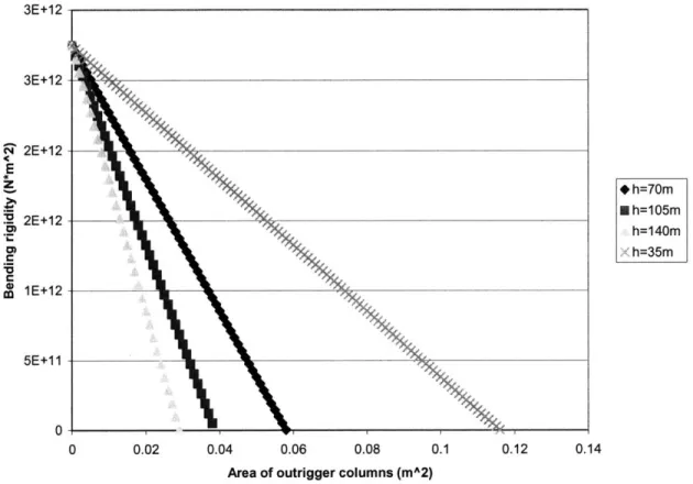
Figure 3.1 shows the linear relationship between bending rigidity and outrigger

column area. As expected, when the column area increases the necessary bending

point is reached where zero bending rigidity is required. But by comparing the column

stiffness needed for each plot to reach zero bending rigidity it is clear that there is an

inversely proportional relationship between outrigger height and column stiffness. That

is, as the height of the outrigger decreases the column stiffness must increase to obtain an

equal bending rigidity.

zC E) 0 3E+12 3E+12 2E+12 2E+12 1E+12 5E+11 * h=70m M h=105m h=140m X h=35m 0 0 0.02 4 0.06 0.08

Area of outrigger columns (mA2)

Figure 3.1. Bending rigidity versus outrigger column area

These results are approximate as many simplifications have been made in this

SDOF model. First, the continuous model shown in Figure 2.1 is an infinite degree of

freedom system which is converted to a SDOF by lumping all mass, stiffness, and

loading resulting in the model shown in Figure 4.5. This model can give a good first .1 0.12 0.14

analysis above showed that if enough stiffness is provided in the columns with the

outrigger at % the building height, zero bending rigidity is required. This analysis fails to

realize that when the outrigger is at 2 the building height there is % of the building above

the outrigger acting as a cantilever, where bending rigidity must be provided. Also, as

mentioned earlier, the SDOF model assumed a pure bending beam meaning that there

would be no shear deformation. One must realize that this analysis has been focusing

solely on bending rigidity, but there must be sufficient shear rigidity to resist the shear in

the building, because an outrigger system will not provide any.

Smith (1991) has derived the equations that define an outrigger under uniform

static loads. Using these equations Figure 3.2 was derived to show the optimum location

of a building with one outrigger. In the figure co represents a ratio that characterizes the

flexibility of the outrigger; it increases as the flexibility increases. For the case of this

thesis, the assumption will remain that the outrigger is infinitely rigid, therefore o can be

assumed as zero. This assumption creates an optimal outrigger location of about 1/2 the

total building height, which will be used from this point forward.

0.1-02

0.

o 50 0. 0.4 0.6 0.8 1.O

Value of W

CHAPTER 4 DYNAMIC ANALYSIS

4.1 Introduction

The next step is to look at the dynamic response of the SDOF system. Due to the

high period of the structure an earthquake will have little effect on the structure because it

will not excite it at resonance. A more critical loading is a periodic wind loading that

could potentially excite the fundamental mode of the structure. In fact most design codes

state that any building with an aspect ratio greater than 4 or 5 will behave dynamically

when subjected to wind (Smith, 1991), which validates this dynamic analysis. This

loading could occur in two forms: vortex shedding or fluctuating wind gusts. The main

dynamic analysis will focus on fluctuating wind gusts, but the next section is a brief

analysis of the effects of vortex shedding.

4.2 Brief Vortex Shedding Analysis

The phenomenon of vortex shedding creates a response that is perpendicular to

the wind loading, a cross-wind response. This type of response is difficult to quantify

due to the sensitivity to building geometry, building density, turbulence factors, and

upwind buildings effects. (Smith, 1991) If the proper conditions exist a specific wind

speed can create building oscillation at the fundamental frequency. This effect can be

estimated by calculating the vortex shedding frequency as expressed below.

SrV (4.1)

f=

D

where ST is the Strouhal number which is taken as .2, V is the wind velocity, and D is

case that the building is excited at resonance. Evaluating equation (4.1) gives a critical

velocity of 108 km/hr, which is below the 100 year wind of 145 km/h, meaning this

building is vulnerable to vortex shedding at its natural period. Damping can help control

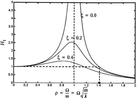
the problem, but nevertheless displacement and acceleration will be magnified. Figure

4.1 and Figure 4.2 show the transfer functions for displacement and acceleration, H, and

H2. These transfer functions make it possible to find the dynamic response as taken from

Connor (2003)

Udymic = Hjustatic (4.2)

p

dynamic 2

Connor (2003) also states that the maximum values for H, and H2 when damping values are small are

H

Im

These maximum values occur at resonance meaning that when vortex shedding occurs at

the buildings natural frequency the transfer function will equal equation (4.4). If an

assumed value of =.1 is used, the amplification of the static response will be 5.

Considering that damping of structures rarely exceeds 10% this can be considered the

best case scenario. The other option is to change the aerodynamics of the building so that

I:

Figure 4.1. Transfer function for displacement (Connor, 2003)

5 4.5-0.0 4 3.5 -2 0 1.5----- ---- ---.---.-0.s5.7 0 0.2 0.4 0.6 0.8 1 1.2 1.4 1.6 1.8

Figure 4.2. Transfer function for acceleration (Connor, 2003)

4.3 Dynamic Wind Loads and Design Criteria

The second type of dynamic wind is periodic gusts. Wind is a turbulent flow that

is characterized by random fluctuations in velocity and pressure. Standard static wind

1.8 2

2

V

the wind speeds are looked at as a function, certain periodic gusts within the wide

spectrum of wind may find resonance with natural frequency of the building, and

although the total force caused by that particular gust frequency would be much less than

the static design load for the building, dangerous oscillations may be set up. In order to

get a true response of the structure a detailed wind prediction would be conducted, which

would assess the local wind climate and surrounding topography to create a wind velocity

spectrum. This spectrum tends to be random in amplitude and is spread over a wide

variety of frequencies. Although the spectrum tends to be random, if any bands of the

spectrum fall near the natural frequency of the building a resonant response can occur.

(Smith, 1991) Typically, the structure would be subjected to a wind tunnel test or a wind

velocity spectrum to determine if there was a dynamic response, but since these are not

available for this thesis a forcing function will be created.

The goal in designing the forcing function was to make a somewhat realistic

representation of wind loading. Due to the sporadic nature of wind, it would be

unrealistic to subject the structure to a series of strong wind gusts with the natural period

of the structure. Instead, the function was created to represent two successive wind gusts

as impulse loads that had periods close to the natural period of the structure, which is

1 2 3 4 5 Time (s)

6 7 8 9

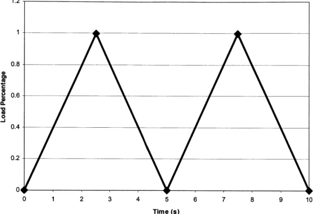
Figure 4.3. Forcing function for SAP2000 model

The function runs linearly from zero to the peak amplitude in 2.5 seconds and

then returns to zero in another 2.5 seconds, leaving a total duration of 5 seconds; this is

repeated twice. This function was easily input in the SAP2000 models, but the function

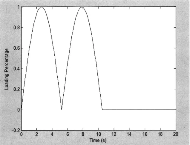
was idealized as sinusoidal function for simplicity in the SDOF analysis. The function

was taken as a piece-wise function as described below and shown in Figure 4.4

F = sin(nt) F = - sin(Qt) - <t --(4.5) (4.6) (4.7) F=O 1 2) 0 _j 0 0 0 0 10 . .8 .6 .4 .2 04 0

Figure 4.4. Forcing function for SDOF system

The analysis will focus on two amplitudes: the 100-year wind (loading A hereon)

and /2 the 100-year wind (loading B hereon). The 100-year wind applied in a dynamic

fashion can be considered as an extreme loading, in fact it may be unreasonably high.

Considering the return period of this amplitude is 100 years, the chance of the 100-year

wind occurring as two periodic gusts has an even smaller likelihood. For this reason, the

2 100-year amplitude, which is a more realistic loading, will also be applied.

The design criteria for the dynamic wind loading will not be as severe as the static

wind loading due to probabilistic nature of the event. Instead of limiting maximum

H H

displacements to H , the criteria will be lowered to . This criterion will ensure that

there is no damage to the non-structural elements during the dynamic loading. Secondly,

under the dynamic effects the designer must consider human perception of movement.

The topic of human comfort has been widely studied, but still there are no accepted

standard. (Smith, 1991) Table 3.1 shows how humans will perceive different levels of

acceleration where the critical design zone is defined as .1 to .25 m/s2_{. This is the range}

that humans begin to perceive the accelerations, but the criteria cannot simply be to limit

maximum accelerations to .2 m/s2_{. The reason is that it can be acceptable if a structure}

has accelerations greater than the acceleration criteria on occasion, because it will only

cause momentary discomfort for the occupants. Instead, the problem is when

accelerations continuously exceed the criteria. For this reason the acceleration design

criteria will use engineering judgment to determine the critical acceleration, and that must

be limited to .2 m/s2 _{during the dynamic response.}

Table 4.1. Human perception levels of motion

Critical Zone

U.Ub Humans cannot perceive motion

0.05-0.10 _{Sensitive people can perceive motion; hanging objects}

may move slightly

0.1-0.25 _{Majority of people will perceive motion; long-term}

exposure may produce motion sickness

0.25-0.4 Desk work becomes difficult of almost impossible

0.4-0.5 People strongly perceive motion; difficult to walk

0.5-0.6 Most people cannot tolerate motion and are unable to

walk naturally

0.6-0.7 People cannot walk or tolerate motion

>0.85 _{Objects may begin to fall and people may be injured}

4.4 Determination of Damping Coefficients

Typically damping of a structure is defined by an equivalent damping ratio, 4,

can be greatly increased. For the outrigger system the damping parameter 0 is taken

from the derivation in equation (2.16) as

8e2

h2cdamper (4.8)

H4

It is also known that a system governed by tn +

4

j (4.9)

By equating equations (4.8) and (4.9) the damping coefficient for the dampers can be

expressed as a function of ,.

2VZ H4 (4.10)

Cdamper 8e2h2

where k and rn are taken from equation (2.16) as

~ 8e2_h2_{kcl, 4DB (4.11)}

k = coun+ B

H4 _H3

- pH (4.12)

5

Using expression (4.10) damping coefficient values were calculated for given damping

ratios. The damping coefficients were inputted for the dampers in the analysis program

to obtain a damped dynamic response. In order to verify the calculations, a logarithmic

decrement analysis was used to determine the damping ratio from the dynamic response.

The method relates the change of amplitude between two successive peaks of a free

vibration damped response to the equivalent damping ratio as shown below

I In u (4.13)

where

j

needed to achieve several equivalent damping ratios for a system with a fundamental

period of 5 seconds.

Table 4.2. C values for corresponding equivalent damping

c (kN*s/m) 0.02 5183 0.04 10366 0.06 15549 0.08 20732 0.1 25916 0.2 51831

4.5 SDOF Dynamic Analysis

4.5.1 Purpose

The SDOF model, as shown in Figure 4.5, will be evaluated using the derived

equation of motion in equation (2.16) to determine the displacements and accelerations of

the system under dynamic loading. The results will be used to provide a general

understanding of the effectiveness of dampers in an outrigger structure and to verify the

k

k

C

C

Figure 4.5. SDOF system

4.5.2 Analysis Results

4.5.2.1 No damping

The first analysis was run with zero damping to note the response and use the

results as a comparison point for further tests. Figure 4.6 shows the displacement at the

top of the structure due to the dynamic loading of the 100-year wind. Since there is no

damping in the structure the conditions present at the end of the forcing function (t=10

seconds) create a typical response of a free vibration system with no damping. This

produces a maximum displacement of .79 meters which is about 60% greater than the

H

displacement criteria of -. Figure 4.7 shows the acceleration at the top floor with

300

respect to time. The same free vibration behavior is noted with a maximum acceleration

of 1.11 m/s2 that occurs at t= 8 seconds, which is 5.5 times the allowable acceleration of .2 m/s2. Since this is a steady-state response the maximum acceleration occurs

100-year wind the plots retain the same shape but the amplitudes are reduced by 50%. This

gives a maximum displacement under loading B of .4, which already meets the criteria.

Again this analysis shows the undamped dynamic response of the system, which

makes it evident that the dynamic response needs to be reduced in order to meet the set

acceleration criteria. These results are summarized in Table 4.3 and will be used as a

control to measure the effects of adding damping to the system.

Figure 4.7. Top floor acceleration with no damping and loading A

Table 4.3. Top floor displacement and acceleration for steady state response

A-

B-4=0 1 00-year 1/2 1 00-year

wind wind

amplitude amplitude Criteria

0.79 0.395 0.467

1.11 .55 0.2

4.5.2.2 Equivalent damping of 10%

Now that the undamped response is understood, the analyses will proceed with damping to note the reductions of displacements and accelerations. Figure 4.8 and Figure 4.9 show the SDOF response to the dynamic function with amplitude of the 100-year wind with a 10% equivalent damping ratio, and Table 4.3 summarizes the results.

It should be noted that, during the 10 seconds of the forcing function, the building has a greater response in the direction of the loading, whereas the undamped model had equal response in both directions. The addition of damping allows dissipation of strain

energy during the building's rebound from the force, which causes the unsymmetrical

response plot. Once the forcing function ends, the system begins free vibration about the

x-axis.

Figure 4.9. Top floor acceleration with 10% damping and loading A

Table 4.4. Top floor displacement and acceleration for 10% equivalent damping

A-

B-1 00-year 1/2 1 00-year

wind wind

amplitude amplitude Criteria

The addition of dampers has reduced the displacement by about 30% so that the

H

system easily meets the displacement criteria of under loading B. The results give a

300

maximum acceleration of .315 m/s2 and a critical acceleration of about .29 m/s2 for

loading B, meaning that the accelerations are still 30% higher then the set criteria.

The dampers have proven to greatly reduce the dynamic effects, but in order to

meet the acceleration criteria the equivalent damping must be increased further. The

and gaining a basic understanding of the damped outrigger dynamic performance. As the

SAP2000 model is expected to yield the most accurate results, a more comprehensive

analysis will be carried out.

4.5.2.3 Effectiveness of damping

This section will briefly use the SDOF model to compare the effectiveness of

dampers as a means for controlling dynamic response versus the other possible

alternatives: mass and stiffness.

By setting the equivalent damping to zero, the SDOF equations of motion can be

used to find what change in mass and stiffness are needed to obtain the same response as

the 15% damped system. The analysis yields that either mass needs to be increased by a

factor of 2.4 or the stiffness increase by 55% to achieve the same results. Increasing the

mass has the cost of the actual material added for the mass, but also the added structural

steel needed to carry the heavier loads to the foundations. Increasing the stiffness by

55% is a more difficult to put into perspective, but with this stiffness the static H

displacement becomes .1 m which corresponds to a displacement criteria of H . This 1400 criterion is about three times more than the static displacement criteria stated. To truly

compare the three alternatives a cost estimate would need to be conducted, but by using

the reasoning stated above it appears that the eight dampers providing 15% equivalent

4.6 SAP2000 Dynamic Analysis of Configuration A

4.6.1 Concept

As described earlier, an outrigger is traditionally used to provide a

counter-moment to the central core, which in turn reduces the necessary bending rigidity. This

concept utilizes the moment arm to provide a large resisting force with a comparatively

small amount of material. Configuration A will look at the dynamic effect of installing a

damper in parallel with the stiffness element at the end of the outrigger, which is the

same model that was generalized in the SDOF system. The damper is connected to the

end of the outrigger and the ground, whereas in typical applications a damper is

connected to two adjacent floors. In the typical setup, the damper only experiences the

differential movement between the two floors. In this application, since the ground is a

fixed point the differential movement in the damper will be the full magnitude of the

vertical movement of the outrigger. Remembering that the damping force is proportional

to the velocity, this setup should be highly efficient for a damper.

Figure 4.10 is representative of the model created in the structural analysis

program SAP2000. The system was subjected to the wind loading function shown in

Figure 4.3 with amplitudes of both the 100-year wind and V the 100-year wind. The

axial members connected to the outrigger were assigned an area of 171 cm2_{, the bending}

rigidity of the central core was calibrated to meet the 100 year wind static loading

p,

DB

k

k

C

C

Figure 4.10. Dynamic model Configuration A

4.6.2 Analysis Results 4.6.2.1 No damping

The first analysis was run with the zero damping to note the response and use it as

a comparison for further test. Figure 4.11 shows the displacement at the top of the

structure due to the dynamic loading of the 100-year wind. Similar to the results found in

the SDOF system, the system has forced vibrations during the 10 seconds of the forcing

function followed by constant free vibration. Again, almost matching the SDOF system,

there is a maximum displacement of .78 m as compared to the SDOF maximum

time. The same free vibration behavior is noted with a maximum acceleration of 1.25

M/s2, which is about a 10% difference from the maximum acceleration found in the

SDOF model. As stated earlier, for an amplitude of 2 the 100-year wind the plots would

retain the same shape but the amplitudes would be cut in !/. Continuing the comparison

of the SAP2000 plots and the SDOF system plots, they appear to be very close in shape

and amplitude. The main difference is the noise in the acceleration plot of the SAP2000

model. In comparison to the SDOF acceleration plot, Figure 4.7, the SAP2000 response

is not as smooth as it has micro-vibrations. This problem is the cause of the SAP2000, an

infinite degree of freedom system, being mildly excited at a higher mode causing small

vibrations along the fundamental response. The SDOF model, by definition, only has one

mode and therefore cannot experience effects from higher frequencies. Overall, the

results are close enough to verify that both models are creating accurate outputs.

(9.71 A.50) _0~ 5.K8. 12 1

Figure 4.12. Top floor acceleration with no damping and loading A

4.6.2.2 Equivalent damping of 10%

Following the procedure of the SDOF analysis, the SAP2000 model was next analyzed with 10% equivalent damping. Figure 4.13 and Figure 4.14 show the system response to the dynamic function with amplitude of the 100 year wind with a 10% equivalent damping ratio (c=25916 kN*s/m), and Table 4.3 summarizes the results.

4 W Legend-

-400,

0(18.855.784E-01 Fu-_ 4.03. T rdOK

Figure 4.13. Top floor displacement with 10% damping and loading A

18.17, 7.177E-01J

OK

Table 4.5. Top floor displacement and acceleration for 10% equivalent damping

Again, the plots from the SDOF model and the SAP2000 model are almost

identical in shape and magnitude. Since both the undamped and now damped responses

have matched in both models, the conclusion can be drawn that both models are accurate.

As was already stated in the SDOF section, the dampers have provided a large reduction

in displacements and accelerations, but the accelerations are still 35% greater than the

allowable, so the damping must be increased.

4.6.2.3 Equivalent damping of 20%

Table 4.6 shows the displacements and accelerations for loadings A and B with

20% equivalent damping. This damping value lowers the displacement in both loadings

well below the specified criteria, and gives a maximum acceleration value that is just

below the specified criteria when subjected to loading B. This means that if the 'A

100-year loading was the design dynamic loading, this structure would need 20% equivalent

damping to meet the design criteria.

4.6.3 Why is the equivalent damping so high?

Although 20% equivalent damping is typically considered as uneconomically

high, this system obtains this equivalent damping rather easily due to the amplification of

velocities and displacements. Looking back at Equation (1.1), the damper resisting force

is the product of velocity and the damper coefficient, c. Therefore, there are two ways to

increase the equivalent damping of a system, that is, the more traditional method,

increase the damping coefficient of the damper or increase the velocities.

According to Taylor Devices Inc., "In theory, there is no limit to the c value in

practice, you are limited by how small you can machine the actual orifice." That said,

although there is no theoretical minimum, at a point there is an economical minimum

where the manufacturing of a single damper will be more expensive then just increasing

stiffness. Also, if a designer is trying to achieve a certain damping force at a low velocity

Equation (1.1) would suggest an increase c, but, according to Taylor Devices, Inc., at low

velocities there may not be enough energy flux to overpower the structures inherent

structural damping. It is clear that increasing the damping coefficient may not always be

the most efficient answer to dynamic problems.

On the other hand the outrigger system effectively magnifies the rotations of the

core to a point where a high damping force can be achieved with lower damping

coefficients. This results in a higher equivalent damping ratio at a lower damping

coefficient and therefore a lower cost. Figure 4.15 shows the force in the damper during

the excitation of the 100-year wind, which records a maximum force of about 2113 kN

(about 475 kips). Taylor Devices, Inc. states that they manufacture viscous dampers with

force capacities ranging from 2 kips to 2,000 kips, which places this damper force on the

creating a damping ratio of 20% is not unreasonable, in fact the damping ratio could be

increased.

L n Legend E

Figure 4.15. Damper force (kN)

4.6.4 Construction considerations

The above results have proven that adding dampers to the outrigger system is an

efficient way to reduce the dynamic effects, but the constructability of such a system

must be looked at. The system analyzed above utilizes a damper that connects between

the ground and the outrigger at mid-height (70 m). Although the damper will not

physically be 70 m in length, it is critical that the damper is connected directly to the

ground to maximize the displacements and velocity. If the damper were connected to a

floor below the outrigger the damper would only be subjected to the differential

This setup would have the damper connected directly to the outrigger and an

element (possibly a column) that connected the damper to the foundation. The element

that connects the damper to the ground must span close to 70 meters, and will be

subjected to large tension and compression loads. The member must be designed to have

minimal axial deformation because the internal axial deformations will decrease the

displacement and velocity experienced by the damper. A column would be the best

choice, but should be braced at each floor to prevent buckling. If the compression forces

become a design problem the system can be altered to only activate the tension side of the

building. This would enable cables to be used as the connecting element. If cables were

used, only the damper subjected to tension in the cable would work at any given time,

therefore the damper would need to be engineered with double the damping coefficient to

achieve the same equivalent damping.

4.7 SAP2000 Dynamic Analysis of Configuration B

4.7.1 Concept

As stated earlier, a damper is most effective in a location that maximizes the

stroke or differential displacement between the two connection points. Configuration A

applied the damper in parallel with the axial member, which in effect limited the differential displacement of the damper to the axial strain in the axial member. In an

attempt to increase the displacement at the damper the axial column was removed from

the model, as can be seen in Figure 4.16. By doing this the central core must be restored

to the full bending rigidity for a cantilever beam, DB = 4.1X1012_{, to meet the static loading}

p,

U-C

C

Figure 4.16. Dynamic model Configuration B

4.7.2 Analysis Results

Figure 4.17 and Figure 4.18 show the displacement of the damper in

Configuration A and B when subjected to the / 100-year dynamic wind loading. When

compared it is clear that Configuration B has increased the displacement in the damper by

JME

Figure 4.17. Damper stroke under load B with no outrigger

Legend (29.90,-1.521E-02) OK columns F Legend --OK

Figure 4.18. Damper stroke under load B with outrigger columns

Table 4.7The increased damper stroke further decreases the displacements and

accelerations as shown in Table 4.7. The new configuration led to a decrease in top-floor

configuration yields an improved damper performance, but this may not be economical. A cost analysis would need to be conducted comparing the cost associated with

increasing the bending rigidity of the core in Configuration B versus the cost associated

with increasing the damping coefficient in Configuration A to achieve the results of

Configuration B.

TIME

-Legend--I

OK

-3 -Legend

2.-4O.4

0(26.25-1.978E-02

0, 15. 0OK

Figure 4.18. Damper stroke under load B with outrigger columns

Table 4.7. Comparison of displacement and acceleration of Configurations A and B

c=5,1831 kN-s/m Configuration Configuration

A B Criteria

0.22 0.18 0.2

4.7.3 Constructability Concerns

Again, the feasibility of implementing a structural system must be looked at realistically no matter how favorable the theoretical results are. The main concern with this system is the differential movement between the outrigger and the floor at that level. Although this analysis has assumed the outrigger to be infinitely rigid, the reality of the problem is that the outrigger will deflect up and down. This movement will be too large for any gravity structural system to be connected to the outrigger. The implementation of this system must allow for the outrigger to move independently of the surrounding

structural systems. This could be achieved using a form of an expansion joint between

the two structural systems, but further research should be conducted.

4.8 SAP2000 Dynamic Analysis of Configuration C

4.8.1 Concepts

Configuration C is shown in Figure 4.19. This alteration is a traditional outrigger

structure with dampers running from the middle outriggers to another set of outriggers at

the top of the building. This configuration allows the stiffness elements to be included in

the bottom half of the building giving the benefit of a reduction in the central core

bending stiffness. The theory is that the dampers will be subjected to the differential

movement between the top floor and the middle floor which should be similar to the

differential movement in Configuration B, while at the same time the central core

stiffness is reduced. The stiffness elements were input identical to Configuration A; the

central core bending rigidity was DB =3.08x1012 _{and the axial members had an area of}