Automatic design tool for robust radio frequency decoupling matrices in magnetic resonance imaging

Automatic Design Tool for Robust Radio Frequency

Decoupling Matrices in Magnetic Resonance Imaging

by

Zohaib Mahmood

Cla

C)w

Submitted to the School of Engineering

in partial fulfillment of the requirements for the degree of

0c

Cn 0

Master of Science in Computation for Design and Optimization

&

at the

MASSACHUSETTS INSTITUTE OF TECHNOLOGY

February 2015

@

Massachusetts Institute of Technology 2015. All rights reserved.

Signature redacted

Author ...

Signature redacted

School of Engineering

January 9, 2015

C ertified by ...

...

Luca Daniel

Emanuel E. Landsman Associate Professor of Electrical Engineering

and Computer Science

Thesis Supervisor

Signature redacted

A ccepted by ...

...

. o as G. Hadjiconstantinou

Automatic Design Tool for Robust Radio Frequency

Decoupling Matrices in Magnetic Resonance Imaging

by

Zohaib Mahmood

Submitted to the School of Engineering on January 9, 2015, in partial fulfillment of the

requirements for the degree of

Master of Science in Computation for Design and Optimization

Abstract

In this thesis we study the design of robust decoupling matrices for coupled transmit radio frequency arrays used in magnetic resonance imaging (MRI). In a coupled par-allel transmit array, because of the coupling itself, the power delivered to a channel is typically partially re-distributed to other channels. This power must then be dissi-pated in circulators resulting into a significant reduction in the power efficiency of the overall system. In this thesis, we propose an automated approach to design a robust decoupling matrix interfaced between the RF amplifiers and the coils. The decoupling matrix is optimized to ensure all forward power is delivered to the load. The decou-pling condition dictates that the admittance matrix seen by power amplifiers with 50 Ohms output impedance is a diagonal matrix with matching 1 (or 0.02 Siemens) at the diagonal. Our tool computes the values of the decoupling matrix via a non linear optimization and generate a physical realization using reactive elements such as inductors and capacitors. The methods presented in this thesis scale to any arbi-trary number of channels and can be readily applied to other coupled systems such as antenna arrays. Furthermore our tool computes parameterized dynamical models and performs sensitivity analysis with respect to patient head-size and head-position for MRI coils.

Thesis Supervisor: Luca Daniel

Title: Emanuel E. Landsman Associate Professor of Electrical Engineering and Com-puter Science

Acknowledgments

I would like to thank Prof. Luca Daniel for his guidance and mentorship. I am

grateful to Professor Jacob White, Professor Elfar Adalsteinsson, Professor Lawrence L Wald and Dr. Mikhail Kozlov for excellent technical discussions. I would like to thank Kate Nelson at the CDO office for her support. Last but not the least, I am thankful to my friends, colleagues and my family.

Contents

1 Introduction 11

2 Background 15

2.1 Decoupling Condition... . 15

2.2 Properties of a Decoupling Matrix . . . . 16

2.2.1 Lossless Components . . . . 17

2.2.2 R eciprocal . . . . 17

3 Design of a Decoupling Matrix 19 3.1 M ethod . . . . 19

3.2 The Optimization Problem . . . . 19

3.3 Enforcing Sparsity . . . . 20 3.4 Enforcing Structure . . . . 21 3.5 Robustness Criterion . . . . 23 3.6 Sensitivity Analysis . . . . 25 4 Results 27 4.1 A 16-Channel Array . . . . 27 4.2 A 4-Channel Array . . . . 31 4.3 D iscussion . . . . 32

5 MRI Sensitivity Analysis 37 5.1 P urpose . . . . 37

5.3 Results and discussion . . . . 40

List of Figures

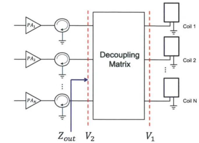
1-1 Block diagram of a parallel transmission RF array. A decoupling ma-trix is connected between the power amplifiers and the array. V and

V2 are the voltage vectors at the array and the power amplifiers

re-spectively. ZOUT is the impedance matrix of the load seen by power amplifiers. Perfect decoupling and matching is obtained when ZOUT is a diagonal matrix with diagonal entries equal to the output impedance of the power amplifiers. . . . . 13

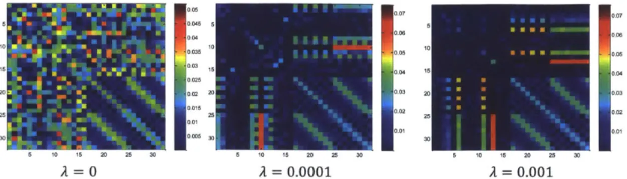
3-1 Sparse decoupling matrices with similar performance for the same prob-lem computed with different values of A. Blue pixel indicates a zero. . 21

3-2 Performance with a structured decoupling matrix . . . . 22

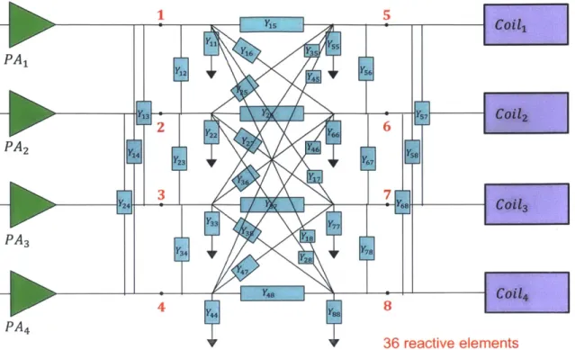
3-3 Schematic of a fully dense decoupling matrix. The elements YKj

indi-cate a reactive element connected between the nodes i and

j.

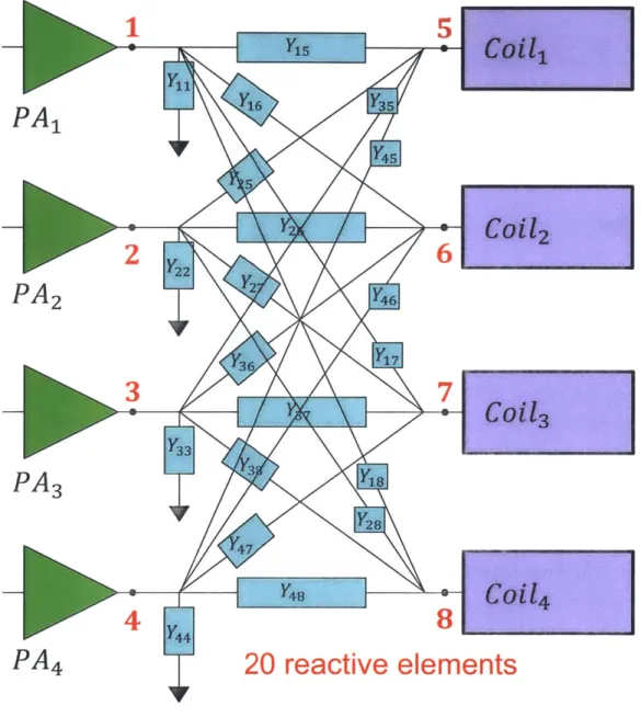
. . . . 23

3-4 Schematic of a structured decoupling matrix. The elements Yjj indi-cate a reactive element connected between the nodes i and

j.

Note that the number of reactive elements decrease from 36 to 20. . . . . 24

4-1 EM simulation of a pTx coil with 16 channels distributed in 2 rows. 28

4-2 Convergence curves . . . . 28

4-3 Magnitude of one of the possible decoupling matrices . . . . 29

4-4 Coupling coefficient matrix WITHOUT the decoupling network . . . 29

4-5 Coupling coefficient matrix WITH the decoupling network . . . . 30

4-6 Local SAR vs. fidelity L- curves (slice-selective RF-shimming) . . . . 30

4-8 Picture of the coupled 4-channel 7T parallel transmit head array to be decoupled. . . . . 32

4-9 S-parameters of the array without a decoupling matrix. Sjj indicates the reflection at port i, while Sij indicates the coupling between ports iand j. ... ... 33

4-10 Schematic of the decoupling matrix. The elements Yj indicate a reac-tive element connected between the nodes i and

j.

. . . . 34 4-11 Histograms of the calculated standard capacitors and inductors for the

decoupling m atrix . . . . 35

4-12 (a) S-parameters of the array with the decoupling matrix S0st without a

robustness criterion. (b) S-parameters of the array with the decoupling matrix S,-,,t, with a robustness criterion. (c) S-parameters of the robust matrix populated with capacitors and inductors having only standard values. (d)Variation of the sum of all S-parameters (Frobenius norm of the output S-matrix) with respect to -5% to

+5%

variations of the lumped elements (1 curve per lumped element). The red curves indi-cate lumped elements that are the most critical for good performance of the decoupling matrix. . . . . 36

Chapter 1

Introduction

In coupled transmission RF arrays, the power delivered to a single channel is partially transmitted to other channels because of coupling. This coupled power, along with the reflected power (because of impedance mismatch), must then be dissipated in the circulators. Consequently the overall power efficiency of the system is significantly

reduced [1]. Additionally parallel spacial encoding schemes require sufficient degrees

of freedom in the design of a parallel transmit array [2, 3, 4, 5, 6, 7]. This also requires

that the coils are decoupled. Over the past years, several methods have been proposed to decouple coupled RF arrays. The effectiveness of these methods varies, and largely depends on the application. Ref. [8] reviews some of these decoupling methods for conventional antenna arrays and for magnetic resonance imaging coil arrays.

Several methods have been proposed to decouple antenna arrays and magnetic

resonance imaging coil arrays [8]. Conventional decoupling techniques such as partial

overlap of transmit loops [9] and capacitive and inductive decoupling [10, 11, 12, 13]

are well suited to small arrays but may fail for coils with many transmit elements

(i.e., > 8). This is because these approaches only allow decoupling of nearest-neighbor

loops, but in large parallel transmit arrays the most important coupling often occurs

between next and third-neighbor elements [14]. In order to decouple distant neighbor

channels, capacitive ladder networks have been proposed [15], but these networks are

difficult to build and are not robust to variations in the load as they are highly sensitive to the specific tuning and matching of the array.

Alternative approaches propose pre-correcting the digital waveforms to provide uncoupled field patterns [16, 171. However pre-correction of the digital waveforms by the inverse of the coupling matrix

[16,

17] does not solve the power-loss problem

as it does not prevent power from going upstream in the transmit chain and into the circulators where it is lost for excitation (this strategy is not needed anyway as coupling between transmit channels is accurately reflected in their magnetic field maps so that the pulse design algorithm already accounts for this effect). Recently, Stang et al., [18] proposed to use active elements in a feedback loop to decouple coil arrays by impedance synthesis. However the power dissipated in the active elements may reduce the overall power efficiency.

It was shown in [19, 20, 21, 22] that a passive network can be connected between

an antenna array and its driving power amplificrs to achieve decoupling between

array elements. Such techniques have been applied only to antenna and have not been extended to the problem of matching and decoupling of multichannel array used for parallel transmission in magnetic resonance imaging. A similar approach was proposed in [23] for MRI receive coils. However,

[23]

focuses only on a restrictive class of degenerate solutions to the decoupling equation that may not be suitable for MRI transmit arrays.

There is clearly a need for a robust and scalable decoupling strategy of parallel transmission arrays. In this thesis, we propose an automated approach for the design and realization a high-power decoupling matrix, inserted between power amplifiers and a coupled parallel transmit array as shown in Figure 1-1. The decoupling matrix decouples all array elements, minimizes the power lost in the circulators and ensures maximum power transfer to the load. Our strategy robustly diagonalizes (in hard-ware) the impedance matrix of the coils using hybrid coupler networks connected in series. This was initially investigated by Lee et. al.

[23]

for receive arrays, we extend the theory to transmit arrays and propose new methods to realize robust decoupling matrices. We have shown in [24] and

[251

that theoretically our decoupling ma-trix can achieve near-perfect decoupling between all channels. We have tested our algorithm on several examples. The methods presented in this thesis scale up to a

PA, Zout V2 Decoupling Matrix Coil 1 Coil 2 Coil N I I V1

Figure 1-1: Block diagram of a parallel transmission RF array. A decoupling matrix is connected between the power amplifiers and the array. V and V2 are the voltage

vectors at the array and the power amplifiers respectively. ZOUT is the impedance

matrix of the load seen by power amplifiers. Perfect decoupling and matching is obtained when ZOUT is a diagonal matrix with diagonal entries equal to the output impedance of the power amplifiers.

large number of channels and can be readily applied to other coupled systems such as antenna arrays.

We summarize below the main contributions of this work:

" We propose an automated framework to design a decoupling matrix for parallel

transmit arrays

" Our strategy is independent of the geometrical configuration of the coils and

the number of array channels

" The performance of the decoupling matrices generated by our tool is robust to

component value variations

* Our decoupling matrix is comprised only of reactive elements. This implies a low insertion loss.

Chapter 2

Background

2.1

Decoupling Condition

The admittance matrix of a coupled N - channel array is described by a dense

symmetric complex matrix Yc = Gc+jBc E CNxN. The off-diagonal elements of Yc, Yij(i

# j)

represent the coupling between the elements i and j of the array. Because all sources are independent, the source admittance matrix is diagonal, with output impedance of the corresponding power amplifier as the diagonal elements which is

typically 1 (or 0.02 Siemens).

The mathematical condition for achieving full decoupling is that the admittance matrix of the load (Yut, shown in Figure 1-1) seen by the power amplifiers is a di-agonal matrix with matched (typically 1) admittance values to those of the power amplifiers. Let Y and Z. denote the admittance and impedance matrices for the power amplifies respectively. For a 50Q system, the desired Yur and Zst are respec-tively given by

0.02

Yout = Y (2.1)

and

Zout = Zg =

[

50

(2.2)

50

Consider an array with N - channels. To decouple N channels, the decoupling matrix has 2N ports. Let Y E C2Nx2N denote the admittance matrix of the

decou-pling matrix.

FY Yl

Y = [ - . (2.3)

Following the derivation in

[23]

for impedance system, we arrive at the following result the decoupling condition for admittance system.

Yout = Yn1 - Y12(Y22+ Yc) Y2 1

I

0.02

(2.4)

(2.5)

0.02

Hence, in order to design a decoupling matrix, we need to compute the unknown admittance for the decoupling matrix Y that satisfies the condition given in (2.5).

2.2

Properties of a Decoupling Matrix

Following sections describe the properties of a network realizing a passive decoupling matrix.

2.2.1 Lossless Components

In order to ensure that the insertion loss introduced by the decoupling matrix is minimal, the decoupling matrix must only be comprised of reactive elements. To enforce this condition numerically, we require that real part of admittance matrix

(i.e. conductance matrix) is zero.

Y = RY + jY = jY, (2.6)

where RY and aY indicate the real and imaginary parts of Y respectively.

2.2.2

Reciprocal

Since the network is comprised only of lumped reactive elements, its admittance matrix must be symmetric. If Y denotes the admittance for our decoupling matrix then

y=yT (2.7)

Here YT represents the transpose of Y (and not conjugate-transpose).Computing transpose of (2.3) results into

~₁

=T

Y1 2 =Y1 Y = Y21 Y22 = Y.2 (2.8) (2.9) (2.10)

Chapter 3

Design of a Decoupling Matrix

In this chapter, we explore several design aspects of the decoupling matrix, including the network topology, robustness and sensitivity to component values.

3.1

Method

Given a parallel transmission coil with N channels, we design a 2N - port decoupling

matrix placed between the RF amplifiers and the coil in a way similar to [23].

The decoupling condition for this matrix is given in (2.5). We solve for an optimal

decoupling matrix (Y) by minimizing the least-square objective function -Y1 gou

However, unlike [23], where the authors consider the special case Y = Y12 = Y21 =

Y22, we design Y in the most general way consistent with the condition that Y must be realizable in practice using passive and non-resistive components. The condition for

being lossless is expressed mathematically as !RY = 0. Symmetry, required for passive

reciprocal networks, is expressed mathematically as Y12 = y2I, Y = Y , Y22 =

Y2-3.2

The Optimization Problem

To solve the problem numerically, we solve the following nonlinear optimization prob-lem

minimizeYou g1 -2 Y minimize |Y11 - Y12(Y2 2 + Yc) Y2 1 -Y1 1,Y12,Y21,Y2 2 (3.1) (3.2)

In order to solve (3.2) efficiently, we need to compute the Jacobian of the objective function. Let

f(Y)

= Y - Y12(Y2 2+ YC)'Y 2 1- Yg Of DY21 Of 19Y12 Of 19Y22 I0I -I® Y12(Y22 -(Y 22 + Yc)

-(YT ( Y12)((Y2 2+ YC)

-(3.3)

+YC)

IY21 0 -1

T( (Y22 + YC) ₎

(3.4)

The problem (3.2) is overdetermined and admits multiple solutions. This is ad-vantageous for our design since it provides us with more degrees of freedom to define additional constraints enforcing structure and robustness, without compromising the quality of the solution.

3.3

Enforcing Sparsity

Every entry in the decoupling matrix (Y) corresponds to either a capacitor or an in-ductor. This means we can physically realize a decoupling matrix with smaller number

or

then,

0.05 0.07 _0,07 5 0.045 o 5 0.04 0.06 0.06 10 _0.035 10 10 ₀₀₅ 15 0.03 15 0.04 15 0.04 0.020 20 00 20 0.03 20 0.03 25 0.015 0.02 0.02 0.01 0.01 300.000 3D0 ₃₀ 5 10 is 20 25 30 5 10 15 20 25 30 5 10 15 20 25 30 A = 0 A =0.0001 A = 0.001

Figure 3-1: Sparse decoupling matrices with similar performance for the same problem computed with different values of A. Blue pixel indicates a zero.

of reactive elements by enforcing numerical sparsity on Y. One of the ways to enforce sparsity on Y is by using an Li regularization term in the objective function (3.2).

f =|

You

-Y y|2 + AHY|L1 (3.5)

We introduce a penalty (or regularization) term AllY|JL1 for every additional re-active element. Combined with our optimization framework, Li regularization is helpful to discover the underlying minimal representation for the decoupling matrix. Figure 3-1 shows the structure of decoupling matrices generated by our tool for dif-ferent values of the regularization parameter A. As expected, sparsity increases as we increase the value of A.

3.4

Enforcing Structure

It is also possible to define a structure for the decoupling matrix from physical in-tuition and functionality of the decoupling matrix, e.g. we observe that the power amplifiers need not be connected to each other. Also we may not need to interconnect the coils. This structure can be enforced in the form of a 'stencil' on Y as shown in Figure 3-2 (a).

Cp

10-

25-0 5 10 15 20 25 30 nz = 304

(a) Stencil for a decoupling matrix 1 2 0.9 4 0,8 0.5 8

-1 0.4 12 0.3 ,6 2 4 6 8 10 12 14 16

(c) ISI (WITHOUT decoupling network)

(b) Structured decoupling matrix

1 2 0.9 4 0.8 0.7 0. 0.5 10.4 12 0.3 0.2 01 16 2 4 6 8 10 12 14 16

(d) IS| (WITH decoupling network)

Figure 3-2: Performance with a structured decoupling matrix

0.12

0.1

0.08

I P A1 PA2 P A 34 7 P2A4 36 reactive elements

Figure 3-3: Schematic of a fully dense decoupling matrix. The elements Yi~ indicate a reactive element connected between the nodes i and

j.

matrix with 36 reactive elements. We enforce a structure on the decoupling matrix, as shown in 3-4, reducing the number of reactive elements to only 20.

3.5

Robustness Criterion

We introduce a robustness criterion in the objective function such that the perfor-mance of our decoupling matrix is robust and less sensitive to variations in the com-ponent values. Objective function with a robustness term is given by

f

= ||Y₀ut -

Y,||

2 + \(||Yut - Yg| ~c-%+ ||YOUt - Yg| ~c+%.

(.)

Here in is the manufacturer provided tolerance in the capacitance and inductance

values. Typically ,n = 5 for capacitors, and t' = 10 for inductors.

PA

1

PA

₂

PA

₃

PA

₄ Y1

5

21 I

36 3 75 YzV 4 Y4 6 26 rec i 7lmet

Figure 3-4: Schematic of a structured decoupling matrix. The elements Yj indicate a reactive element connected between the nodes i and

j.

Note that the number of reactive elements decrease from 36 to 20.

3.6

Sensitivity Analysis

In order to further verify the robust performance of the designs produced by our tool, we run a sensitivity analysis on a designed decoupling matrix to identify sensitive elements. We vary the values of the lumped components and observe their affect on the performance of the decoupling matrix.

Chapter 4

Results

4.1

A 16-Channel Array

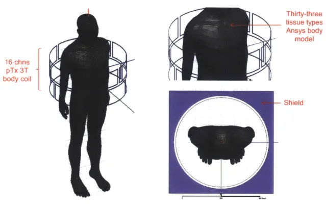
We have tested our approach on a pTx 3T body coil with 16 channels distributed in 2 rows (Figure 4-1). We used HFSS to compute the fields and the frequency response of this coil when loaded with the thirty-three tissue types Ansys body model. The coils were individually tuned (123.2MHz) and matched (-30dB) [26, 27].

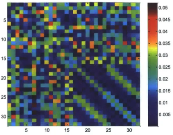
We used our algorithm to decouple this array. Figure 4-2 plots the norm of residuals depicting convergence (in about 150 - 200 iterations) of our algorithm for random initial guesses. The algorithm converges to distinct solutions depending on the initial guess. Non-uniqueness of the solution matrices allows specification of additional constraints such as limiting the capacitance and inductance values, and robustness of the solution matrix to external factors. Figure 4-3 shows the structure of one of the solution matrices

(jYj).

Y22(lower right block) has a specific structure

defined by the original coil assembly, where every coil is coupled to its neighbors. Figure 4-4 and 4-5 show the nearly perfect decoupling (0=no coupling, =perfect coupling) that results from application of the decoupling matrix (S12 was reduced

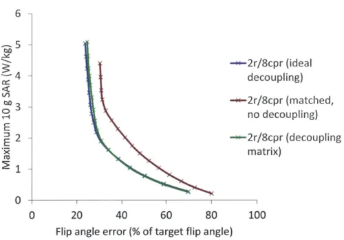
from -2dB to -200dB). Figure 4-6 and 4-7 show L-curves corresponding to RF-shimming pulses designed (i) with the coupled array, (ii) the array decoupled using our decoupling matrix and (iii) the array ideally decoupled in simulation. Least-square pulses were computed while explicitly constraining local SAR and power

[26].

The

L-Thirty-three tissue types Ansys body model 16 chns pTx 3T body coil Shield

Figure 4-1: EM simulation of a pTx coil with 16 channels distributed in 2 rows.

10 10 C,) 10 E 10 0 10 10-5 0 50 100 150 200 250 Iteration

10 15 20 25 30 1 u 10 zu o U 0.05 0.045 0.04 0.035 0.03 0.025 0.02 0.015 0.01 0.005

Figure 4-3: Magnitude of one of the possible decoupling matrices

1 0.8 0.6 0.4 0.2 0

Figure 4-4: Coupling coefficient matrix WITHOUT the decoupling network

curves (Figure 4-6 and 4-7) show that the coupled array was able to achieve a similar local SAR vs. fidelity tradeoff than the uncoupled ones however at the cost of greatly increased power consumption. There was no significant difference in performance between the ideally decoupled array and the array decoupled using our decoupling matrix. This also shows that the decoupling matrix produces mixed outputs that are non-degenerate and are therefore useful for pulse design (i.e., the singular values of the mixing matrix S2 1 are all of the same magnitude).

I

1 0.8 0.6 0.4 0.2 0

Figure 4-5: Coupling coefficient matrix WITH the decoupling network

6 7 --- 2r/8cpr (ideal decoupling) -*-2r/8cpr (matched, no decoupling) --- 2r/8cpr (decoupling matrix) 0 20 40 60 80 100

Flip angle error (% of target flip angle)

Figure 4-6: Local SAR vs. fidelity L- curves (slice-selective RF-shimming)

-5 4 c3 D 3 0 E 32 E 0

9000 -8000 3:7000 -3 6000 - -.- 2r/8cpr (ideal 8.5000 - decoupling) 4000 _-+x-2r/8cpr (matched, E no decoupling) :3000 -X -+m-2r/8cpr (decoupling 2000 ~matrix) 1000 -0 50 100

Flip angle error (% of target flip angle)

Figure 4-7: Power consumption of pulses shown in Figure 4-6

4.2

A 4-Channel Array

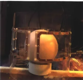
We fabricated a 4-channel parallel transmit head array (Figure 4-8). The array (tuned

and matched at 297.2MHz) demonstrates a significant coupling between the channels

as shown in Figure 4-9. This array requires an 8 port decoupling matrix. We enforced

the decoupling matrix to have the structure shown in Figure 4-10. We found that

this structure retained enough degrees-of-freedom needed to achieve good decoupling while reducing the number of reactive elements from N(2N+ 1) required to implement

an arbitrary decoupling matrix, down to N(N + 1) (N is the number of channels).

We designed two decoupling matrices with and without a robustness criterion. The non-robust decoupling matrix achieved ideal decoupling, Figure 4-12 (a), but had an extremely sharp frequency response. Imposing robustness constraints in the design of the decoupling matrix yielded a broader response, Figure 4-12 (b), making the circuit more tolerant to component value variations. Additionally, Figure 4-12 (c) shows that this robust design can be implemented in practice using standard C and L

values (see also Figure 4-11). Finally, we performed a sensitivity analysis of the final circuit with respect to small variations of the lumped element values, Figure 4-12

Figure 4-8: Picture of the coupled 4-channel 7T parallel transmit head array to be decoupled.

(d), by studying the output S-parameters of the array with the decoupling matrix,

when the capacitors and inductors values where swept in a -5% to +5% range. Our sensitivity analysis confirmed that the quality of the decoupling was indeed robust to variation of most of the lumped elements values within 5% This analysis also

revealed 2 crucial elements of the matrix, the values of which need to be known accurately to retain its performance (these may need to be implemented as variable capacitors and inductors).

4.3

Discussion

We have presented a framework to design a decoupling and matching network, a decoupling matrix, for parallel transmit arrays. Key advantages of our proposed framework are that it is generic, automatic and scalable. This means that the pro-posed decoupling strategy is independent of array's geometrical configuration and the number of channels. Such a matrix could be used to decouple transmit coils with many channels (i.e., > 16), which are difficult to decouple properly using existing

methods but have been shown to be beneficial for SAR reduction and manipulation of the transverse magnetization signal.

U) 0 --10 -20--40 280 290 300 310 Frequency (MHz) 320 330

Figure 4-9: S-parameters of the array without a decoupling matrix. Sjj indicates the reflection at port i, while Sij indicates the coupling between ports i and

j.

The decoupling is achieved at the cost of only a small insertion loss mainly due to the the parasitic loss of reactive lumped elements. A decoupling strategy is useful if its performance is robust to component value variations. We enforce this by searching for a decoupling matrix which is robust to variations via LI regularization.

PA

1

PA

₂

PA

₃

PA

₄

1Y

5

2

61

Y2

3

7

Y3 Y2 8 Y418

44

8

20 reactive elements

Figure 4-10: Schematic of the decoupling matrix. The elements Yj, indicate a reactive element connected between the nodes i and

j.

10 20 30

Capacitance (pF)

20 30

Inductance (nH)

40 50

Figure 4-11: Histograms of the calculated standard capacitors and inductors for the decoupling matrix 15 0 5 10 0AI E, 0 C.5 *0 3-- 2- 1-00 I

280 290 300 310 320 Frequency (MHz)

(a)

0 -10 -20 g -30 -40 -50 330 270 280 - - Ij ____ ____ I:-____ ____I₁L ~~~

S._

290 300 310 320 330 Frequency (MHz)

(b)

______ ______ _____iji _ 0.3v 0 _-E 0 C,) \i 290 300 310 320 330 Frequency (MHz) (c) 0.2 0. 0.1 0.

y

1

,

1 5 2 18

5

H

-5 0 Percentage Variation

(d)

Figure 4-12: (a) S-parameters of the array with the decoupling matrix S0st without

a robustness criterion. (b) S-parameters of the array with the decoupling matrix

Sost with a robustness criterion. (c) S-parameters of the robust matrix populated

with capacitors and inductors having only standard values. (d)Variation of the sum of all S-parameters (Frobenius norm of the output S-matrix) with respect to -5% to +5% variations of the lumped elements (1 curve per lumped element). The red curves indicate lumped elements that are the most critical for good performance of the decoupling matrix.

0 -50 -100 U) 150 -- siji _

Si,

0 -1C -2C -30 -4( U) 570 280 5 -200

0.357-Chapter 5

MRI Sensitivity Analysis

In this chapter we investigate the circuit level performance of an MRI coil with respect to arbitrary axial head position.

5.1

Purpose

For a given excitation mode, head model, and head position, the excitation efficiency over the entire brain shows good stability over a wide range of 7T MRI coils [28], when the arrays are properly designed (excitation efficiency is defined as Bl+v/VPv,

where B1+v is B1+ averaged over the brain and Pv is the power deposited in the

brain). In order to maintain stable transmit performance for a wide range of human head positions and sizes, care must be taken to avoid significant changes in the

dis-sipated energy that is wasted (transmit performance is defined as B1+V//Ptranmit,

where Ptransmit is the power transmitted to the coil). Energy wasting terms comprise:

the power radiated by the coils (Padiated); the inherent coil losses (Pinternai) produced

by lossy lumped elements (e.g. capacitors and inductors), by dielectrics and by con-ductors; and the power reflected by the entire coil (Peflected). It is important to note that once the coil geometry and fabrication design have been fixed, it is only possible to influence Preflected by circuit level optimization of selected components of the coil (e.g. tune and match capacitors, decoupling network, etc.). A mode and

a given set of excitation modes, head sizes and head positions. Finally, for a robust coil design it is crucial to be able to validate the performance of the coil at the circuit level for arbitrary axial head positions and head sizes within a given range.

Despite significant speed improvement in state-of-the-art commercial 3-D electro-magnetic (EM) field solvers, from a practical point of view only a few dozen complete

3-D EM simulations can be performed for any particular RF coil geometry. It is

thus impossible in practice to obtain the required 3-D EM data for a large number of arbitrary combinations of head positions and head sizes. Use of parameterized cir-cuit models, generated from S-parameter data calculated by a 3-D EM solver, should enable computation of circuit level MRI coil properties for arbitrary values of coil or head geometry parameters. This solution has been successfully applied for several integrated circuit applications

[301,

but not yet for MRI applications. The goals of this study were: a) to generate a parameterized circuit model from a set of 3-D EM simulations; and b) to perform circuit level performance analysis with respect to arbitrary head position and head size.

5.2

Method

A 3-D EM model of a previously constructed 7T MRI coil [31] was simulated. In

our 3-D EM model we used the precise dimensions and material electrical properties of the coil resonance elements. However, neither the RF cable traps, nor the coaxial cable interconnections were included in the 3-D EM numerical model domain. The loads utilized were the multi-tissue Ansys human body models, cut in the middle of

the torso: head #1 with scaling factors X = 0.9, Y = 0.9, Z = 0.9 (simulating an

average head), head #2 with scaling factors X = 0.85, Y = 0.85, Z = 0.9 (simulating

a small head), and head #3 with scaling factors X = 0.95, Y = 0.975, Z = 0.9

(simulating a large head). Each head was located at five axial positions so that the distance between the crown of the head and the transceiver top was 0, 20, 40, 50, and 60mm. We used the 3-D EM field solver HFSS (Ansys) to generate from the

fifteen initial non-parameterized models. In our initial non-parameterized model, the frequency response of each element in the S-parameter matrices was modeled using rational transfer functions of the form [32]:

H(s)= Rk + D. (5.1)

k=1 s ak

Here ak and Rk describe the poles and residues respectively, and K is the total number of poles used, which defines the model order. We took particular care to guar-antee that the circuit-level parameterized model generated is physically consistent. For instance, we ensured that the complex poles appeared in conjugate pairs and that all the poles were stable i.e. they had a negative real part (Rak < 0) regardless of the

values of the parameters. Using an optimization framework as described in

[32],

for each head position (i.e. 0mm, 20mm, 40mm, 50mm and 60mm) we generated initial non-parameterized models minimizing the mismatch of the frequency responses with the previously obtained HFSS data. We noted that the pole locations did not change significantly with respect to different head positions. In order to combine the initial non-parameterized models to generate a final parameterized model, we approximated the parameter dependence using multivariate polynomials. Our final parameterized model is of the form:

H(s, Z, H,) = Rk(Z, H +) + D(Z, Hs). (5.2)

k=1 s - ak

Here Rk(Z, Hs) and D(Z, Hs) are multivariate polynomials, Z is the head position and Hs defines the scaling factor. The model was finally implemented both as an hspice-netlist and as a Verilog-A module. In general, both of these interfaces are supported by all the major circuit simulators. However, we have observed that the Verilog-A format runs slower and may cause memory problems with a large number of ports. When our hspice-netlist model was incorporated within the circuit simulator as

4) 0 a-0. 0. 0. 0. 8 .head #3 6- - -- head #2 5- 3-30 40 50 60 70 80 90 100 Head position

Figure 5-1: Calculated dependency

a circuit object, the head size and location were represented by two object properties. This allows accurate and convenient sweeping in an arbitrary way of those parameters during the circuit level analysis.

5.3

Results and discussion

The error observed in the frequency response between the initial non-parameterized models and 3-D EM frequency response of correspondent geometries was less than 0.1% at coil operation (Larmor) frequency of 297.2MHz. No noticeable difference

was observed between the transceiver circuit level properties (e.g. Preflected)

com-puted directly from the HFSS S-parameter at the 15 given dataset combinations of parameter values and those computed from our parameterized circuit model, for 15 different combinations of head position and head size. Finally, Figure 5-1 shows the computed reflected power Preflected as a function of arbitrary intermediate values of

the axial head position. The values of the parameters for the initial individual 3-D

EM simulations were chosen manually based on our previous numerical investigation experience.

Chapter 6

Conclusion

We have presented a framework to automatically design decoupling matrices for pTx arrays with many channels (> 8). The algorithm optimally selects the component values of the decoupling matrix by enforcing reciprocity, passivity and the lossless-ness constraints on the network. The proposed framework also includes strategies to discover the underlying topology and structures for the decoupling matrix. We show that our algorithm converges and the decoupling matrix achieves near perfect

decoupling.

We have also generated parameterized models with a very large number of ports for sensitivity analysis of existing transmit arrays with respect to head positions. The parameterized models can be used to obtain any circuit level properties for arbitrary head positions within the given range.

Bibliography

[1]

Rainer Schneider, Bastien Gu6rin, Michael Hamm, Jens Haueisen, Elfar Adal-steinsson, Lawrence L Wald, and Josef Pfeuffer. Spatial Selective Excitation Performance of Parallel Transmission Using a 3x8 Z-Stacked RF Coil Array at

3T. In Proc. of 21st Annual Meeting and Exhibition of International Society for

Magnetic Resonance in Medicine. ISMRM, April 2013.

[2] Yudong Zhu. Parallel excitation with an array of transmit coils. Magnetic

Res-onance in Medicine, 51(4):775-784, 2004.

[3]

U Katscher, P Vernickel, and J Overweg. Basics of RF power behaviour in

parallel transmission. Methods, 1:3, 2005.

[4]

Peter Ullmann, Sven Junge, Markus Wick, Frank Seifert, Wolfgang Ruhm, and Jiirgen Hennig. Experimental analysis of parallel excitation using dedicated coil setups and simultaneous RF transmission on multiple channels. Magnetic

reso-nance in medicine, 54(4):994-1001, 2005.

[5] Y Zhu, R Watkins, R Giaquinto, C Hardy, G Kenwood, S Mathias, T Valent,

M Denzin, J Hopkins, W Peterson, and Others. Parallel excitation on an eight transmit-channel MRI system. In Proceedings of the 13th Annual Meeting of

ISMRM, Miami Beach, FL, USA, page 14, 2005.

[6]

Michael A Ohliger and Daniel K Sodickson. An introduction to coil array design for parallel MRI. NMR in Biomedicine, 19(3):300-315, 2006.

[7]

Kawin Setsompop, Lawrence L Wald, Vijayanand Alagappan, Borjan Gagoski, Franz Hebrank, Ulrich Fontius, Franz Schmitt, and Elfar Adalsteinsson. Parallel RF transmission with eight channels at 3 Tesla. Magnetic resonance in medicine,

56(5):1163-1171, 2006.

[8]

Hon Tat Hui. Decoupling methods for the mutual coupling effect in antenna arrays: a review. Recent Patents on Engineering, 1(2):187-193, 2007.

[91 P B Roemer, W A Edelstein, C E Hayes, S P Souza, and 0 M Mueller. The

NMR phased array. Magnetic resonance in medicine, 16(2):192-225, 1990.

[10] Jianmin Wang and Others. A novel method to reduce the signal coupling of

surface coils for MRI. In Proceedings of the

4th

Annual Meeting of ISMRM, New York, NY, USA, page 1434, 1996.

[11] G R Duensing, H R Brooker, and J R Fitzsimmons. Maximizing signal-to-noise

ratio in the presence of coil coupling. Journal of Magnetic Resonance, Series B,

111(3):230-235, 1996.

[12] Bing Wu, Peng Qu, Chunsheng Wang, Jing Yuan, and Gary X Shen. Inter-connecting L/C components for decoupling and its application to low-field open MRI array. Concepts in Magnetic Resonance Part B: Magnetic Resonance

En-gineering, 31(2):116-126, 2007.

[13]

M Kozlov, R Turner, and N Avdievich. Investigation of decoupling between

MRI array elements. In Microwave Conference (EuMC), 2013 European, pages

1223-1226, October 2013.

[14] V Alagappan, G C Wiggins, A Potthast, K Setsompop, E Adalsteinsson, and L L Wald. An 8 channel transmit coil for transmit SENSE at 3T. In Proceedings

of the 14th Annual Meeting of ISMRM, Seattle, WA, USA, 2006.

[15]

J Jevtic. Ladder networks for Capacitive Decoupling in Phased-Array Coils. In

Proc. of Annual Meeting and Exhibition of International Society for Magnetic Resonance in Medicine. ISMRM, April 2001.

[161 Hans Steyskal and Jeffrey S Herd. Mutual coupling compensation in small array

antennas. IEEE Transactions on Antennas and Propagation, 38:1971-1975, 1990.

[17] P Vernickel, C Findeklee, J Eichmann, and I Graesslin. Active digital

decou-pling for multi-channel transmit MRI Systems. In Proc. of Annual Meeting and

Exhibition of International Society for Magnetic Resonance in Medicine, 2007.

[18] P P Stang, M G Zanchi, A Kerr, J M Pauly, and G C Scott. Active Coil

Decoupling by Impedance Synthesis using Frequency-Offset Cartesian Feedback. In Proc. of Annual Meeting and Exhibition of International Society for Magnetic

Resonance in Medicine, number 332, page 332. ISMRM, May 2011.

[19] D C Youla. Direct single frequency synthesis from a prescribed scattering matrix.

Circuit Theory, IRE Transactions on, 6(4):340-344, 1959.

[201 J Bach Andersen and Henrik Hass Rasmussen. Decoupling and descattering net-works for antennas. IEEE Transactions on Antennas and Propagation, 24:841-846, 1976.

[211

W Preston Geren, Clifford R Curry, and Jonny Andersen. A practical technique for designing multiport coupling networks. Microwave Theory and Techniques,

IEEE Transactions on, 44(3):364-371, 1996.

[22] Jeffery C Allen and John W Rockway. Characterizing Optimal Multiport Match-ing Transformers. _{Circuits, Systems, and Signal Processing, 31(4):1513-1534,} 2012.

[23] Ray F Lee, Randy 0 Giaquinto, and Christopher J Hardy. Coupling and

decou-pling theory and its application to the MRI phased array. Magnetic resonance

in medicine, 48(1):203-213, 2002.

[24]

Z Mahmood, B Guerin, E Adalsteinsson, L L Wald, and L Daniel. An Auto-mated Framework to Decouple pTx Arrays with Many Channels. In Proc. of 21st

Annual Meeting and Exhibition of International Society for Magnetic Resonance in Medicine. ISMRM, April 2013.

[25] Z Mahmood, B Guerin, B Keil, E Adalsteinsson, L L Wald, and L Daniel. Design

of a Robust Decoupling Matrix for High Field Parallel Transmit Arrays. In Proc.

of 22nd Annual Meeting and Exhibition of International Society for Magnetic Resonance in Medicine. ISMRM, May 2014.

[26] Guerin B., E. Adalsteinsson, and L. Wald. Local sar reduction in multi-slice ptx

via aAIJsar hoppingaAi between excitations. In Proceedings of the 9th Annual

Meeting of ISMRM, Melbourne, Australia, volume 20, page 2612, 2012.

[27] M. Kozlov and R. Turner. Fast mri coil analysis based on 3-d electromagnetic

and rf circuit co-simulation. Journal of Magnetic Resonance, 200(1):147-152,

2009.

[28] M. Kozlov and R. Turner. Analysis of rf transmit performance for a multi-row

multi-channel mri loop array at 300 and 400 mhz. In Microwave Conference

Proceedings (APMC), 2011 Asia-Pacific, pages 1190-1193. IEEE, 2011.

[29] M. Kozlov and R. Turner. Multi-mode optimization of a near-field array. In 42nd

European Microwave Conference, pages 309-312, 2012.

[301

Z. Mahmood. Parameterized modeling of multiport passive circuit blocks. PhD

thesis, Massachusetts Institute of Technology, 2010.

[31] Z. Zuo and et al. An elliptical octagonal phased-array head coil for multi-channel

transmission and reception at 7t. In 20th ISMRM, page 2804, 2012.

[32] Z. Mahmood, R. Suaya, and L. Daniel. An efficient framework for passive

com-pact dynamical modeling of multiport linear systems. In Design, Automation &

Test in Europe Conference & Exhibition (DATE), 2012, pages 1203-1208. IEEE,