HAL Id: hal-03094573
https://hal.sorbonne-universite.fr/hal-03094573
Submitted on 4 Jan 2021
HAL is a multi-disciplinary open access
archive for the deposit and dissemination of
sci-entific research documents, whether they are
pub-lished or not. The documents may come from
teaching and research institutions in France or
abroad, or from public or private research centers.
L’archive ouverte pluridisciplinaire HAL, est
destinée au dépôt et à la diffusion de documents
scientifiques de niveau recherche, publiés ou non,
émanant des établissements d’enseignement et de
recherche français ou étrangers, des laboratoires
publics ou privés.
Manuel Schlund, Veronika Eyring, Gustau Camps-valls, Pierre Friedlingstein,
Pierre Gentine, Markus Reichstein
To cite this version:
Manuel Schlund, Veronika Eyring, Gustau Camps-valls, Pierre Friedlingstein, Pierre Gentine, et
al..
Constraining Uncertainty in Projected Gross Primary Production With Machine Learning.
Journal of Geophysical Research: Biogeosciences, American Geophysical Union, 2020, 125 (11),
�10.1029/2019jg005619�. �hal-03094573�
Manuel Schlund1 , Veronika Eyring1,2 , Gustau Camps‐Valls3 , Pierre Friedlingstein4,5, Pierre Gentine6,7 , and Markus Reichstein8,9
1Deutsches Zentrum für Luft‐ und Raumfahrt (DLR), Institut für Physik der Atmosphäre, Oberpfaffenhofen, Germany, 2Institute of Environmental Physics (IUP), University of Bremen, Bremen, Germany,3Image Processing Laboratory (IPL),
Universitat de València, València, Spain,4College of Engineering, Mathematics and Physical Sciences, University of Exeter, Exeter, UK,5LMD/IPSL, ENS, PSL Université, Ecole Polytechnique, Institut Polytechnique de Paris, Sorbonne
Université, CNRS, Paris, France,6Department of Earth and Environmental Engineering, Columbia University, New York, NY, USA,7Earth Institute and Data Science Institute, Columbia University, New York, NY, USA,8Department of
Biogeochemical Integration, Max Planck Institute for Biogeochemistry, Jena, Germany,9Michael‐Stifel‐Center Jena for Data‐driven and Simulation Science, Jena, Germany
Abstract
The terrestrial biosphere is currently slowing down global warming by absorbing about 30% of human emissions of carbon dioxide (CO2). The largestflux of the terrestrial carbon uptake is gross primary production (GPP) defined as the production of carbohydrates by photosynthesis. Elevated atmospheric CO2concentration is expected to increase GPP (“CO2fertilization effect”). However, Earth system models (ESMs) exhibit a large range in simulated GPP projections. In this study, we combine an existing emergent constraint on CO2fertilization with a machine learning approach to constrain the spatial variations of multimodel GPP projections. In afirst step, we use observed changes in the CO2seasonal cycle at Cape Kumukahi to constrain the global mean GPP at the end of the 21st century (2091–2100) in Representative Concentration Pathway 8.5 simulations with ESMs participating in the Coupled Model Intercomparison Project Phase 5 (CMIP5) to 171 ± 12 Gt C yr−1, compared to the unconstrained model range of 156–247 Gt C yr−1. In a second step, we use a machine learning model to constrain gridded future absolute GPP and gridded fractional GPP change in two independent approaches. For this, observational data are fed into the machine learning algorithm that has been trained on CMIP5 data to learn relationships between present‐day physically relevant diagnostics and the target variable. In a leave‐one‐model‐out cross‐validation approach, the machine learning model shows superior performance to the CMIP5 ensemble mean. Our approach predicts an increased GPP change in northern high latitudes compared to regions closer to the equator.Plain Language Summary
About a quarter of human emissions of carbon dioxide (CO2) is absorbed by vegetation and soil on the Earth's surface and hence does not contribute to global warming caused by CO2in the atmosphere. Thus, in order to better define the remaining carbon budgets left to meet particular warming targets like the 1.5°C of the Paris Agreement, it is important to accurately quantify the carbon uptake by plants in the future. Currently, this is modeled by Earth system models yet with great uncertainties. In this work, we present an alternative machine learning approach to reduce spatial uncertainties of vegetation carbon uptake in future climate projections using observations of today's conditions.1. Introduction
The response of the terrestrial carbon cycle to changes in atmospheric CO2 and climate is a major source of uncertainty in climate projections (Bodman et al., 2013; Booth et al., 2012; M. Collins et al., 2013). Future terrestrial carbon sensitivity is mainly driven by two feedback mechanisms: the concentration‐carbon and the climate‐carbon feedbacks (M. Collins et al., 2013; Friedlingstein et al., 2006; Gregory et al., 2009). The first one is connected to the CO2 fertilization effect (Walker et al., 2020) where elevated atmospheric CO2 concentrations increase photosynthesis rates and generally lead to a higher terrestrial carbon uptake, thus constituting a negative feedback. The second one, the climate‐carbon feedback, is driven by temperature and precipitation changes leading to a smaller land ©2020. The Authors.
This is an open access article under the terms of the Creative Commons Attribution License, which permits use, distribution and reproduction in any medium, provided the original work is properly cited.
Key Points:
• An emergent constraint on CO2 seasonal cycle amplitude changes reduces uncertainties in global mean gross primary production projections
• A machine learning model with multiple predictors can further constrain the spatial distribution of gross primary production • High‐latitude ecosystems show
higher gross primary production increase over the 21st century compared to regions closer to the equator Supporting Information: • Supporting Information S1 Correspondence to: M. Schlund, [email protected] Citation:
Schlund, M., Eyring, V., Camps‐Valls, G., Friedlingstein, P., Gentine, P., & Reichstein, M. (2020). Constraining uncertainty in projected gross primary production with machine learning.
Journal of Geophysical Research: Biogeosciences, 125, e2019JG005619. https://doi.org/10.1029/2019JG005619 Received 19 DEC 2019
Accepted 18 SEP 2020
carbon uptake because of increased temperature and water stress on photosynthesis and higher ecosys-tem respiration costs, as well as increasedfire frequency.
The terrestrial biosphere currently absorbs about 30% of the total anthropogenic CO2 emissions (Friedlingstein et al., 2019), yet whether that benefit will perdure in the future remains unclear (Friedlingstein et al., 2006). Accurate prediction of future carbon uptake is, however, of paramount impor-tance to accurately determine the allowable CO2emissions to meet particular temperature targets, such as the 1.5°C of the Paris Agreement (Matthews et al., 2009; UNFCCC, 2015). One way to quantify future terres-trial carbon uptake is via the use of land surface models within Earth system models (ESMs). Here we use ESM outputs from thefifth phase of the Coupled Model Intercomparison Project (CMIP5) (Taylor et al., 2012). However, since this model ensemble shows a large spread in the evolution of the land carbon sink (Ciais et al., 2013), a careful statistical evaluation and refinement of the multimodel mean and its uncertainty is required.
A prominent method to constrain future model estimates using observations is the so‐called “emergent con-straint” approach (Allen & Ingram, 2002), which is based on an intermodel relationship between an obser-vable quantity in the past climate and a projected quantity of the future climate. Emergent constraints have already been successfully applied to carbon cycle processes (Cox et al., 2013; Wenzel et al., 2014; Wenzel, Cox, et al., 2016) and are thought to be a promising technique to reduce uncertainties in climate model ensemble output (Eyring et al., 2019). However, two limitations of this technique are the use of a single (globally or regionally averaged) variable per climate model and the assumption of a linear relationship between the observed and the target variable. Other methods involve a weighting of the multimodel average based on model performance relative to observations (Knutti et al., 2017; Sanderson et al., 2017), including process‐oriented approaches like the multiple diagnostic ensemble regression (MDER) (Karpechko et al., 2013; Senftleben et al., 2019; Wenzel, Eyring, et al., 2016).
In this paper, we introduce a new two‐step approach that utilizes aspects of both aforementioned techniques in combination with a supervised machine learning algorithm to constrain uncertainties in multimodel pro-jections of gross primary production (GPP) with observations. In thefirst step, we apply an existing emergent constraint on CO2fertilization (Wenzel, Cox, et al., 2016) to constrain ESMs' responses to rising atmospheric CO2 concentration using observations of the increase of the CO2 seasonal cycle amplitude at Cape Kumukahi, Hawaii (Keeling et al., 2005). In a second step, we introduce a supervised machine learning algo-rithm based on boosting trees (Friedman, 2001) to learn an empirical spatial relationship that links grid‐wise future GPP to historical processes relevant to its simulation under present‐day conditions. In combination with observational products of the predictors, that relationship can be used to further constrain uncertainties in the projected spatial maps of GPP at the end of the 21st century in the Representative Concentration Pathway (RCP) 8.5 scenario (Riahi et al., 2011). We examine both constraining the absolute GPP and the fractional change in GPP as two independent approaches and target variables. Unlike univariate linear regression used in the MDER algorithm, the proposed Gradient Boosted Regression Tree (GBRT) algorithm is able to handle multiple predictors and copes with nonlinearities in the data. GBRT is a well‐known and successful tool used for interpolation, classification and prediction in other fields of data science and engineering (De'ath, 2007; Elith et al., 2008). In the context of climate science, GBRT was recently applied to identify the key drivers of spatial variations of the ratio of plant transpiration to total terrestrial evapotran-spiration in ESMs (Lian et al., 2018).
In this study, we combine an emergent constraint approach with the GBRT algorithm to reduce uncertain-ties in projected GPP. Section 2 provides an overview of the methods and data used in this paper. The results are presented in section 3, and section 4 closes with a summary and discussion.
2. Methods and Data
Here we briefly describe the methods and data used in this study. Section 2.1 reviews the method of a pre-viously published emergent constraint on CO2fertilization from Wenzel, Cox, et al. (2016) that we apply here to our study to rescale the climate model output (Step 1). This includes a discussion of the caveats that are associated with this emergent constraint that attributes changes in the observed increase in the CO2 sea-sonal cycle amplitude at Cape Kumukahi entirely to the increase in atmospheric CO2concentration, yet
other studies provide indications that part of this increase is due to climate and land use changes (Bastos et al., 2019; Forkel et al., 2016; Piao et al., 2018; Zhao et al., 2016). In section 2.2 the machine learning technique used in Step 2 to constrain gridded GPP projections is presented. Figure 1 shows an overview of our two‐step approach. Section 2.3 describes how uncertainty and predictive skill are quantified.
A complete list of all CMIP5 models used in this study is given in supporting information Table S1. To apply the emergent constraint in Step 1, we need emission‐driven CMIP5 simulations. The number of ESMs included is therefore seven, as in Wenzel, Cox, et al. (2016). More details on the methods and the experimen-tal setup are given as supporting information.
2.1. Constraining the CO2Fertilization Effect (Step 1)
In this section, we present the observational emergent constraint on the CO2fertilization effect by Wenzel, Cox, et al. (2016) which we use to globally rescale the models for their individual bias in the sensitivity of GPP to an increase in atmospheric CO2concentration. Our objective here is to present a general methodol-ogy and suggest further improvements upon this constraint that could be used in the future. Wenzel, Cox, et al. (2016) showed a correlation between the increase in the CO2seasonal cycle amplitude simulated by models and the projected CO2‐fertilization. When combined with the observed trends in the CO2seasonal cycle amplitude, the fractional GPP change at the time of CO2doubling relative to preindustrial conditions in a biogeochemically coupled simulation where the atmospheric CO2concentration increases by 1% per year (1%BGC) was constrained. The predictor in this study is the sensitivity of the CO2seasonal cycle ampli-tude to rising atmospheric CO2concentrations, defined as the slope of the linear regression between the CO2 seasonal cycle amplitude and the annual mean atmospheric CO2concentrations (see Figure S1 for details). The emergent constraint is physically motivated by the hypothesis that increasing terrestrial GPP is a main driver for the observed changes in the CO2seasonal cycle amplitude (Gray et al., 2014; Keeling et al., 1996; Zhao & Zeng, 2014). This hypothesis is based on the fact that the seasonal cycle in atmospheric CO2 concen-tration originates from photosynthesis and decomposition processes: in summer, photosynthesis removes CO2from the atmosphere; in winter, additional CO2is added to the atmosphere due to the decomposition Figure 1. Schematic illustration of our two‐step approach. In Step 1 an emergent constraint by Wenzel, Cox, et al. (2016)
is used to constrain the global mean fractional GPP change over the 21st century. Moreover, this constraint is used to rescale two different gridded target variables: absolute GPP at the end of the 21st century and fractional GPP change over the 21st century. In Step 2, a machine learning model is used to constrain these two target variables (Step 2a: absolute GPP; Step 2b: fractional GPP change) in two independent approaches.
of organic matter (Keeling et al., 1995). Thus, CO2fertilization leads to an increase of the CO2seasonal cycle amplitude due to increased CO2removal from the atmosphere. We note that this emergent constraint impli-citly assumes that there is no temperature‐driven increase in respiration over time. Therefore, this approach most likely overestimates the true sensitivity of GPP to an increase in the atmospheric CO2concentration. However, we note that this emergent constraint is not undisputed. In other studies, the observed change in the CO2seasonal cycle amplitude has been attributed to other factors. Using a dynamic global vegetation model, Forkel et al. (2016)find that the increase in the CO2seasonal cycle amplitude above 40°N is mainly driven by the response of plants to global warming instead of CO2. Similarly, Piao et al. (2018) show that ele-vated atmospheric CO2concentration and climate change equally contribute to the increase in the CO2 sea-sonal cycle in northern high latitudes with additional smaller contributions from air‐sea carbon fluxes and land use changes. For their analysis, Piao et al. (2018) used CO2records from 26 stations and nine terrestrial ecosystem models. An evaluation of two atmospheric inversions and 11 land surface models shows contrast-ing effects of CO2fertilization (positive) and global warming (negative) on the CO2seasonal cycle amplitude increase in northern high latitudes with negligible contributions from land use changes (Bastos et al., 2019). A further study by Zhao et al. (2016)finds that for seven out of nine dynamic vegetation models, the CO2 fertilization effect is the strongest driver for the observed changes in the CO2seasonal cycle amplitude, while the two remaining models equally attribute this to CO2fertilization, climate change and land use changes. Moreover, Winkler, Myneni, and Brovkin (2019) discuss limitations of carbon cycle emergent constraints related to the calculation of the predictor from observation‐based data and the intermodel relationship. As a case study, they adopt a further emergent constraint by Winkler, Myneni, Alexandrov, and Brovkin (2019) that uses the response of the leaf area fraction to ambient CO2instead of the CO2seasonal cycle amplitude sensitivity to constrain the GPP increase in the northern high latitudes. Furthermore, it has been shown that the CMIP5 models (Graven et al., 2013) and the TRENDY dynamic vegetation models (Thomas et al., 2016) greatly underestimate long‐term changes in the CO2seasonal cycle which questions their ability to attribute changes in the CO2seasonal cycle to different contributors. Nevertheless, we empha-size that we here present a generic methodology and use the results of an existing emergent constraint. Our proposed framework is universal and could be based on other emergent constraints in the future.
In contrast to Wenzel, Cox, et al. (2016), instead of idealized simulations we apply the presented emergent constraint on the emission‐driven RCP 8.5 simulation (Riahi et al., 2011) and examine whether it still holds for this simulation where forcings other than CO2also change. Moreover, we consider the global mean GPP change instead of the GPP change in the northern extratropics as in Wenzel, Cox, et al. (2016). Due to the strong annual mixing of CO2in the atmosphere, the change in the CO2seasonal cycle amplitude at Cape Kumukahi is representative for the whole globe. Thus, we apply this emergent constraint to the global mean GPP change. However, we note that this approach might introduce errors since the CO2fertilization effect could be different for tropical and extratropical ecosystems due to nutrient limitations and the temperature dependence of Rubisco kinetics (Crafts‐Brandner & Salvucci, 2000) in the tropics. Nevertheless, we argue that we can use the constraint if the emergent relationship still holds within our considered framework (the RCP 8.5 scenario simulated by the CMIP5 models).
Therefore, our target variable in Step 1 is the global mean GPP change over the 21st century f in the RCP 8.5 scenario, which is calculated from the 10 year mean GPP at the end of the 21st century in the emission‐driven fully coupled RCP 8.5 simulations (2091–2100) and the 10 year mean GPP at the end of the 20th century (1991–2000) in the emission‐driven historical simulation:
f¼GPPð2091–2100Þ
GPPð1991–2000Þ− 1 (1)
This variable is given as a percentage, where negative values correspond to a decrease in GPP, positive values to an increase in GPP and a value of 0% to no GPP change. The CO2amplitude sensitivity is calcu-lated for the years 1979–2019, which is the full available time range for the observed CO2 at Cape Kumukahi (Keeling et al., 2005). Similar to Wenzel, Cox, et al. (2016), we extract the observed CO2 ampli-tude from smoothed atmospheric CO2 concentrations (using a stiff cubic spline function plus a four‐harmonics functions with linear gain) as provided by Keeling et al. (2005). For the CMIP5 models,
the respective grid cell closest to Cape Kumukahi (19.5°N, 154.8°W) is extracted. Additionally, the emission‐driven historical simulations are extended with the emission‐driven RCP 8.5 simulations for the years 2006 to 2019. More details including an illustration of this calculation are shown in Figure S1. Since the global constraint above cannot be used directly as a predictor in the machine learning approach which operates on gridded values (see section 2.2), we use it asfirst step to globally rescale the ESM output. This importantfirst step allows us to constrain the large uncertainty in the global CO2fertilization effect of the CMIP5 models. In this study, two different gridded target variables are examined: the monthly climatol-ogy of future absolute GPP at the end of the 21st century (2091–2100) in the RCP 8.5 scenario (see Step 2a) and the fractional GPP change over the 21st century as defined in Equation 1 (see Step 2b). The global rescal-ing of the gridded target variables works as follows: let fmbe the global mean fractional GPP change over the 21st century of ESM m, f′ the constrained value of the global mean fractional GPP change and ym,ithe target variable of ESM m. Then, we define the rescaled target variable y′m,iby
y′m; i¼ ym; i·ff′ m
; (2)
where the index i counts over all grid cells (and months when absolute GPP is used as target variable in Step 2a) and m refers to the ESM (m∈ {1,2,…,7}). Thus, values for the individual grid cells/months are rescaled by a factor that is determined by the ratio between the models' global mean GPP change and the constrained global mean GPP change derived from the Wenzel, Cox, et al. (2016) emergent constraint using the observed change in the CO2cycle amplitude. Models that simulate a too high global mean GPP change are nudged toward smaller values and vice versa. The rescaled target variables are then fed into the machine learning model (Step 2) presented in the following section. We note that this global rescaling assumes that the relative biases in the fractional GPP change of the individual ESMs are constant over the whole globe.
2.2. Gradient Boosted Regression Trees (Step 2)
For Step 2 we use the GBRT algorithm tofind an optimal regression function F relating the target variable y to a set of K predictorsx = (x(1), x(2),…, x(K)) (“features” or “covariates”) such that the predicted target vari-able is given byby ¼ F xð Þ (De'ath, 2007; Elith et al., 2008; Friedman, 2001, 2002). Its basic elements are deci-sion trees, which use binary splits of the input data to create decideci-sion rules. Due to their simple nature, decision trees are easy to interpret but cannot be used to create satisfying predictions for very complex data sets. This issue can be overcome by a technique called“boosting” (Freund & Schapire, 1996). Boosting itera-tively improves the performance of“weak learners” (in our case decision trees) in the following way: At first, a single decision tree isfitted to a randomly selected subsample of the training data {(xi, yi)} (using a prede-fined loss function, e.g., the mean square error). Then, further decision trees are linearly added to the regres-sion function F (scaled by a regularization parameterυ ≪ 1 called “learning rate”) and the model is fitted again in the same manner. This ensures that the prediction for poorly modeled training points in the begin-ning will gradually improve during the traibegin-ning. The whole procedure is repeated until the loss function does not improve anymore, as evaluated on an independent validation data set. Relevant hyperparameters of this algorithm (maximum number of decision trees, maximum depth of the decision trees, learning rate, and the subsample ratio) are optimized byfivefold cross‐validation using the training data. More details on the GBRT algorithm can be found in Text S2.
A convenient way to evaluate and interpret GBRT models (or other statistical models in general) is to iden-tify the most relevant predictors. Globally, this so‐called “feature importance” is closely related to the num-ber of appearances of a feature in the different decision trees that set up the GBRT model (Friedman, 2001). To evaluate the feature importance regionally (for the different grid cells), we use a model distillation tech-nique called LIME (“local interpretable model‐agnostic explanations”), which approximates the GBRT model with a local linear regression model for each grid cell (Ribeiro et al., 2016). The corresponding linear coefficients bkfor each feature x(k)constitute a good proxy to the model's Jacobian ∂y
∂xð Þk, which is difficult to compute explicitly for this particular machine learning model. Thus, features with high (low) absolute bk have a high (low) impact on the local prediction of the target variable y.
As already described in the previous section, we analyze two different target variables in this study: the monthly climatology of absolute GPP at the end of the 21st century (Step 2a) and the fractional GPP change over the 21st century (Step 2b). A schematic representation of Step 2a is shown in Figure 2. The target vari-able y for the machine learning model is the rescaled monthly climatology of future GPP at the end of the 21st century (2091–2100) in the RCP 8.5 scenario given by Equation 2. We relate this target variable to sev-eral process‐oriented diagnostics x of the past climate (historical simulation) listed in Table 1. A single train-ing point (xi, yi) for the supervised machine learning algorithm corresponds to the set of the aforementioned diagnostics evaluated on a single grid cell/month of a single climate model (see colored dots in Figures 2a and 2b). Step 2b differs from Step 2a only in the target variable used. Both steps are independent approaches and are evaluated separately.
The main part of Steps 2a and 2b each consist of two phases. In thefirst phase (training of the algorithm), we build a statistical model based on the empirical relationship between observable process‐oriented variables of the present‐day climate and future GPP in the CMIP5 ensemble (see gray plane in Figures 2a and 2b). This has aflavor similar to the MDER algorithm, which is a climate model weighting method that uses a multi-variate linear regression algorithm to constrain multimodel climate projections of a target variable with observations (Karpechko et al., 2013; Senftleben et al., 2019; Wenzel, Eyring, et al., 2016). However, in con-trast to the original MDER algorithm, our multivariate GBRT approach is able to handle multiple predictors with nonlinear dependencies. Moreover, instead of considering a single globally or regionally averaged value per climate model, our approach uses spatiotemporally gridded data for every ESM in the ensemble. This dramatically increases the available number of training data (even if they are not statistically independent) and uniquely enables the statistical model to identify and exploit regional processes. Furthermore, the large training database allows us to perform extensive out‐of‐sample testing, which is crucial to ensure the model robustness.
In the second phase (predicting with the trained GBRT model), we use observational data products to con-strain the RCP 8.5 CMIP5 projection of GPP. To do this, observational data for all predictorsx of the histor-ical climate (for every grid cell/month) are fed into the trained GBRT model in order to get a spatially constrained projection of GPP (see black dots in Figure 2b). Similar to the MDER algorithm, our approach assumes that there exists an intermodel relationship between the predictors and the target variable which also holds for the true climate. This assumption may seem weak atfirst glance, but compared to the assump-tion of tradiassump-tional weighting approaches (models that are better in simulating the present‐day climate are also better in simulating the future climate and vice versa), the MDER assumption is more reasonable and allows correcting models instead of just weighing (Karpechko et al., 2013). Following other MDER stu-dies (Karpechko et al., 2013; Senftleben et al., 2019; Wenzel, Eyring, et al., 2016), we also select diagnostics as predictor variablesx that are related to GPP‐relevant processes (see Table 1 for detailed physical explana-tions of the links between the predictors and GPP).
The raw CMIP5 and observation‐driven data sets are preprocessed before entering the machine learning algorithm (see Text S1). In particular, increases greater than 300% in the fractional GPP change that is used as target variable in Step 2b are removed. These unrealistically high values (making up about 5.9% of the data) occur in places with very small absolute GPP values in the historical simulation that are used in the denominator of the derivation of the fractional GPP change (see Equation 1). In addition, we randomly select 25% of the training data and use it as hold‐out test data. This data set is excluded from the training and can therefore be used for an independent validation of our statistical model.
2.3. Assessment of Uncertainty and Predictive Skill
The estimation of the standard prediction error (SPE) for the GBRT models needs to consider three sources of uncertainty: the uncertainty of the machine learning model itself, the uncertainty in the rescaling of the target variable (see Equation 2) and the uncertainty in the input data, that is, errors in the observation‐based products. First, the SPE of the GBRT model itself (i.e., uncertainty in the position of the gray plane in Figures 2a and 2b) is estimated as the root‐mean‐square error of predictions (RMSEP), that is, the root‐ mean‐square error (RMSE) between the predicted and true values of the independent hold‐out test data set (Bishop, 2006). This approach is justified when the distribution of residuals is unbiased (see Text S4), in which case the RMSEP equals the standard deviation of the residuals (which we interpret as error). Figure S2 shows that this is approximately correct.
(a)
(b)
(c)
Figure 2. Schematic illustration of our machine learning approach to constrain projected absolute GPP (Step 2a). (a) In
thefirst phase of the algorithm (training phase), the model is fitted to the training data interpolating the empirical (nonlinear) relationship between two process‐oriented diagnostics of the past climate {x(1), x(2)} and (rescaled) future GPP (gray plane). The dots show the training points for the supervised machine learning algorithm, each of them representing a single grid cell/month of a single climate model (the different colors correspond to different climate models). (b) In the second phase, observation‐based values of the diagnostic (black dots) are fed into the fitted machine learning model to constrain GPP for every grid cell/month to a value which best agrees with the observations. (c) For an independent validation of our method, we use an out‐of‐sample testing setup based on a leave‐one‐model‐out cross‐validation approach, that is, by testing on one climate model left out. For this, we create a data set with known ground truth by excluding a single climate model from the ensemble in the training phase and using it as input in the prediction phase. This allows us to evaluate the root‐mean‐square error between the predicted and the true values, yielding the so‐called root‐mean‐square error of prediction (RMSEP). By repeating this whole process for all climate models, we create a distribution of RMSEPs and compare it to different statistical models. The schematic illustration of Step 2b differs only in the target variable used (fractional GPP change instead of absolute GPP).
The SPE of the GBRT model can be understood as combined error due to the internal variability of the cli-mate system, the different model responses within the clicli-mate model ensemble to forcing and the incom-plete description of the climate system with the limited number of variables used as input features. Second, the uncertainty in the rescaling is simply assessed as the uncertainty given by the emergent con-straint from Step 1. Finally, the uncertainty in the observation‐based data (i.e., uncertainty in the position of the black dots in Figure 2b) is assessed by error propagation. The necessary sensitivities of the target vari-able to the various predictors for each grid cell/month are given by the linear coefficients bkgiven by the LIME approach introduced in section 2.2. All sources of uncertainty are assumed independent and are com-bined by adding the squared errors, yielding a single estimate of the SPE for each grid cell/month. Further details on the calculation of errors are given in Text S3.
The predictive power of the GBRT algorithm and its robustness is assessed using a leave‐one‐model‐out cross‐validation approach (see Figure 2c). This is also known as “pseudoreality” or “model‐as‐truth” approach in climate sciences (de Elia et al., 2002; Karpechko et al., 2013). For this, a single climate model is removed from the multimodel ensemble and considered as being the true climate. Our statistical model is thenfitted on all remaining climate models and a prediction for the “true” model is created. This allows a simple evaluation of the predictive power by calculating the RMSEP. The whole process is repeated for every climate model of the ensemble in order to get a distribution of RMSEPs. Since this approach is not lim-ited to GBRT, it allows a simple comparison of the predictive skill of different statistical models. We compare the GBRT model to the simple CMIP5 multimodel mean and a least absolute shrinkage and selection opera-tor (LASSO) model. The LASSO model (Tibshirani, 1996) is an extended linear regression model that regu-larizes the least squares solution with a L1‐penalty term. In contrast to the ordinary least square regression, the LASSO model promotes sparse solutions (i.e., only a few nonzero coefficients/weights), which acts as an intrinsic feature selection and acts as an effective way to combat overfitting induced by collinearity.
3. Results
3.1. Constraining Global Mean GPP Projections (Step 1)
In Wenzel, Cox, et al. (2016), the observed atmospheric CO2concentration at Cape Kumukahi, Hawaii (KUM; 19.5°N, 154.8°W) (Keeling et al., 2005) was used to constrain the GPP change in the 1%BGC run resulting from a doubling of atmospheric CO2 concentrations to 32 ± 9% for extratropical ecosystems (30–90°N). As mentioned in section 2.1, we argue that due to the strong annual mixing of CO2in the atmo-sphere, this emergent constraint can also be applied to the global mean GPP change if the emergent relation-ship holds. In order to test this, wefirst use the idealized CMIP5 simulations that were analyzed by Wenzel, Cox, et al. (2016) to calculate the emergent constraint (Figure 3a). The relationship is statistically significant at a 5% significance level (R2 = 0.79,p = 0.007) and predicts a constrained global mean GPP change of Table 1
Process‐Oriented Diagnostics (“Predictors” or “Features”) Used in the GBRT Model to Predict the Target Variables
Name Description Observation‐driven data Used time range Physical connection to GPP GPP Gross primary productivity FLUXNET‐MTE (Jung et al., 2011), version May12 1991–2000 –
LAI Leaf area index LAI3g (Zhu et al., 2013), version 1 (March 2017) 1982–2005 The leaf area index is a measure for the number of leaves in a grid cell. The photosynthesis rate is highly dependent on the number of leaves (and vegetation in general). PR Precipitation CRU (Harris et al., 2014), version 4.02 1901–2005 Water is essential for the chemical
processes of photosynthesis. RSDS Downwelling solar radiation
at surface
ERA‐Interim (Dee et al., 2011), version 2.0 1979–2005 Solar radiation is essential for the chemical processes of photosynthesis.
T Near‐surface air temperature CRU (Harris et al., 2014), version 4.02 1901–2005 Near‐surface air temperature and photosynthesis rate have a common driver (incoming solar radiation).
Note. For Step 2a (target variable: absolute GPP), all listed variables are monthly climatologies of the specified time ranges in the historical climate. For Step 2b (target variable: fractional GPP change), the temporal mean over the specified time ranges is calculated for all variables.
30 ± 9%, which is consistent with thefindings of Wenzel, Cox, et al. (2016). This result gives us confidence that the emergent relationship holds for the global mean GPP. Details on the mathematical derivation of the constrained range are given for example in Cox et al. (2013).
In addition to applying it to the idealized simulations, we apply the emergent constraint to the RCP 8.5 scenario. In the 1%BGC simulation, the CO2fertilization effect is the only driver of future GPP change since the carbon cycle components of the ESMs only see the increasing CO2concentration. However, since the magnitude of the carbon‐concentration feedback is believed to be four times the size of the carbon‐climate feedback (Gregory et al., 2009), the CO2fertilization effect is still the dominant driver of GPP change in the fully coupled simulations (Huntzinger et al., 2017). This is also supported by Wenzel, Cox, et al. (2016), who showed that the GPP increase due to rising atmospheric CO2concentrations in the fully coupled historical simulations is proportional to the same quantity in the 1%BGC run. Additional lines of evidence suggest that the modeled CO2sensitivity of photosynthesis is the main source of uncertainty of future GPP (Arora et al., 2013; Haverd et al., 2020; Rogers et al., 2017). Thus, the sensitivity of the CO2 ampli-tude can be used to approximately constrain global mean GPP change over the 21st century in RCP 8.5, which is shown in Figure 3b. Assuming a significance level of 5%, the emergent relationship is statistically significant (R2= 0.65,p = 0.029).
Using the emergent relationship, the global mean GPP change over the 21st century can be constrained to 39 ± 7% (standard error), which is at the lower end of the original CMIP5 range (31–57%). Moreover, the best estimate 39% is also slightly lower than the CMIP5 multimodel mean (43%). The observed GPP averaged over the years 1991–2000 from the FLUXNET‐MTE product is 123 ± 6 Gt C yr−1 (Jung et al., 2011). Assuming independent errors and using Gaussian error propagation, the constrained fractional change corresponds to a global mean GPP of 171 ± 12 Gt C yr−1(standard error) at the end of the 21st century (2091–2100) in the RCP 8.5 scenario. In contrast to that, the unconstrained CMIP5 ensemble has a model range of 156–247 Gt C yr−1for future GPP in the RCP 8.5 scenario (2091–2100). The resulting global mean GPP change is used to rescale the gridded output of the different climate models with Equation 2. The following two sections show the results for the rescaled absolute future GPP (Step 2a) and the rescaled fractional GPP change (Step 2b) further constrained by the GBRT model.
3.2. Constraining Gridded Absolute Gridded Absolute GPP Projections (Step 2a)
In the second step, the objective is to constrain the spatial distribution of the projected GPP. We use the grid‐wise monthly mean climatology of absolute GPP at the end of the 21st century (2091–2100) as target Figure 3. Emergent relationship between the global mean fractional change in GPP and the sensitivity of the CO2seasonal cycle amplitude to rising atmospheric
CO2concentrations observed at Cape Kumukahi, Hawaii (KUM). Colored markers refer to CMIP5 models, the orange line and shaded area to the linear
regressionfit and its corresponding standard prediction error, and the black dashed lines to the observational constraint. (a) Similar to Wenzel, Cox, et al. (2016): The global mean fractional GPP change after CO2doubling in 1%BGC simulations defined as 10 year mean of the 1%BGC run centered at the time of CO2
doubling relative to the 10 year mean of preindustrial control conditions at the beginning of the 1%BGC run. The sensitivity of the CO2amplitude for the CMIP5
models is calculated from the years 1860–2005, the corresponding observational value from the years 1979–2019. The constrained global mean GPP change after CO2doubling in the 1%BGC run is 30 ± 9%. (b) Fractional global mean GPP change over the 21st century calculated from the 10 year mean GPP at the end of the
21st century (2091–2100) in the emission‐driven fully coupled RCP 8.5 simulations and the 10 year mean GPP at the end of the 20th century (1991–2000) in the emission‐driven fully coupled historical run (see Equation 1). In contrast to Wenzel, Cox, et al. (2016), the sensitivity of the CO2amplitude is calculated
from the years 1979–2019 for climate models and observations for better comparability (the historical CMIP5 simulations are extended with the RCP 8.5 simulations for the years 2006–2019). The constrained global mean GPP change over the 21st century is 39 ± 7%.
variable, rescaled using Equation 2 to reduce the large uncertainties in the CO2fertilization effect in the models. In thefirst part, we evaluate the GBRT model using the leave‐one‐model‐out cross‐validation approach and compare it to other statistical approaches and the unweighted multimodel mean. In the second part, we use observation‐based products to predict the target variable.
3.2.1. Prediction Error in a Leave‐One‐Model‐Out Cross‐Validation Approach and Feature Importance
To get a detailed insight into the performance of our GBRT model, we compare it tofive other statistical models: the unweighted CMIP5 multimodel mean of future GPP (MMM), its rescaled version using Equation 2 (rMMM), a linear LASSO regression model using all features as defined in Table 1 (LASSO), a single‐predictor LASSO model (LASSO‐1D) and a single‐predictor GBRT model (GBRT‐1D). Both “single‐ predictor” models use only the historical GPP as feature. The predictive power (in terms of RMSEP) of each statistical model is assessed using the leave‐one‐model‐out cross‐validation approach (see section 2.3). This allows us to create an RMSEP distribution for each statistical approach, where the different points of the dis-tributions refer to different training/prediction data set combinations generated by the leave‐one‐model‐out cross‐validation approach. Thus, each distribution consists of seven points, one for each climate model. Figure 4a shows the RMSEP distributions for the six different statistical models.
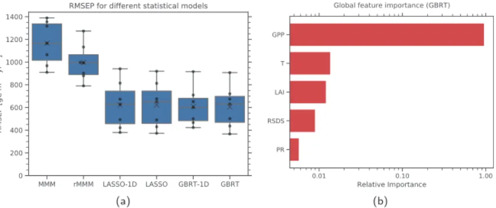
In terms of raw predictive power, the simple MMM is outperformed by every other model. Its prediction uncertainty expressed as mean RMSEP can be reduced by more than 48% by using other statistical models. However, this is not surprising: in contrast to the other statistical models, the simple RCP 8.5 MMM does not take further evidence in form of observations of the historical climate into account. Step 1 of our algorithm can reduce this mean RMSEP by 15% (rMMM) due to the single rescaling of the gridded climate model out-put with the global mean GPP constraint on the CO2fertilization effect. However, since there is a consider-ably large GPP range in the individual climate models themselves, this reduction is rather small for the gridded values. A far larger reduction of the RMSEP can be achieved by using the regression models LASSO‐1D, LASSO, GBRT‐1D and GBRT. All of them share similar RMSEP distributions, which can be explained as follows: The historical GPP is strongly (near linearly) correlated to the rescaled end‐of‐century GPP (with pattern correlation of R2 = 0.83 for the whole multimodel ensemble). Because of that, all Figure 4. (a) Boxplot of the root‐mean‐square error of prediction (RMSEP) distributions for six different statistical
models used to predict future absolute GPP (Step 2a) using a leave‐one‐model‐out cross‐validation approach. The distribution for each statistical model contains seven points (black dots, one for each climate model used as truth) and is represented in the following way: The lower and upper limit of the blue boxes correspond to the 25% and 75% quantiles, respectively. The central line in the box shows the median, the black“x” the mean of the distribution. The whiskers outside the box represent the range of the distribution. Compared to the CMIP5 multimodel mean (MMM) and its corresponding rescaled version (rMMM), the prediction uncertainty measured by the mean RMSEP is significantly reduced by up to 48% and 39%, respectively, when using other statistical models. Moreover, the nonlinear GBRT models can slightly reduce the mean RMSEP compared to the linear LASSO models by about 2% for GBRT‐1D (using historical GPP as single predictor) and 3% for the full GBRT model (using all predictors). (b) Relative global feature importance for the different features used in the GBRT model to predict future absolute GPP (Step 2a). The red bars correspond to positive Pearson correlation coefficients between all predictors and the target variable. Due to its strong positive linear relationship with the future GPP, the historical GPP is by far the most important predictor in the model. A local feature importance map (using LIME) is not shown here because GPP is the dominant predictor for all grid cells.
regression models are able to considerably reduce the RMSEPs compared to the MMM and rMMM. This also shows that the GBRT models successfully learned the linear connection between past and future GPP. Moreover, the nonlinear GBRT models can slightly reduce the mean RMSEP even further compared to the linear LASSO models by about 2% for GBRT‐1D and 3% for the full GBRT model. This leads to the conclusion that in addition to the strong linear relationship between past and future GPP, there are small nonlinear relations between the predictors and the target variable that can be used to further reduce the RMSEP. Since the full GBRT model with access to all predictors shows the minimal mean RMSEP, we argue that it is beneficial for our approach to use the multivariate nonlinear GBRT model instead of a linear model because only the GBRT algorithm is able to make use of all features and exploit more complex relationships. The influence of the different predictors can be further analyzed by evaluating the global feature importance by using the whole training data set and the already trained model. This is shown in Figure 4b. The past GPP with its strong positive linear correlation to future GPP is the most relevant predictor of the trained model with a relative importance of approximately 95%. All other features show values of less than 2%. The global feature importance determines the expected impact of a feature in predictions of the target variable. In our GBRT model the prediction input data of historical GPP mainly determines the machine learning model's prediction of the future GPP in the RCP 8.5 scenario at the end of the 21st century. However, we emphasize that this is only valid for our specific setup (i.e., which variables are used, which algorithm is used, which climate models are considered, etc.). For another problem setup, the global feature importance could change significantly. Since the historical GPP is the most important predictor for all grid cells, we do not show the plot of the local feature importance using LIME. We can get further insights into our GBRT model by ana-lyzing the residuals of the prediction using an independent test data set. The resulting plots show that the algorithm is not overfitting the training data and that the prediction errors on the whole are approximately unbiased (see Figure S2a).
3.2.2. Observation‐Based GBRT Prediction of Absolute GPP
In this section, we use the different statistical models to predict absolute GPP at the end of the 21st century. For this, we feed observation‐based data (see Table 1) into the regression models GBRT, GBRT‐1D, LASSO, and LASSO‐1D.
The result of Step 1 on the gridded data is illustrated in Figure 5a, which shows the ratio between rMMM and MMM. This ratio is almost constant over the whole globe, which is not surprising due to the global nature of the rescaling (see Equation 2). The use of the global emergent constraint predicts a slightly lower GPP increase over the 21st century (39%) than the unweighted CMIP5 ensemble mean (43%). The corresponding ratio 39 % /43 % ≈ 0.91 is approximately equal to the mean value of rMMM/MMM (0.92). Consequently, the global estimate of rMMM gives a lower GPP at the end of the century (179 Gt C yr−1) as MMM (198 Gt C yr−1), which can be interpreted as a correction of the ESMs' overestimation of future GPP to changes in the atmospheric CO2concentration.
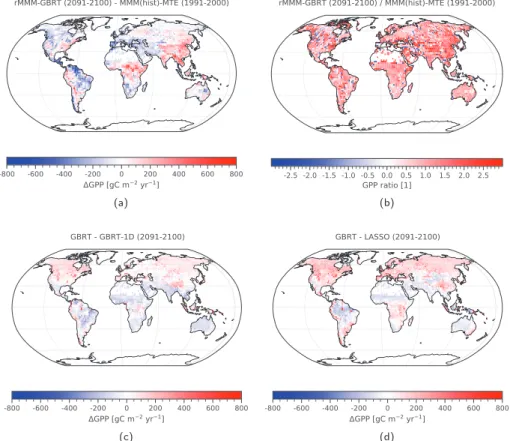
The spatial result of our GBRT model in Step 2a can be visualized by comparing rMMM and the output of the GBRT model. Figure 5b shows the bias of the rescaled CMIP5 RCP 8.5 multimodel mean compared to our GBRT predicted GPP at the end of the 21st century (2091–2100), while Figure 5c shows the bias of the his-torical CMIP5 multimodel mean compared to the observational FLUXNET‐MTE product (Jung et al., 2011) averaged for the period 1991–2000. As reported by Anav et al. (2013), the historical CMIP5 ensemble mean overestimates GPP in most regions, leading to a global mean of 138 Gt C yr−1, which is larger than the 123 Gt C yr−1estimate for the FLUXNET‐MTE product. Regions where GPP is largely overestimated are the western parts of South America, central and southern Africa, and East Asia. On the contrary, GPP is underestimated in small areas of Central America and northern parts of South America. The bias patterns in Figures 5b and 5c are very similar (pattern correlation of R2= 0.88), which means that the GBRT algo-rithm detects regional biases in the historical simulation and corrects them in its future predictions. This is also illustrated in Figure 6b, in which many values are close to 1, while only a few negative values exist. However, we emphasize that our approach is only tofirst order a bias correction (i.e., subtracting the histor-ical bias from the RCP 8.5 multimodel mean). There are clear differences between Figures 5b and 5c, which are also illustrated in Figures 6a and 6b. A simple bias correction would only show constant values for the whole globe, whereas our approach applies different corrections (in sign and magnitude) for different regions. On the global domain, our approach predicts a GPP at the end of the century of 169 Gt C yr−1,
which is consistent with the global constraint from Step 1 (171 ± 12 Gt C yr−1). In summary, our approach first corrects the CMIP5 models response to CO2(Step 1) and second corrects the historical bias of the ESMs relative to observations (Step 2a).
Further illustrations of these results including the uncertainties can be found in Figures S3–S5. Analogous to the results from the leave‐one‐model‐out cross‐validation approach, the uncertainties on grid cell level are significantly reduced for the GBRT prediction compared to the multimodel mean results. These errors con-sider all three sources of uncertainty that we presented in section 2.3 (error in the GBRT model, error in the rescaling and error in the observational‐driven products). In contrast to that, the error derived from the leave‐one‐model‐out cross‐validation approach illustrated in Figure 4a only shows the error in the statis-tical models themselves. We note that local relative errors can be very large (especially in regions with low absolute GPP) due to the uncertainty calculation method: Regardless of the absolute value, the error of each grid cell is at least 535 gC m−2yr−1(estimated SPE of the GBRT model using the RMSEP), which is added to the propagated errors of the observation‐driven data sets and the error derived resulting from the rescaling (Equation 2). The GBRT model error is the dominant source of uncertainty. Since the true covariance struc-ture of these globalfields is unknown, a global (or at least regional) aggregation of these uncertainties is not possible.
Figure 5. (a) Ratio of the rescaled CMIP5 ensemble mean of the absolute GPP at the end of the 21st century (2091–2100)
in the RCP 8.5 scenario using Equation 2 (rMMM) and its unweighted version (MMM). The plot shows an almost constant value over the whole globe with a mean of 0.92, which corresponds to the ratio of the constrained global mean GPP change over the 21st century (39%) and the CMIP5 ensemble mean global mean GPP change (43%) from Step 1. All values close to 0 for the data set in the denominator have been masked to avoid divisions by 0. (b) Bias between rMMM and our GBRT prediction of for the end of the 21st century. This corresponds to Step 2a of our approach. (c) Bias between the modeled GPP in the CMIP5 multimodel mean of the historical simulation and the FLUXNET MTE observation‐based estimate of GPP (Jung et al., 2011) averaged between 1991 and 2000. Over large swaths of the globe, the CMIP5 ensemble overestimates GPP (red color). Panels (b) and (c) show similar bias patterns (pattern correlation of
R2= 0.88). Thus, the GBRT prediction in Step 2a is able to correct the historical bias of the CMIP5 ensemble relative to the FLUXNET‐MTE product.
To further compare our GBRT approach to other statistical models, we also fed the observation‐driven data into the GBRT‐1D, LASSO, and LASSO‐1D models to get a constrained projection of the RCP 8.5 GPP. Figures 6c and 6d show the difference of the other models to the full GBRT approach. Both panels show values close to 0 for most of the globe (i.e., the difference between the GBRT and GBRT‐1D/LASSO is small), indicating that the bias‐correcting property of our approach is also present in the other regression models that use only the historical GPP as single predictors. Thus, we conclude that the bias correction of our GBRT model originates from the observation of the historical GPP, which is also supported by Figure 4b, which shows historical GPP as by far most important feature. On the contrary, second‐order corrections ori-ginate from the observations in the remaining predictors. These second‐order corrections are also visible as the nonzero values in Figures 6c and 6d. This indicates that using the nonlinear GBRT model with all fea-tures improves the final result. Moreover, the similar patterns in both panels demonstrate that the GBRT‐1D model emulates the strong linear relation of the historical GPP to future GPP and performs equally well as the linear models. The global estimates of 167 Gt C yr−1 (GBRT‐1D), 163 Gt C yr−1 (LASSO), and 162 Gt C yr−1(LASSO‐1D) are all consistent with the global constraint of 171 ± 12 Gt C yr−1.
3.3. Constraining Gridded Fractional GPP Change Projections (Step 2b)
In Step 2b, we constrain the gridded fractional GPP change over the 21st century (2100 vs. 2000) in the emission‐driven RCP 8.5 scenario (rescaled using Equation 2). This step is independent from Step 2a and only differs in the target variable (GPP change instead of absolute GPP). The remaining setup including the predictors, the GBRT model itself and the data sets are similar.
Figure 6. Difference (a) and ratio (b) of the both biases shown in Figures 5b and 5c. For panel (b), all values close to 0 for
the data set in the denominator have been masked to avoid divisions by 0. Both panels show that our approach is only tofirst‐order bias correction, in which case both plots would only show constant values. (c) Comparison of the GBRT versus GBRT‐1D projections of future GPP. This panel indicates a clear difference between the full GBRT using all predictors and the GBRT model using only historical GPP as single predictor. (d) Comparison of the GBRT versus LASSO projections of future GPP. This panel shows that there is a clear difference between using the nonlinear GBRT model and the linear LASSO model. The results of the LASSO‐1D model are not shown here because they are very similar to LASSO.
3.3.1. Prediction Error in a Leave‐One‐Model‐Out Cross‐Validation Approach and Feature Importance
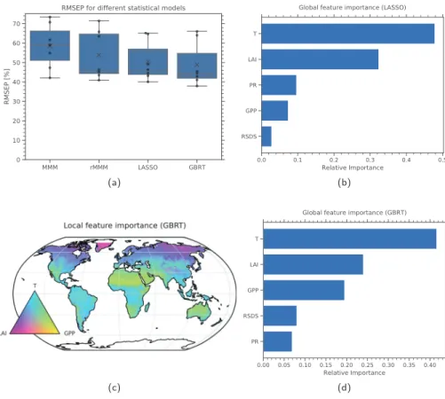
Figure 7a shows the RMSEP distributions for four different statistical models: the simple CMIP5 multimodel mean of the fractional GPP change (MMM), its rescaled version using Equation 2 (rMMM), a linear LASSO regression model and the GBRT model. Similar to Step 2a, the GBRT approach shows the smallest mean RMSEP values of all statistical models. Compared to MMM and rMMM the mean is reduced by 16% and 9%, respectively. Moreover, the nonlinear GBRT model also outperforms the linear LASSO model (mean reduced by 3%). In contrast to Step 2a, there is not a single predictor which heavily dominates the feature importance of the GBRT model. Thus, using single‐predictor models (GBRT‐1D and LASSO‐1D) is not necessary in Step 2b. Figures 7b and 7d show the global feature importance for the LASSO and GBRT model, respectively. Both models agree that the surface air temperature (T) and the leaf area index (LAI) are the two Figure 7. (a) Boxplot of the root‐mean‐square error of prediction (RMSEP) distributions for four different statistical
models used to predict the fractional GPP change over the 21st century (Step 2b) using the leave‐one‐model‐out cross‐ validation approach. The distribution for each statistical model contains seven points (black dots, one for each climate model used as truth) and is represented in the following way: The lower and upper limit of the blue boxes correspond to the 25% and 75% quantiles, respectively. The central line in the box shows the median, the black“x” the mean of the distribution. The whiskers outside the box represent the range of the distribution. The GBRT algorithm shows the minimal mean and median RMSEP. Compared to the CMIP5 multimodel mean (MMM) and its corresponding rescaled version (rMMM), the prediction uncertainty measured by the mean RMSEP of the GBRT model is reduced by more than 16% and 9%, respectively. Compared to the linear LASSO model, the RMSEP mean and median of the GBRT model are reduced by 3%. (b) Relative global feature importance for the different features used in the LASSO model to predict the fractional GPP change (Step 2b). The feature importance for the LASSO model is given by the (normalized) linear coefficients of the model. (c) Local feature importance for the GBRT model used to predict fractional GPP change (Step 2b) calculated using the LIME approach (Ribeiro et al., 2016) for the three dominant features T (surface air temperature), LAI (leaf area index), and GPP. The relative influence of these three features (ignoring all other features) is color coded according to the triangle in the lower left corner: The vertices correspond to a single dominating feature, whereas the center corresponds to an equal influence of all three features. Over large parts of the globe, T is the dominant feature. (d) Relative global feature importance for the different features used in the GBRT model to predict the fractional GPP change (Step 2b). The blue bars for the two global feature importance plots (b) and (d) correspond to negative Pearson correlation coefficients between all predictors and the target variable.
dominant predictors with a relative importance of more than 65%. The LASSO model shows a relative importance of less than 10% for each of the remaining features, while the GBRT model exhibits a considerably high relative importance for GPP with almost 20%. All predictors are negatively correlated to the target variable (as given by the sign of the linear Pearson correlation coefficient). That means cold areas with a small LAI in the historical climate show a larger GPP change over the 21st century and vice versa. Indeed, the fertilization effect is expected to be stronger in lower LAI regions. To get more detailed insights on this, observation‐driven data is fed into the GBRT model to obtain a constrained fractional GPP change over the 21st century.
3.3.2. Observation‐Based GBRT Prediction of Relative GPP
The global distribution of the fractional GPP change for the different statistical models is shown in Figure 8. All panels show a GPP increase over the 21st century in the RCP 8.5 scenario for almost all regions of the globe. Compared to the unweighted CMIP5 multimodel mean (MMM), its rescaled version (rMMM) shows a slightly lower GPP increase, which is consistent with the emergent constraint approach from Step 1 that shows a lower global mean GPP increase over the 21st century (39%) than the global CMIP5 ensemble mean (43%). This is also illustrated in Figure 9a, which shows an almost constant pattern over the whole globe with a mean of 0.91 that is consistent with the ratio 39 % /43 % ≈ 0.91. Similar to Step 2a, can be interpreted as a global correction of the ESMs' response of future GPP to changes in the atmospheric CO2concentration. All four patterns of Figure 8 show very similar geographical pattern. Obvious exceptions are the Sahara desert and the Arabian Peninsula, which show a noisy behavior for the multimodel means (MMM and rMMM) and a small GPP increase for the two regression models (LASSO and GBRT). This noise‐like pattern occurs due to numerical inconsistencies produced by very small values in the absolute historical and future GPP in the climate models in this region that are used to derive the fractional GPP change following Figure 8. Fractional GPP change over the 21st century (2100 vs. 2000) in the RCP 8.5 scenario for different statistical
models (Step 2b): (a) CMIP5 multimodel mean of the fractional GPP change (MMM), (b) rescaled CMIP5
multimodel mean using Equation 2 (rMMM), (c) linear LASSO model, and (d) GBRT model. The geographical patterns from the different statistical models are very similar showing a higher GPP increase in high latitudes and a lower GPP closer to the equator.
Equation 1. However, due to the small impact on the global mean GPP this region is negligible in our analysis. The fractional GPP change is not uniformly distributed over the globe. Instead, there is a pronounced latitudinal dependency in its geographical pattern: in high latitudes, the projected GPP change is larger than in regions closer to the equator. This effect is particularly strong for the Northern high latitudes and consistent with the results of Wenzel, Cox, et al. (2016), whofind an increased GPP change in northern high‐latitude ecosystems compared to the northern extratropics. A possible reason for this is the extension of the growing season in high latitudes caused by climate change connected to a “greening,” which has already been observed in the past climate through satellite measurements (Lucht et al., 2002; Myneni et al., 1997; Zhang et al., 2020) and associated with the increase in the CO2seasonal cycle amplitude (Forkel et al., 2016). This is consistent with the feature map in Figure 7c, which shows an increased relative importance of the LAI (a quantity directly related to the greening) in the high‐latitude regions with high GPP changes. On the contrary, in the tropical ecosystems the growing season already covers the whole year. Thus, a further climate change‐induced extension is not possible, leading to a smaller fractional GPP change in regions closer to the equator. For most parts of the remaining globe, the temperature (T) is the dominant predictor, with some areas in northern Africa, the Middle East, India and Australia showing an increased relative importance of the historical GPP. Overall, the negative correla-tion of the three most important features (T, LAI, and historical GPP) to the target variable is well reflected in the global pattern of the fractional GPP change: the high latitudes with lower T, lower LAI and lower Figure 9. (a) Ratio of the rescaled CMIP5 ensemble mean of the fractional GPP change over the 21st century using
Equation 2 (rMMM, see Figure 8b) and its unweighted version (MMM, see Figure 8b). The plot shows an almost constant value over the whole globe with a mean of 0.91, which corresponds to the ratio of the constrained global mean GPP change over the 21st century (39%) and the CMIP5 ensemble mean global mean GPP change (43%) from Step 1. All values close to 0 for the data set in the denominator have been masked to avoid divisions by 0. Absolute (b) and relative (c) differences between the fractional GPP change over the 21st century predicted by the GBRT model (see Figure 8d) and rMMM (see Figure 8b). For panel (c), all values close to 0 for the data set in the denominator have been masked to avoid divisions by 0. Both plots show a good agreement over large parts of the globe (corresponding to a value of 0). There are large absolute differences in the Sahara region and central Asia. The largest relative differences (except for the Sahara and Arabian Peninsula region) appear over South America, South Africa, the west coast of Africa, the Middle East, parts of Australia, and western parts of the United States.
historical GPP show higher GPP changes, whereas regions closer to the equator with higher T, higher LAI and higher historical GPP show smaller GPP changes. At this point we want to emphasize that it is not pos-sible to infer global or other large‐scale averages of the fractional GPP change from the geographical distri-butions in Figure 8 since division operations and averaging operations do not commute: in general, ∑i(xi/yi) ≠ (∑ixi)/(∑iyi). Thus, a direct comparison to other studies that give locally/globally aggregated results is not possible.
To get further insights in the GBRT algorithm, we compare it directly to the rescaled CMIP5 multimodel mean (rMMM), which is illustrated in Figures 9b and 9c. The mismatch between GBRT and rMMM can be interpreted as additional information that is added to the target variable by the observations in the pre-dictors in Step 2b. Overall, the absolute difference (Figure 9b) is small over the whole globe, indicating that the rMMM and GBRT agree in the general pattern of the fractional GPP change. The most striking deviation in this panel is again the Sahara and Arabian Peninsula region, which shows the already discussed large absolute differences. Apart from that, there is a large patch in central Asia that shows high negative differ-ences, that is, the GBRT model predicts a smaller GPP change in this area. The relative difference (Figure 9c) indicates many regions where the GBRT model predicts an increased GPP change compared to rMMM, in particular South America, South Africa, the west coast of Africa, the Middle East, parts of Australia and wes-tern parts of the United States. However, all these correspond to low absolute GPP changes. Figure S6 shows the corresponding gridded uncertainties for all four statistical models that also cover the uncertainty in the emergent constraint and the observational uncertainty (in contrast to Figure 7a, which only covers the uncertainty in the statistical models). Similar to Step 2a, the local standard errors are large, even for the GBRT model (that performs better than any other statistical model) which shows errors of at least 43.6% for every grid cell caused by the uncertainty in the statistical model itself. Figure S2b illustrates the residuals for the training and independent test data sets and shows that the GBRT model has symmetrical residuals and is not overfitting.
3.4. Comparison of the Absolute and Relative GBRT Prediction
In a last step, we use the FLUXNET‐MTE observational product to constrain the absolute GPP increase at the end of the 21st century (2091–2100) from the fractional GPP change given by the GBRT model in Step 2b. This can be directly compared to the output of Step 2a and serves as a sanity check between Steps 2a and 2b. As shown by Figure 10, both approaches show similar geographical patterns (pattern correlation
R2= 0.97). The difference between the two approaches is in the same order of magnitude as the difference between the different statistical models used in Step 2a (see Figures 6c and 6d) and considerably smaller than the difference between the GBRT and rMMM approaches (see Figure 5b). Moreover, the globally aggregated results (169 Gt C yr−1for Step 2a and 175 Gt C yr−1for Step 2b) are both compatible with the global value of 171 ± 12 Gt C yr−1given by the global emergent constraint in Step 1.
4. Summary and Discussion
In this paper, we developed a two‐step approach to constrain the projected GPP at the end of the 21st century (2091–2100) in the RCP 8.5 scenario. In the first step, we constrain the global mean GPP to 171 ± 12 Gt C yr−1using a published emergent constraint approach which we assume can also be applied to the global mean GPP at the end of the 21st century in the RCP 8.5 scenario (see discussion in section 2.1). This step corresponds to the correction of the ESM's biases in the response of future GPP to rising atmo-spheric CO2 concentration, which is the main source of uncertainty in future GPP projections (Arora et al., 2013; Haverd et al., 2020; Rogers et al., 2017). As already discussed in section 2.1, due to other than CO2fertilization drivers of the increase in the CO2seasonal cycle amplitude (Bastos et al., 2019; Forkel et al., 2016; Piao et al., 2018; Zhao et al., 2016) this emergent constraint is not undisputed and can be replaced with another emergent constraint in future studies. In the second step, a machine learning approach is used to further constrain the gridded GPP based on process‐based present‐day predictors. We consider two target variables:first (Step 2a) the gridded monthly climatologies of absolute GPP (2091–2100) and second (Step 2b) the gridded fractional GPP change over the 21st century (years 2091–2100 vs. years 1991–2000, see Equation 1). Both approaches give consistent results (see Figure 10). The latter quantity shows an increased GPP change in the high latitudes compared to regions closer to the equator, which might be attributed to an additional greening trend in the high latitudes as supported by the feature map in Figure 7c that shows the
LAI as dominant predictor in this region. However, in the absence of a robust physical mechanism this connection cannot be proven. For both target variables, the GBRT algorithm is superior to all other considered statistical models in terms of prediction uncertainty evaluated in a leave‐one‐model‐out cross‐ validation approach among different statistical models. Compared to the unweighted CMIP5 multimodel mean the mean prediction error is reduced by 48% (Step 2a) and 16% (Step 2b); compared to a linear LASSO regression model the mean prediction error is reduced by approximately 3% for both cases. However, local standard errors are still large for both target variables, even for the GBRT model. Due to the unknown covariance structure a global aggregation of these errors is not possible. Step 2a mainly corrects the bias of the simulated absolute historical GPP relative to observations (Anav et al., 2013). Consequently, the historical GPP is by far the most important predictor for future absolute GPP (regions with high GPP in the past are likely to have high GPP in the future and vice versa). However, as we have shown in Figure 6, the GBRT model expands this bias correction by taking more predictors than the historical GPP into account. A similar result is provided by Step 2b: Figures 9b and 9c show the impact of the additional predictors as difference between the CMIP5 multimodel mean and the GBRT predicted GPP change. In this case, the target variable (fractional GPP change) was already normalized with the historical GPP. Therefore, the temperature (second most important feature in Step 2a) is now the most important predictor instead of historical GPP (see Figure 7d). As shown in Figure 7c, the different features have also different dominant regional impacts; but again, since there is no distinct physical mechanism relating the predictors to the target variable this map needs further analysis and treated with care.
Our GBRT approach (Steps 2) is mathematically similar to MDER (Karpechko et al., 2013; Senftleben et al., 2019; Wenzel, Eyring, et al., 2016): we establish a relationship between process‐oriented, physically relevant diagnostics and future projections and then utilize this to predict today's observed conditions into Figure 10. (top row) Absolute future GPP at the end of the 21st century (2091–2100) calculated using (a) Step 2a and
(b) Step 2b. Both approaches give similar results, with global averages of (a) 169 Gt C yr−1and (b) 175 Gt C yr−1, which are both consistent with the global result of Step 1 (171 ± 12 Gt C yr−1). The pattern correlation between both approaches is R2= 0.97. (bottom row) Absolute (c) and relative (d) differences between panels (a) and (b).