Decadal trends in atmospheric organic aerosol :

Decadal trends in atmospheric organic aerosol:

Analysis of network data and method development

by

Kelsey Jane Boulanger

B.S. Civil and Environmental Engineering University of California, Berkeley (2012)

ARCHVES

OF TECHNOLOGY

DEC 0 U

2015

LIBRARIES

Submitted to the Department of Civil and Environmental Engineering

in partial fulfillment of the requirements for the degree of

MASTER OF SCIENCE IN CIVIL AND ENVIRONMENTAL ENGINEERING

at the

MASSACHUSETTS INSTITUTE OF TECHNOLOGY

September 2015

2015 Massachusetts Institute of Technology. All rights reserved.

A uthor...

Certified by...

Signature redacted

Department of Civil 2

Environmelal Engineering

August 20, 2015

...

Signature redacted

Jesse H. Kroll

Associate Professor of Civil, Enviro

ental, and Chemical Engineering

A ccepted by...

1/

Signature redacted

I _/

_I-i

Donald and Martha Harleman Professor of Civil and Environmental engineering Chair, Graduate Program Committee

...

Decadal trends in atmospheric organic aerosol:

Analysis of network data and method development

by

Kelsey Jane Boulanger

Submitted to the Department of Civil and Environmental Engineering on August 20, 2015 in partial fulfillment of the

requirements for the degree of Master of Science in Civil and Environmental Engineering

ABSTRACT

Organic aerosol (OA) makes up a substantial fraction of atmospheric particulate matter, yet its sources and controlling factors - and thus its impacts on climate and human health - are not well understood. Recently-developed analytical techniques have provided new insight into OA chemistry, but major uncertainty remains in how OA has changed over the past few decades. Characterizing long-term trends in OA would allow for better calibration of models that currently struggle to replicate ambient organic measurements as well as answer questions of how changes in OA relate to changes in emissions sources, anthropogenic-biogenic emissions interactions, altered chemistry, and more. This work represents a two-fold effort to better constrain our understanding of OA trends spatially, temporally, and chemically. First, trends in aerosol species concentrations over the past two decades are examined using existing data from the U.S. Interagency Monitoring of Protected Visual Environments (IMPROVE) network to provide insight into the long-term OA evolution across the rural U.S. Along with large decreases in total aerosol amounts (30-50%), OA is found to decrease at a fractional rate nearly equivalent to the decreases in three other major aerosol species: nitrate, sulfate, and elemental carbon. This suggests a link between the controlling factors of the different species, but explaining these observations is made challenging by the lack of chemical characterization of historic OA measurements that would help point to changing sources and chemistry. Thus, the second part of this work introduces a technique that enhances our ability to obtain important chemical information from small-volume environmental aerosol samples, such as filter extracts from remote regions like those monitored by the IMPROVE network, that were previously excluded from Aerodyne aerosol mass spectrometer (AMS) analysis due to the prohibitive volumes required for standard atomization. The Small Volume Nebulizer (SVN) nebulizes microliter-sized liquid samples, allowing for highly time- and mass-resolved chemical analysis of dissolved organic species on the AMS and providing valuable insight into the factors that control observed

OA trends. By examining historic trends in particulate matter loading and composition, and

expanding AMS coverage to include small-volume environmental samples, we can begin to answer the question of how and why OA has changed over the past few decades - and what that means for OA chemistry, the climate, and regional and global air quality.

Thesis Supervisor: Jesse H. Kroll

Acknowledgements

This project is based upon work supported by the National Science Foundation Graduate Research Fellowship under Grant No. 1122374, with additional funding from the National Oceanic and Atmospheric Administration Grant No. NA130AR4310072. For the work on the Small Volume Nebulizer, I would like to thank our collaborators Manjula Canagaratna, John Jayne, and Phillip Croteau from Aerodyne Research Inc as well as Jason Surratt and his research group for providing us withfilter extracts.

This work would be incomplete were it not for the incredible members of the Kroll research group. Anthony Carrasquillo, Kelly Daumit, James Hunter, Eben Cross, Chris Lim, Ellie Browne, Sean Kessler, Jon Franklin, David Hagan, Gabriel Issacman-VanWertz, and Rachel O'Brien: thank you all for your generosity of knowledge, advice, energy, and spirit. I will forever cherish memories of days spent in and out of lab with you all, exploring new cities for conferences, jumping rope in 5-degree-Fahrenheit weather, consuming excessive amounts of (non-alcoholic) butterbeer in Harry Potter World, teaching chemistry to eager high school students, fighting (non-literal and literal) fires in lab, and passing the torch on the SVN (which remains a boring acronym despite some of your best efforts to make it otherwise!). It's been an amazing three years with an absolutely stellar research group. You'll all be dearly missed.

I owe my sanity to my friends and family. In addition to the extended Parsons community, who

make this building a home and who are too numerous to name but are all amazing, I want to specifically thank Katie Dailey for our weekly Skype conversations; Andrea Gutierrez for internet article swapping; Erin Connor and Jenn Apell for girls' nights; Amy Lu and Ana Ebrahimi for being my pen pals; Kyle Delwiche, Joseph Abel, and Alex Konings for game nights; and Anthony Carrasquillo for our shared (questionable) consumption of pop culture. Many thanks to my amazing sister, Lauren, for philosophizing on our shared upbringing and subsequent views of the world, and to my incredible mom and dad, for loving, supporting, and cheering for me more than I can understand. And to my wonderful husband, David: marrying you was the best thing to come out of my experience at MIT. Thank you for everything you do to make our lives so fulfilling and enriching. (Also: official apologies to Jesse and Colette for all the time we wasted while we fell in love instead of working!) Each and every one of these people gave me the strength I needed to make it to MIT in the first place, to complete this degree, and to follow my passion into teaching. I'll never be able to thank you all enough.

Most of all, I want to thank my research advisor, Jesse Kroll. Not a single graph or statement of this thesis would have been possible without his tireless enthusiasm, generous encouragement, and patient understanding (often undeserved). Jesse, your mentorship and inspirational leadership are the main reasons I am sad to graduate. You are one of the kindest people I have ever met; if I could teach while working for you forever, I would without question. I will do my best to pay forward the grace you have shown me by extending similar compassion to all of my future students. Thank you so much for everything.

Contents

1. Introduction ... 11

2. Evidence for Decreasing Organic Aerosol Concentrations in the Rural United States Over the Last Q uarter-Century ... 19

2.1 R ationale ... 19

2.2 M ethod ... 20

2.2.1 IM PROV E N etwork ... 20

2.2.2 Data A cquisition...23

2.2.3 D ata A nalysis...24

2.3 R esults and D iscussion... 26

2.4 Conclusions... 36

3. Development of a nebulization technique for obtaining AMS spectra from small volum e liquid sam ples... 39

3.1 M otivation ... 39

3.2 M ethods... 40

3.2.1 Sm all Volum e N ebulizer...40

3.2.2 Standards and Sam ple Generation and Storage... 42

3.2.3 D ata Collection and Processing...43

3.3 R esults and D iscussion... 45

3.3.1 Technique Characterization...45

3.3.2 Com parison w ith Standard Atom ization ... 48

3.3.3 Determ ination of the Optim al Sam ple Solvent... 50

3.3.4 Testing Laboratory SOA ... 52

3.4 Conclusions... 56

4. Sum m ary ... 59

6. A ppendix... 69

6.1 A verage A erosol Pie Charts for Individual IM PROVE Sites ... 69

6.2 Com paring SVN Film s...78

List of Figures and Tables

FIGURES

Figure 1: IM PROVE Network Locations ... 21

Figure 2: Schem atic of the Im prove Sampler ... 23

Figure 3: Regional Average Composition and Total Loading of Particulate Matter for the United States in 1990 and 20 10 ... 33

Figure 4: Average Regional Trends in Aerosol Species Relative to their 1990 Values... 34

Figure 5: Investigating Biomass Burning Effects... 35

Figure 6: Investigating Weekday and Weekend Effects... 35

Figure 7: Investigating the Relationship Between Organic Mass and Sulfate... 36

Figure 8: Sm all Volum e N ebulizer Set Up ... 42

Figure 9: Filter Sam ple Extraction M ethod ... 43

Figure 10: Comparing the Mass Observed in the AMS to both the Droplet Size and Nebulized M a ss ... 4 9 Figure 11: Comparing the SVN Technique to the TSI Atomizer ... 47

Figure 12: Particle Size and Signal Produced for Different Solvents... 51

Figure 13: Comparing Online AMS with Offline SVN Measurements for Different Solvents ... 55

Figure 14: Comparing Online ACSM with Offline SVN-AMS Measurements for an SOA E x p erim en t... 5 6

TABLES

Table 2: Ammonium-to-Nitrate and Ammonium-to-Sulfate Ratios for the Solution, the TSI Atomizer, and the SVN Nebulization Technique. ... 49

APPENDIX

Appendix 1: IMPROVE Site Abbreviations... 69

Appendix 2: Sites Locations in the Western United States ... 70

Appendix 3: Average Aerosol Pie Charts for the Western United States... 71

Appendix 4: Site Locations in the Mid-United States ... 72

Appendix 5: Average Aerosol Pie Charts for the Mid-United States... 74

Appendix 6: Sites Locations in the Eastern United States... 75

Appendix 7: Average Aerosol Pie Charts for the Eastern United States... 76

Appendix 8: Additional IMPROVE Sites Not Included in the Three Regions ... 77

A ppendix 9: Polyester Film Test R esults... 78

Appendix 10: FEP Film Test Results ... 79

Appendix 11: Kapton Polimide Film Test Results ... 80

A ppendix 12: Teflon Film Test Results... 81

1. Introduction

Atmospheric particulate matter ("aerosol") can have a profound influence on human

health, global climate, and air quality. Aerosols affect cloud formation and light scattering in the

atmosphere, which in turn can influence the radiative balance of the atmosphere and have

important impacts on climate (Yu et al., 2006; IPCC, 2013). Ambient aerosol exposure has been

linked to daily mortality, and respiratory and cardiovascular system damage (Schwartz et al.,

1996; Harrison and Yin, 2000; Davidson et al., 2005; Arden Pope III and Dockery, 2006).

Particle reactions can produce more toxic compounds with potentially mutagenic and

carcinogenic effects (Finlayson-Pitts and Pitts, 1997). We need to understand aerosol formation, composition, and aging processes in order to address their health and environmental impacts, but

our knowledge of these aerosol characteristics is currently limited. One research avenue that will

help us address some of these unknowns is developing an understanding of historical aerosol

trends. This will allow us to better identify aerosol sources, characterize aerosol responses to

regulations and other changing factors, and calibrate models for investigating the factors that

contrpl aerosol. There are two main strategies for characterizing historical trends: analyzing

existing data for trends, and expanding the dataset by measuring the chemical composition of

existing samples. The first strategy is addressed in Chapter 2 with the analysis of aerosol data

from rural parts of the United States, and the second strategy requires method development that

is characterized in Chapter 3. The rest of this introduction will provide the background and

motivation for this two-fold approach to characterizing historical trends in aerosol.

As awareness of the dangers of poor air quality spread in the first half of the twentieth

effects of air pollution. The original Air Pollution Control Act of 1955 provided support for

research on air pollution but contained no regulatory actions; a series of acts followed that

strengthened the fight against air pollution by providing more funding, setting emissions

standards, and establishing regulatory bodies to enforce the changes (US EPA, 2015). The Clean

Air Act of 1963 was the first act to allocate funding for research into methods for monitoring and

controlling air pollution. The Motor Vehicle Air Pollution Control Act (1965) set up reductions

for hydrocarbons and carbon monoxide, which was followed by major amendments in 1970 that

expanded regulations to include both mobile and stationary sources. These amendments also

established the U.S. Environmental Protection Agency (EPA) and required it to enact National Ambient Air Quality Standards (NAAQS) for states to meet via individualized implementation

plans. The NAAQS dealt with the six criteria air pollutants, including sulfur dioxide, nitrogen

dioxide, and particulate matter. Efforts were expanded further with the 1990 amendments, which addressed a range of pertinent and emerging issues including smog, motor vehicle emissions,

acid rain, ozone depletion, and toxic air pollution. New emissions standards were implemented

for motor vehicles built after 1995. In 1997, the EPA tightened ozone and particulate matter

NAAQS. Each of these acts and amendments, which represent only a small selection of those

implemented during this period, helped establish stricter guidelines and controls on emissions and subsequently led to the reduction of many different air pollutants.

As a response to the various legislative acts, many national and state agencies were established to monitor the atmospheric concentrations of pollutants. The Clean Air Act required

each state to develop its own network of air monitoring stations, collectively titled the State and Local Air Monitoring Stations (SLAMS). Within this network is the National Air Monitoring Stations (NAMS), a subset of sites with more stringent requirements for equipment, quality

assurance, and reporting. These locations cover a range of locations, but are typically located in

urban regions where air quality monitoring is important for understanding health impacts on

daily life. Other urban sites are monitored by the Photochemical Assessment Monitoring Station

(PAMS), which measures ozone precursors, and the Speciation Trends Network (STN), which

monitors particulate matter at urban sites and was established by regulation in 1999 to support

attainment of the NAAAQS (CSU, 2010; IMPROVE, 2012). Conversely, where other agencies

monitor urban regions, the Interagency Monitoring of Protected Visual Environments

(IMPROVE) provides a picture of how air quality is changing at rural locations across the U.S.

IMPROVE was introduced in 1987 to help implement the Clean Air Act legislation by

identifying pollutants and sources causing impaired visibility in Class I areas (Joseph et al.,

1987; IMPROVE, 2012). Together, the large collection of monitoring networks run by both state

and government agencies provides a wealth of information about long-term changes in air

quality.

We can use the network data to look at how certain aerosol components that are better

understood have changed across the United States over the past few decades. Combining data

from a range of networks, the US EPA (2014) has found that particulate matter (PM) has

decreased nationally over the past few decades; these results are consistent with other studies on

fine PM (Blanchard et al., 2013; Murphy et al., 2011). Urban concentrations of sulfur dioxide

(SO2) and nitrogen dioxide (NO2) (precursors to sulfate and nitrate particulate matter) are well

characterized and have been steadily decreasing: the national average concentration of SO2

decreased by 75% and NO2 decreased by 45% over the past twenty years (US EPA, 2014).

IMPROVE data is particularly valuable for trend analysis because data has been collected for

IMPROVE sites, sulfate concentrations were shown to have decreased over the past twenty years of sampling (Malm et al., 2002; Hand et al., 2012). Decreases have also been observed in light

absorbing (EC) carbon concentrations (Murphy et al., 2011; Chen et al., 2012; Blanchard et al.,

2013) and total carbon (OC + EC) concentrations (Hand et al. 2013). Most of the decreases have

been linked to regulations controlling anthropogenic emissions (Murphy et al., 2011; Hand et al., 2012; Blanchard et al., 2013; Blanchard et al., 2015).

While these networks have provided valuable information on the trends in some aerosol components, many uncertainties persist in our characterization of aerosol due to historic and current limitations in instrumentation, source tracking, and chemical speciation of aerosol. One particularly influential source of uncertainty is the organic aerosol (OA) component of

particulate matter, which accounts for approximately 50% of total aerosol mass but remains poorly constrained in terms of chemical composition and knowledge of sources (Malm et al, 1994; Zhang et al., 2007; Jimenez et al., 2009). OA is characterized as either primary, having been emitted in the particulate form directly from a source, or secondary, which forms from the

oxidation of gas phase species and the subsequent condensation of lower volatility products

(Chung & Seinfeld, 2002; Tsigaridis & Kanakidou, 2007). In both forms, but especially secondary OA (SOA), OA presents a challenging task for characterization: identified organic species number in the thousands (Goldstein and Galbally, 2007), there are many complex reaction pathways and products often with non-linear behavior (Tsigaridis & Kanakidou, 2007), efforts to replicate environmental oxidation levels often fall short in the laboratory (Qi et al., 2010; Donahue et al., 2012), and models struggle to represent significant sources of OA that are likely secondary processes (Heald et al., 2005). Similarly, OA sources are not well understood because there are a wide variety and number of sources, volatile organic compounds (VOCs) can

be difficult to measure, SOA yields are not always well known for different VOCs, and reporting

of emissions inventories is subject to many uncertainties in measurement techniques, emission rates, chemical speciation, and more (Kanakidou et al., 2005). Although monitoring networks

provide valuable bulk speciation information, they are unable to distinguish the degree of

oxidation in their organic carbon measurements, which has been shown to be a good metric for characterizing OA (Kroll et al., 2011).

Fortunately, recently developed analytical techniques have provided new insight into OA composition where previously our understanding was extremely limited. One such instrument that is critical for the work in this thesis is the Aerodyne aerosol mass spectrometer (AMS),

which measures non-refractory sub-micron aerosol loading and chemical composition via flash vaporization of the particles with subsequent electron impact ionization of the vapor (Jayne et al., 2000; Allan et al., 2003; Jimenez et al., 2003; Drewnick et al., 2005). The AMS has been used in laboratories and field campaigns since its introduction in 2000 and has helped answer many questions about the chemical composition and loading of aerosol around the globe (e.g. Canagaratna et al., 2007; Zhang et al., 2007; Jimenez et al., 2009). Analytical instruments like the AMS have greatly expanded our ability to measure and chemically characterize OA both in laboratory studies and in-situ field campaigns.

However, there still remains a lack of historical information of OA due to the relatively recent introduction of these analytical techniques. The uncertainty in historical OA measurements has been particularly challenging for constraining model predictions. Global chemical transport models struggle to accurately represent total OA concentrations in the atmosphere (Bey et al., 2001; Kanakidou et al., 2005), and under-predict OA concentrations by factors up to 10-100 in the free troposphere, likely missing a source of secondary organic aerosol

(Heald et al., 2005). We do not have a good understanding of how OA has changed over the past

few decades. If we are to better predict OA effects on important environmental issues, we need to develop a historic OA record to provide insight into OA changes in the US, and how these

changes relate to emissions regulations, changing vehicle fleets, large biomass burning events, and other activities that affect organic concentrations so we can better model the processes that control OA (Kanakidou et al., 2005). One way to develop this historic record is by examining existing data from the national networks and comparing the aerosol trends with other changing variables like the emissions changes due to the previously mentioned policies. Correlating OA with anthropogenic activities will help us identify how much OA can be attributed to these activities, and therefore how much particulate OA we can control with regulation. With better insight into the controlling OA factors, we can better predict what future changes will improve air quality further as well as help constrain projections of future air quality and climate conditions.

A second way to develop this historic record is by analyzing stored historic samples using

modem measurement techniques. Many of the monitoring networks have collected aerosol samples on filters or in liquid samples to be analyzed at a later date or separate location, including the STN and IMPROVE (Coutant & Stetzer, 2001; IMPROVE, 2012). These networks provide valuable spatial and temporal coverage of aerosol information, as well as an opportunity for further analysis of archived samples and more extensive analysis of modem samples using instruments that are too costly or unwieldy to transport for in-situ analysis. However, in order for these archived samples to be analyzed using modem techniques, they must be converted into useable forms like liquid filter extracts. For the AMS, atomizers are frequently used to convert liquid samples into aerosol for analysis. This technique limits our ability to analyze

small-volume samples because standard atomization requires tens of milliliters of liquid. To expand the

dataset to include AMS characterization of archived samples, it is necessary to develop a method

that will allow for the extraction and analysis of microliter-sized liquid solutions on the AMS.

These two approaches for developing an understanding of historic trends in aerosol

-analyzing existing data for trends and developing a technique for modem analysis of historic

samples - are addressed in this thesis. The main research objectives that guided our analysis with respect to these two approaches are to:

(1) Analyze how aerosol amount and composition has changed in the rural United States

over the past twenty years; and

(2) Develop a technique that will allow us to analyze small-volume liquid samples on the

AMS and gain valuable insight into their chemical composition.

In Chapter 2, we tackle the first objective by analyzing historical trends in aerosol at rural sites

across the United States using data from the Interagency Monitoring of Protected Visual

Environments (IMPROVE) network. We present evidence of large decreases in total aerosol

concentrations with simultaneously small changes in aerosol composition over this time period, and discuss potential explanations for these trends. The work in Chapter 2 provides motivation

for the work in the following chapter, where we develop a nebulization technique that will allow

us to analyze more extensive data both spatially and temporally using the AMS. Chapter 3

introduces the Small Volume Nebulizer (SVN), including a description and characterization of

the technique as well as preliminary results from field and laboratory SOA studies. The future of

the technique is discussed in terms of both suggested improvements as well as a range of

implications and questions raised by the observed trends in rural aerosol, and how the SVN can provide valuable new information to the discussion of organic aerosol.

2. Evidence for Decreasing Organic Aerosol

Concentrations in the Rural United States

Over the Last Quarter-Century

2.1 Rationale

As discussed in Chapter 1, our understanding of organic aerosol (OA) sources and

controlling factors, and thus its impacts on climate forcing and human health, is hindered by

uncertainties in how OA has changed over the past few decades. The analysis presented in this chapter seeks to resolve some of that uncertainty by using existing aerosol data from the U.S. Interagency Monitoring of Protected Visual Environments (IMPROVE) Network to examine recent trends in aerosol species concentrations. One of the many monitoring networks in the

U.S., IMPROVE offers the opportunity to examine rural locations where biogenic emissions

contribute significantly to the makeup and where we can consider how changes in anthropogenic

emissions of sulfate, nitrate, and elemental carbon are related to changes in both anthropogenic

and biogenic sources of organics. While the accuracy and specificity of the US networks' previous OA measurements are limited by the technology used to obtain them, we can still develop a general understanding of how organics have evolved in the atmosphere over the past twenty years from this data.

IMPROVE data is particularly valuable for trend analysis because data has been collected for over twenty years at spatially distributed sites with consistent sampling methods. An analysis of the existing data on OA in the US, combined with a comparison to the better-constrained

measurements of sulfates and nitrates, will provide an introductory understanding of the ratio of

characterization of atmospheric organics motivates and informs the subsequent development of a nebulization technique (Chapter 3) for obtaining measurements of archived filter samples using modem aerosol analytical techniques, which ultimately will provide us with a new understanding of the global temporal evolution of organic aerosols.

This chapter focuses on IMPROVE data available on the Visibility Information Exchange Web System (VIEWS) website. Using IGOR Pro, raw data is analyzed for twenty-five different locations from 1990 to 2010. Changes in OA are characterized both on an absolute scale and relative to other key atmospheric constituents, including sulfate, nitrate, and ammonium. The observations are used to discuss potential controlling factors for OA trends and are interpreted in terms of historic changes to a number of factors that may affect relative and absolute loadings: emissions of primary organic aerosol (POA), changes in emissions of precursors to both secondary organic aerosol (SOA) and secondary inorganic aerosol, and other factors that may affect aerosol formation (e.g., NOx levels and aerosol acidity). By examining trends in particulate matter loading and composition, we can begin to answer the question of how OA has changed over the past few decades and what that says about the factors rontroling OA concentrations.

2.2

Method

2.2.1 IMPROVE Network

This project uses data from the US rural-based IMPROVE network. The network was started in 1985 to support the 1977 Clean Air Act, and was intended to monitor visibility impairment in Class I areas (mainly, national parks > 6000 acres, wilderness areas and national memorial parks > 5000 acres). It is run by a steering committee of representatives from eight

agencies, including the EPA, the National Park Service (NPS), and the USDA Forest Service

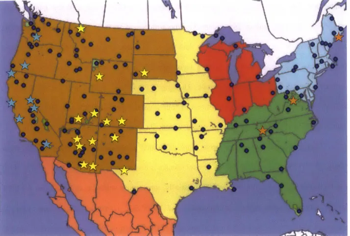
(USFS). Figure 1 shows the locations of the more than 200 IMPROVE measurement sites; the 25

sites used in this study are marked with stars and colored by their grouping into western (blue), mid-US (yellow), and eastern (orange) regions.

Figure 1: All IMPROVE Network locations. Sites included in this study are marked with a star, where the color of the star represents the division made in this work to represent the Western states (blue), mid-US states (yellow), and Eastern states (orange). Figure adapted from the IMPROVE website.

IMPROVE samples were collected bi-weekly every Wednesday and Saturday in 24-hour

increments (local time midnight to midnight). The sampling process is presented in detail by the

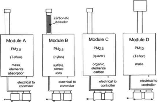
Figure 2, samplers consist of four modules: a primary Teflon filter for fine particulates and PM10 analyzed using gravimetric Particle Induced X-Ray Emission/Proton Elastic Scattering

Analysis (PIXE/PESA) X-Ray Fluorescence (XRF) absorption, a nylon filter with preceding

denuder for nitrates and sulfates analyzed using ion chromatography (IC), and tandem quartz filters for carbon fraction measurements analyzed using Thermal Optical Reflectance (TOR) combustion. The Teflon filters were analyzed in Davis, California with a validated data recovery rate >95%. Up to one-half to three-quarters of the nitrates and organics volatize during sampling and thus measurement values may be less than the actual mass. The nylon filters were analyzed at Research Triangle Institute or Global GeoChemical; nitrate concentration represents only particulate nitrate and not gaseous nitrate. The quartz filters were analyzed at Desert Research Institute, calculating carbon concentrations in four organic fractions (OC) and three elemental fractions (EC), which are used in this report as summed OC and EC values.

Certain compounds in this project are calculated as composite variables derived from measured variables. Determination of aerosol species is discussed in detail by Malm et al. (1994) and University of California Davis (1995). Briefly, ammonium sulfate is calculated as 4.125*S for non-null particulate sulfur concentrations and 1.375*SO4 otherwise. Ammonium nitrate is calculated as 1.29*NO3. Sea salt is calculated as 1.8*ClF for non-null chloride concentrations and 1.8*Cl otherwise. Total organic carbon is the sum of the organic carbon fractions and total

Module A Module B Module C Module D

PW6 ". PlMto

I

e0Ca ARM- * X*O&l 00iaC00

Figure 2: Schematic of the IMPROVE sampler showing the four modules with separate inlets and pumps. (From

http://vista.cira.colostate.edu/improve/Overview/IMPROVEProgramfiles/v3_document.html)

2.2.2 Data Acquisition

IMPROVE data was downloaded from the VIEWS Data Wizard public archive

(http://views.cira.colostate.edu/fed/DataWizard/Default.aspx), an online integrated database

compiling data from over a dozen monitoring networks and campaigns. This project uses a

subset of data from the IMPROVE network. Download setting selections made on the Data

Wizard are provided in Table 1.

The twenty-five sites included in this study were selected because they have the oldest

and longest-running data sets in the IMPROVE aerosol network, monitored bi-weekly from 1988

to 2011. A few additional sites were sampled during this time period but were not included

had inconsistent monitoring years (Everglades, FL), or they were from an urban area (Washington D.C.).

Table 1: Data Wizard selections for IMPROVE data used in this study.

PULL DOWN TAB SELECTION

Reports Raw Data

Datasets IMPROVE Aerosol

Sites Acadia National Park, ME; Badlands National Park, SD; Bandelier, National Monument, NM; Bliss State Park, CA; Bridger Wilderness, WY;

Bryce Canyon National Park, UT; Canyonlands National Park, UT; Chiricahua National Monument, AZ; Crater Lake National Park, OR; Glacier National Park, MT; Great Sand Dunes National Monument, CO; Great Smoky Mountains National Park, TN; Guadalupe Mountains National Park, TX; Indian Gardens, AZ; Mount Rainier National Park,

WA; Petrified Forest National Park, AZ; Pinnacles National Monument,

CA; Point Reyes National Seashore, CA; Redwood National Park, CA;

Saguaro National Monument, AZ; San Gorgonio Wilderness, CA; Shenandoah National Park, VA; Tonto National Monument, AZ; Weminuche Wilderness, CO; Yosemite National Park, CA

Parameters Ammonium Nitrate (Fine), Ammonium Sulfate (Fine), Elemental Total Carbon (Fine), Organic Total Carbon (Fine), PM 10 Mass (Total), Nitrate (Fine), Sulfate (Fine)

Dates "By Date Range" from 3/2/1988 to 10/30/2011

Fields Select: Dataset, Site, Date, Parameter, Data Value, Unit, Latitude, Longitude

Filters Select Aggregations: Non-Aggregated; Select Flags: (none)

Options Output Medium: Excel; Row Format: Standard; Content Options: Data & Metadata; String Quotes: None; Missing Values: -999; Date Format:

MM/DD/YYYY

2.2.3 Data Analysis

All the data was imported into and analyzed with IGOR Pro, scientific data analysis

software developed by WaveMetrics. Data from the downloaded text files was input into IGOR, and divided into folders based on location names. This allowed for easier data handling, as all compound waves had the same name under the different folders (ex: "OCf Value" contained

organic carbon measurements under each location folder). Organic carbon (OC) values were

multiplied by a factor of 1.8 to convert to organic mass (OM); this factor was chosen as a

reasonable approximation based on urban and rural values suggested by Turpin and Lim (2001)

and IMPROVE-specific values suggested by Malm and Hand (2007), but the selection of this factor does not affect the resulting trends in OA.

Functions were created to run each of these tasks: reformatting the date, filtering the concentration, removing major fire influence, averaging yearly values, averaging monthly values, and making ratios of average values. Date waves were reformatted to facilitate easy identification of month and year information for each measurement point. The months were

taken from the original waves via string identification, but the years were pulled from the original wave and turned into a new wave of only year values to address the software's issues

handling the transition from "99" to "00." Concentration waves were filtered to replace all negative concentrations, representing missing values, with NaNs (Not a Number). Excluding data from dates where fine mass was greater than 50 pg m- minimized the impact of fires on measurements, and particularly organic carbon values. Average values for each compound were

calculated monthly, seasonally and yearly/temporally. The month-averaged values combine

measurements for each month across all years, averaged to the number of days with real (concentration 0) measurements (i.e. days with missing concentrations were not included in the

averaging). Seasonal measurements were divided according to the following cutoffs: Dec/Jan/Feb for winter, Mar/Apr/May for spring, June/July/Aug for summer, and Sept/Oct/Nov

for autumn. The year-averaged values combine measurements for each separate year, averaged to the number of days with real measurements. Ratios of organic carbon to other species were calculated by dividing the average monthly or yearly values. Additional waves were created

(Months and Years) for use in plotting the average values. To compare aerosol loading in 1990 with loading in 2010, data was averaged over 1989-1991 and 2009-2011 respectively when data for those years was available. For a few sites with limited data, the averages were calculated from 1990-1991 and 2009-2010 data only. Finally, sites were grouped according to location for regional comparisons: Western, Mid-United States, and Eastern (general grouping provided in Figure 1; specific site names provided in Appendix 2, 4, and 6). We selected broad groupings based on their similar trends and out of necessity due to the limited number of sites with data for the entire period; Malm et al. (2004) suggest much more detailed regional classifications, which should be considered for shorter-term studies with a greater number of sites in the dataset.

2.3 Results and Discussion

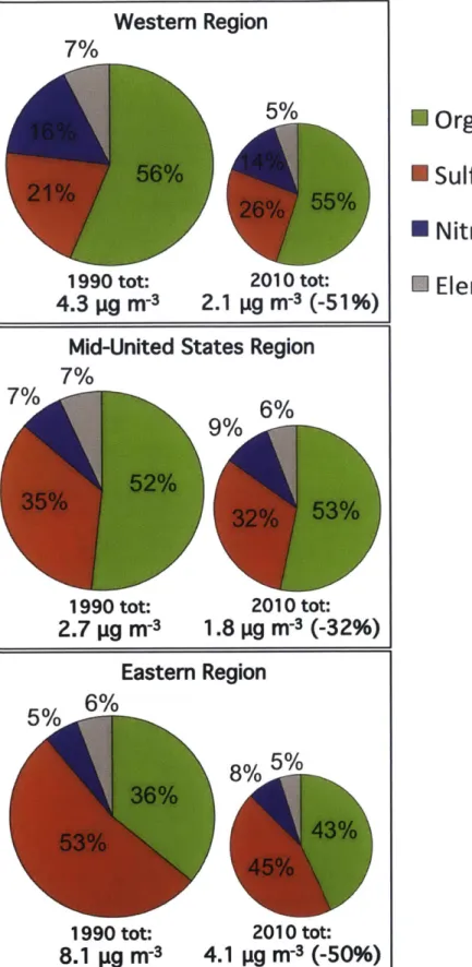
Total aerosol loading has dropped significantly (up to 60%) from 1990-2010 across the rural United States (Figure 3; Appendix 3, 5, and 7). The decrease is observed across all species considered here: sulfate, nitrate, elemental carbon (EC), and organic carbon (OC). The largest changes occur in the Western and Eastern regions, where respective average decreases are 49% and 51%. In the Midwest, the average decrease is only 31%. Despite the significant drop in total aerosol loading, the fractional composition has remained relatively unchanged: the pie charts in Figure 3 show how the total amount of each aerosol species has decreased much more strongly than any of the slight compositional changes. Notably, the organic fraction has stayed relatively constant, meaning total organic aerosol (OA) is decreasing despite no direct regulations on OA emissions other than potential reductions in primary OA (POA) that arise from controls on total particulate matter (PM) concentrations.

Figure 4 show the changes in average concentrations of each aerosol species relative to

their 1990 values and divided into the three major US regions. The Western sites have the closest

tracking of all four species, with the largest changes in EC and nitrate. This is likely due to the

Western sites being the closest to anthropogenic emissions and therefore reflecting the strong

emissions controls on EC and nitrate. Additionally, the Western sites start out with the largest

fraction of nitrate emissions relative to the other sites, and thus have the highest opportunity for

emissions controls to significantly impact nitrate concentrations. Conversely, the Eastern sites

see strong decreases in sulfate, OM, and EC with less change is nitrate. The strong decrease in

sulfate in the Eastern US is expected due to historically high sulfate concentrations and thus high

responses to anthropogenic sulfate emissions controls that have affected both stationary and

mobile sources, especially with regards to coal combustion. The Mid-US sites exhibit the

smallest decreases in aerosol species, which could perhaps be attributed to their initial total

aerosol loadings being smaller than the coastal sites (4.3 pg m3 in West, 8.1 in East, and 2.7 in

Mid-US; Figure 3) and therefore less responsive to emissions controls.

These results are consistent with other studies looking at aerosol composition and loading

during similar time periods. Over the period of 2000 to 2013, which is equivalent to the second

half of the period of data considered in our analysis, the US EPA (2014) measured an average

decrease of 39% in total particulate matter (PM) in the regions we have classified as Eastern,

20% in the Western region, and 14% in the mid-US region. Murphy et al. (2011) found 25%

decreases in rural EC and fine PM from 1990 to 2004 using IMPROVE data, and connected

these changes to emissions reductions. Hand et al. (2012) used rural IMPROVE data, urban

Chemical Speciation Network (CSN) data, and emissions reports from power plants to

concentrations and S02 emissions have been steadily decreasing from the early 1990s to 2010.

This suggests a linear relationship between anthropogenic S02 emissions and measured sulfate

concentrations, although some seasonal and regional trends were unexplainable with emissions

data and therefore indicate other contributing influences (Hand et al., 2012). Hand et al. (2013) looked at total carbon (TC = EC + OC) and found that over the same period considered here (1990 to 2010), there have been widespread decreases in rural TC with more seasonal variability

in the West as compared to the East. Other groups have also reported declines in EC in a variety of national networks (Chen et al., 2012; Blanchard et al., 2013). Blanchard et al. (2013) also report decreases in other important PM and gaseous species, including EC, organic matter, sulfate, nitrate, SO2, oxidized nitrogen species (NOy), carbon monoxide, and ozone, and link

these decreases primarily to emissions reductions; for fine PM, they suggest the decreases are a result of reductions in primary PM, including EC and some OM, as well as reductions of gas precursors known to form particles. Blanchard et al. (2015) looked at urban data in the Southern

region of the U.S. and attributed about half of the measured declines in OA to emissions

reductions for combustion processes, in eluding motor vehicle fossil-fuel use and biomass

burning, based on similar declines in EC and related gaseous species. Nguyen et al. (2015) find similar decreases in aerosol liquid water content and particulate OC, and link this to the hypothesis of water facilitating biogenic SOA formation.

There are a number of potential mechanisms that could explain the observed decrease in total OA. For those we were able to investigate, an explanation follows this list. Many of the

mechanisms will need to be considered from a modeling perspective or through greater data

collection in order to determine their impact on the observed trends. Changes in any of the following factors could be responsible for the OA observations:

- Biomass burning: Fires release OC into the atmosphere, so a decrease in fire activity

would result in lowered emissions of OC and thus lower OA concentrations.

- Meteorology: Biogenic emissions increase with temperature; a decline in temperatures

could lead to a decrease in OA precursor emissions. Rainfall represents a significant

aerosol deposition process, so increases in frequency and amount of rain could drive the

decreased concentration of OA. Another meteorological phenomenon that could

contribute to the observed OA decreases is relative humidity (RH): declines in RH would

lower the water content of inorganic aerosol, which could lead to lowered partitioning of

water-soluble gas-phase species into the particle phase.

- Land use: Biogenic emissions depend on vegetation type and amount, so changes in land

use such as deforestation or reforestation could alter total VOC emissions and the

composition of those emissions. Decreased VOCs concentrations, especially of species

with high SOA yields, could be responsible for the observed decrease in OA.

- Oxidant concentrations: Decreases in oxidants such as ozone and hydroxyl radicals

would decrease the oxidation of OC and therefore be expected to result in lower total OA.

- _{Primary OA emissions: If regulations that control particulate matter, like black carbon,}

have also led to decreasing emissions of primary OA, this could contribute to the

observed decline in measured OA.

- Secondary OA formation: Secondary OA (SOA) is formed from both anthropogenic

and biogenic emissions of VOCs. Decreases in SOA could be due to reduced VOC

emissions (lowered precursor concentrations would lead to reduced SOA formation), changes in aqueous aerosol content (it has been proposed that sulfate oxidation of VOCs

anthropogenic-biogenic chemistry. Reductions in anthropogenic emissions of species like

NOx, SOx could potentially alter the oxidation and formation of SOA, or indirect

reduction of anthropogenic VOCs in tandem with emissions regulations on other species

could decrease the precursors available for SOA formation.

Characterizing the extent to which any of these factors contribute to the observed trends

is beyond the scope of this work and would likely require extensive modeling. However, we can

begin to address the likelihood that some of these factors contributed to the trends by analyzing the existing data for trends in biomass burning markers, weekday/weekend effects, and sulfate

and organic measurements.

Changes in biomass burning could alter OA formation, but this is unlikely to explain our

observations due to the removal of large fire events from the data set. Additionally, Figure 5

shows that while potassium, a marker for biomass burning, and OA mass have similar trends, the

total fire acreage burned in the US has increased over this period and thus would be expected to

cause an increase in OA, not a decrease as observed. Snracklen et al- (2007) ao found an

increase in wildfire area burned between 1989 and 2004 with large inter-annual variability and a corresponding increased summer OC concentrations. Thus, although we cannot use our data to definitively rule out a change in biomass burning as a contributing factor to the observed changes in OA, it seems unlikely to be the reason OA has declined over this period.

To consider the influence of anthropogenic emissions, we separated changes in organic

mass (OM) and elemental carbon (EC) by their weekday and weekend effects. The weekday was

defined as Thursday + Friday and weekend was defined as Sunday + Monday based on work by Murphy et al. (2008). This division helps adjust for transport time for anthropogenic influences

to reach these remote regions and accommodates the shifted anthropogenic activity in national

parks relative to the normal urban classification of weekday-weekend. Because of a sampling

frequency shift in 2000 that provided more data for the weekday/weekend split, the trend is

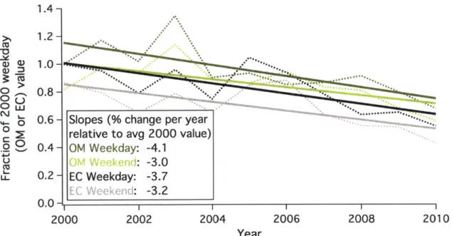
shown for post-2000 only. As Figure 6 shows, the fractional decrease is stronger for both EC and

OM on the weekdays than it is on the weekends. There is a larger weekly cycle for EC as

demonstrated by the larger gap in trend lines; the stronger weekly cycle in EC as compared with

OM is consistent with Murphy et al. (2008), who also found a pronounced weekly cycle in

nitrate similar to EC but no weekly cycle in sulfate. The similar behavior in EC and OM, as well

as nitrate, could indicate an anthropogenic mechanism controlling the observed decrease in OA.

Perhaps emissions reductions that controlled black carbon could have resulted in a similar,

unintentional reduction of organic particulates. Or perhaps there was a reduction in SOA due to

reductions in more chemically active particulate species like sulfate and nitrate, which have

similar trends as the EC due to shared anthropogenic sources. For example, it has been shown

that NO can drive SOA production from isoprene in urban regions; this mechanism could be

particularly influential in the Western region where NOx concentrations are the highest in the

U.S. and many sites are in close proximity to urban influences (Lin et al., 2013). Other groups

have suggested alternate mechanisms by which anthropogenic emissions can influence biogenic

SOA formation (Carlton et al., 2010; Hoyle et al., 2011; Schindelka et al., 2013). Regardless of

the mechanism, the presence of a weekday/weekend cycle in OA suggests that a significant

portion of the OA is either anthropogenically emitted directly or else influenced by

anthropogenic emissions via secondary pathways.

One potential secondary pathway is the sulfate-particulate water-organic mechanism.

partitioning of organics into aerosol (Carlton and Turpin, 2013); therefore, recent reductions in sulfate emissions might have driven the similar reduction in OA formation. Figure 7 shows how decreases in the total amount of sulfate and OM are correlated non-uniformly across the country. The correlations might be explainable by the Carlton et al. modeled mechanism, but the non-uniformity in this dataset could indicate a non-linear feedback of sulfate concentrations on OA. The recent reductions in sulfate emissions could be contributing to the reduction in OA formation either indirectly, through chemistry such as water partitioning, or directly, via simultaneous emissions reductions of organics along with directly regulated species. If emissions controls, which have reduced anthropogenic contributions to aerosol, have decreased OA loading as well, this would be a highly noteworthy unintended consequence of the regulations.

Western Region

7%

4.3 pg

M-

2.1 pg

M-

(-51%)

Organic

* Sulfate

* Nitrate

Elemental Carbon

Mid-United States Region

7%

2.7 pg

1.8 pg

(-32%)

Eastern Region

8.1 pg

M-

4.1 pg

M-

(-50%)

Figure 3: Average composition and total loading the rural United States.

1.4-2 1.1.4-2-

1.2-S 0.8 - __ ...

w-.6Slopes (% change per year

-o.6-relative to avg 1 990 value) -.. -..

C

.0 0.4- Nitrate: -2.4

U 0.2 Sulfate: -1.6 West Coast

EC: -2.7 1990 1995 2000 2005 2010 Year 1.4-2 1.1.4-2- 1.2-01) O ~ 0.8 -

-_---_---_---Slopes (% change per year

0 0.6 - _{relative to avg 1990 value)}

C . 0.4- Nitrate: +0.6 - M: -0.6 Mid-US u 0.2 Sulfate: -1.6 EC: -1.1 0.0- 1 1990 1995 2000 2005 2010 Year 1.4--2 1.2-1.0- -0 . -0) 0.8 - ___...__ ...

Slopes (% change per year

S0.6 - relative to avg 1990 value)

C

.2 0.4 Nitrate: -0.5

OM: -1.8 East Coast

2 0.2- Sulfate: -2.3

- EC: -2.5

0.0-1990 1995 2000 2005 2010

Year

Figure 4: Average trends in aerosol species relative to their 1990 values and divided by the three

US regions. The West and East coast regions had a 50% decrease in total aerosol between 1990

and 2010, whereas the Mid-US had a smaller average decrease at 30%. Organic aerosol mass decreased at an average of nearly 2% per year on the coasts and 0.6% per year in the mid-US.

2.0_ Slopes (% change per year relative to avg 1990 value)

Fire Acres: +2.1 > Potassium: -1.0 o 1.5- om: _-0.8 0.5 1990 1995 2000 2005 2010 Year

Figure 5: A comparison of organic mass and potassium with fire acres burned across the US to

investigate a potential biomass burning influence on OM trends. The similar percentage decrease in potassium and OA mass indicates a possible connection, but the increase in total fire acreage burned in US suggests biomass burning may not be responsible for organic decrease. (Fire data: National Interagency Coordination Center).

1.4-

1.2-(D -3.0

0>

0 L..

00.6 Slopes (% change per year

t2 relative to avg 2000 value)

O 0.4- OM Weekday: -4.1 U _-. S 0.2- EC Weekday: -3.7 EC Weekend: -3.2 2000 2002 2004 2006 2008 2010 Year

Figure 6: Average weekday (Th+F) and weekend (Su-IM) effects for all sites with data from post-2000 due to the sampling frequency shift in 2000.

0.0_ BRID

E West Coast W

Mid-US

o -0.5- East Coast SAGU YOSE

0 N _{TO iAC}

M

Total drop sulfate 1990-2010 (pg m3 )

Figure 6: A comparison between the total drop in organic mass with the total drop in sulfate over the 1990-2010 period. Regions are color-coded. Each of the regions has a unique slope associated with the correlated drop in species, suggesting non-uniform behavior across the country. Each point is identified by its site abbreviation (Appendix 1).

2.4 Conclusions

Examining existing data from the IMPROVE network allowed us to characterize the

historic trends in aerosol. Over the period 1990 to 2010, total aerosol loadings decreased by an

average of 30-50% across the rural United States. While the total loading decreased, the

fractional composition remained relatively constant. Notably, the organic aerosol (OA)

contribution decreased along with sulfate, nitrate, and elemental carbon (EC) species despite

emissions regulations that control only total particulate matter, not OA directly, and certainly not

secondary OA.

Potential factors controlling the observed decrease in OA are changes in biomass

burning, meteorology, land use, oxidant concentrations, primary OA (POA) emissions, and

related to the OA decrease due to the similar weekday-weekend trends in EC and OA as well as

the similar relationship between sulfate and OA declines. Modeling results have suggested that

biogenic SOA can be controlled up to 50% by anthropogenic emissions (Carlton et al. 2010);

therefore, it is possible that recent decreases in anthropogenic emissions could have resulted in a

decrease in measured SOA from both anthropogenic and biogenic emissions. Additionally, most

rural OA has been shown to be predominantly secondary (Brown et al., 2002; Zhang et al.,

2007), which suggests that the factors controlling OA trends are likely not associated with POA

emissions and instead related to factors that control SOA. If changes in anthropogenic emissions

were indeed one of the contributing factors, this would indicate that emissions controls have

been responsible for greater air pollution control than intended. However, better characterization

and explanation of the factors controlling OA trends will require extensive modeling that is

outside the scope of this study.

The work in this chapter provides motivation for the next chapter, where we develop an

instrument to analyze small filter extractions. IMPROVE data is constrained to basic, aggregate

measures of aerosol components. Analyzing this data allowed us to consider trends in total OA, but makes it difficult to understand precisely what is going on with the organic component: what

types of organic aerosols are decreasing? What is the cause of this decrease? Can we describe the

chemical composition changes due to changes in emissions or chemistry? These questions led us

to develop the Small Volume Nebulizer (SVN), which will allow for the future expansion of the

existing historical aerosol dataset by making it possible to collect detailed chemical composition

3. Development of a nebulization technique

for obtaining AMS spectra from small

volume liquid samples

3.1 Motivation

Atmospheric particulate matter (aerosol) is well understood to degrade air quality and

alter the radiative balance of the atmosphere, but direct characterization of aerosol effects is

difficult due to variances in aerosol reactions, composition, and spatial distribution. In particular, organic aerosol (OA) contributes significantly to this uncertainty. OA averages between 20 and

60% of aerosol mass worldwide (Zhang et al., 2007) and consists of thousands of different

organic compounds (Goldstein and Galbally, 2007). Despite its prevalence and importance, OA

remains difficult to capture in models. Model predictions of OA can be off by a factor of up to

100, significantly under-predicting the contribution due to secondary OA (Heald et al., 2005) and

hindered by our limited understanding of the complex OA chemistry and historical aerosol trends

with which we could calibrate the models.

Addressing the uncertainty in OA chemistry and composition, online aerosol mass

spectrometry (AMS) measurements provide important insights into the chemical composition of

particles. AMS deployment, however, is costly and restricted to a single location or field

campaign. Conversely, filter samples are routinely collected across the country and often around

the world, but analyses generally do not provide the same information (e.g., elemental ratios)

given by the AMS. Bridging the gap between techniques, and taking advantage of the valuable

insight provided by the AMS and the ease of filter collection, filter extracts offer an opportunity

In order to analyze filter extracts on the AMS, we need a technique that produces aerosol particles from small liquid samples. Traditional AMS measurements require atomization of

sample volumes on the order of milliliters, but filter extracts typically produce volumes on the order of microliters, especially if they must be concentrated. Here, we introduce the Small Volume Nebulizer (SVN): a nebulization technique that requires only a few microliters to characterize a sample. This technique allows us to gain valuable AMS information from small environmental samples and thus lends itself to a variety of useful and novel applications.

3.2 Methods

3.2.1 Small Volume Nebulizer

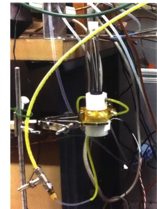
The Small Volume Nebulizer (SVN) coverts microliter-sized liquid samples into aerosol droplets, which allows for their introduction into the Aerodyne aerosol mass spectrometer

(AMS) for chemical analysis. The technique expands analysis of liquid samples to encompass

volumes too small for standard atomization. The SV-N is cased in PVC and is cylindrically shaped at 8cm tall with an outer diameter of 4.5cm and an inner diameter of 1.75cm where the tube connects at the top; Figure 8 shows a schematic of its structure. The primary nebulization mechanism works via a vibrating gold plate (Sonaer 2.4MHz nebulizer module with 24Au crystal) whose ultrasonic vibrations transmit through a reservoir of water and a 0.001" thick film of Kapton Polyimide, which is stretched over the reservoir of water, to nebulize liquid droplets placed in the center of the film. The vibrations are controlled via an on-off depressor switch. Clean house air input at 160 sccm through two side ports directs nebulized particles up the glass tube and into the HR-ToF-AMS. The glass tube was wrapped with Teflon tape around the

bottom to seal the airflow. The Kapton Polyimide film was wiped with a Kim Wipe as necessary

and rinsed clean with methanol before each series of runs. The glass tube was rinsed with

hexanes, dichloromethane, and methanol between uses.

Other films were tested, including 0.0005" polyester film and 0.002" thick Teflon RPTFE

film, but these were found unsuitable for the following respective reasons: too much organic

contamination and too thick to transmit enough ultrasonic vibrations to nebulize the droplet. An

additional film, 0.001" thick FEP film, was found to be suitable for use but was not selected

because the clear film color diminished droplet visibility and made it difficult to detect when

nebulization was complete. Results from the testing of these additional films are provided in

Appendix 9 through 12.

A sample droplet size of 8p.L was experimentally determined to maximize signal, and the

minimum observable sample concentration was determined to be ~0.15 g L-1 (Figure 10 in

Results). Droplets are placed on the film by lifting the glass tube and using a 10 p1 syringe to

inject the sample onto the center of the film. The glass tube is fitted back into place, we wait ten

seconds to allow any room air to flush out of the system, and then AMS collection is started. In

the original collection timing, droplets were nebulized once the "open" runs began and the entire

signal was measured in "open." In the subsequent collection timing, droplets were nebulized

once the "open" runs began but the signal was measured in both the "open" and "closed"

settings. MilliPore water droplets are used as the initial runs and between each sample as a blank

to verify that no particles remain on the film between samples. Each sample is run at least three