Multiple instance learning for sequence
data with across bag dependencies
Manel Zoghlami 1, 2, *, Sabeur Aridhi 3, Mondher Maddouri 4, Engelbert Mephu Nguifo 1
1 Clermont Auvergne University, CNRS, LIMOS, France
2 University of Tunis El Manar, Faculty of sciences of Tunis, LIPAH, Tunisia 3 University of Lorraine, CNRS, Inria, LORIA, France
4 University of Jeddah, College Of Business, KSA
Abstract
In Multiple Instance Learning (MIL) problem for sequence data, the learning data consist of a set of bags where each bag contains a set of instances/sequences. In some real world applications such as bioinformatics, comparing a random couple of sequences makes no sense. In fact, each instance may have structural and/or functional relations with instances of other bags. Thus, the classification task should take into account this across bag relation. In this work, we present two novel MIL approaches for sequence data classification named ABClass and ABSim. In ABClass, motifs are extracted from related instances and used in order to encode sequences. A discriminative classifier is then applied to compute a partial classification result for each set of related sequences. In ABSim, we use a similarity measure to discriminate the related instances and then build a scores matrix. For both approaches, an aggregation method is applied in order to generate the final classification result. We applied both approaches to solve the problem of bacterial Ionizing Radiation Resistance (IRR) prediction. The experimental results of the presented approaches are satisfactory.
Availability: Additional information about our datasets and our experiments can be found in the following link: http://homepages.loria.fr/SAridhi/software/MIL/
Keywords: sequence data classification, multiple instance learning, bacterial ionizing radiation resistance.
1. Introduction
In a traditional setting of machine learning, each instance is associated with a label. However, in Multiple Instance Learning (MIL), we have a set of bags where each bag contains multiple instances and it is the bag that carries a label. The labels of the instances that conform the bag could be unknown.
This work was originally proposed to solve the problem of bacterial Ionizing Radiation Resistance (IRR) prediction (Zoghlami et al. 2018; Aridhi et al. 2016). Each bacterium is represented by a set of protein sequences. This problem could be formalized as an MIL problem: bacteria represent the bags and protein sequences represent the instances. Each protein sequence may differ from a bacterium to another, e.g., each bag contains the protein named Endonuclease III, but it is expressed differently from one bag to another: these are called orthologous proteins (Fang et al. 2010). In order to learn the label of an unknown bacterium, comparing a random couple of sequences makes no sense, it is rather better to compare the protein sequences that have a functional relationship/dependency: the orthologous proteins. Hence, this work deals with the MIL problem that has the following three criteria:
1. The instances inside the bags are sequences: to deal with sequences, we have to deal with data representation. A widely used technique to represent MIL sequence data is to apply a preprocessing step which extracts features/motifs to represent the sequences (Sutskever et al. 2014; Saidi et al. 2010; Lesh et al. 1999). Other works keep data in their original format and use sequence comparison
techniques such as defining a distance function to measure the similarity between pairs of sequences (Aridhi et al. 2016; Xing et al. 2010; Saigo et al. 2004).
2. All the instances inside a bag contribute to define the bag’s label: the standard MIL assumption states that every positive bag contains at least one positive instance while in every negative bag all of the instances are negative. This is not guaranteed to hold in some domains so alternative assumptions are considered (Foulds and Frank 2010). Particulary, the standard assumption is not suitable for the above bacterial IRR prediction problem since one positive instance is not sufficient to classify a bag as positive. All the protein sequences have to contribute to the final decision. We opt for the collective assumption that considers that all of the instances contribute to the bag's label (Amores 2013; Foulds and Frank 2010).
3. The instances may have dependencies across the bags: one major assumption of most existing MIL methods is that each bag contains a set of instances that are independently distributed. Nevertheless, in many applications, the dependencies between instances naturally exist and if incorporated in the classification process, they can potentially improve the prediction performance significantly (Zhang et al. 2011). In the case of the IRR prediction problem, the bags contain orthologous protein sequences. Considering this issue, the problem we want to solve in this work is an MIL problem in sequence data that have dependencies between instances of different bags.
In this work, we present two approaches named ABClass and ABSim. ABClass performs a preprocessing step that extracts motifs from each set of related sequences in order to use them as attributes to construct a vector representation for each set of sequences. In order to compute partial prediction results, a discriminative classifier is applied to each sequence of the unknown bag and its correspondent related sequences in the learning dataset. Finally, an aggregation method is applied to generate the final result. In ABSim, we use a similarity measure between each sequence of the unknown bag and the corresponding sequences in the learning bags in order to create a similarity scores matrix. An aggregation method is then applied and the unknown bag is labeled according to the bag that presents more similar sequences.
The remainder of this paper is organized as follows. Section 2 provides a formalization of the problem of MIL in sequence data followed by a simple use case that serves as a running example throughout this paper. In Section 3, we present an overview of some related works in MIL. Section 4 gives a description of a naive approach followed by a detailed description of ABClass and ABSim approaches. In Section 5, we applied the proposed approaches to solve the problem of IRR prediction in bacteria. We describe our experimental environment and we discuss the obtained results. Concluding points make the body of Section 6.
2. Problem formulation
We denote Σ an alphabet defined as a finite set of characters or symbols. A sequence is defined as an ordered list of symbols from Σ. Let DB be a learning database that contains a set of n labeled bags DB =
{(Bi, Yi), i = 1, …, n} where Yi={−1, 1} is the label of the bag Bi . Instances in Bi are sequences and are denoted by Bij. Formally Bi = {Bij, j = 1, ..., mBi}, where mBi is the total number of instances in the bag Bi. We do not have necessarily the exact number of instances in each bag. The problem investigated in this work is to learn a multiple instance classifier from DB. Given a query bag Q = {Qk, k = 1, …, q} where q is the total number of instances in Q, the classifier should use sequential data in this bag and in each bag of
DB in order to predict the label of Q.
We note that there is a relation R between instances of different bags denoted the across bag relation. To represent this relation, we opt for an index representation. In fact, a preprocessing step assigns an index number to the instances inside each bag according to the following notation: each instance Bij of a bag Bi is related by R to the instance Bhj of another bag Bh in DB.
R: DB → DB R (Bij) = Bhj
where i and h ∈ {1, ..., n}, i ≠ h and j ∈ {1, ..., m}. We note that this notation does not mean that instances are ordered. An instance may not have any corresponding related instance in some bags, i.e., a sequence is related to zero or one sequence per bag. The relation R could be generalised to deal with problems where each instance has more than one target related instance in each bag. The index notation as described previously will not be suitable in this case.
In order to illustrate our proposed approaches, we rely on the following running example. Let Σ= {A, B, ..., Z} be an alphabet. Let DB = {(B1, +1), (B2, +1), (B3, -1), (B4, -1), (B5, -1)} a learning database that contains five bags (B1 and B2 are positive bags, B3, B4 and B5 are negative bags). Initially, the bags contain the following sequences:
B1 = {ABMSCD, EFNOGH, RUVR}
B2 = {CCGHDDEF, EABZQCD}
B3 = {GHWMY, ACDXYZ}
B4 = {ABIJYZ, KLSSO, EFYRTAB}
B5 = {EFFVGH, KLSNAB}
We first use the across bag relation R to represent the related instances using the index notation as described previously. B1= { B11= ABMSCD B12= EFN OGH B13=RUVR B2= { B21= EABZQCD B22= CCGHDDEF B3= { B31=ACDXYZ B32= GHWMY B4= { B41= ABIJYZ B42= EFY RTAB B43=KLSSO B5= {B B52= EFFVGH 53= KLSNAB
We need to predict the class label of an unknown bag Q= {Q1, Q2, Q3} where:
𝑄= {
Q1= ABWXCDY Q2= EFXYGHNV Q3=KLOF
3. Multiple Instance Learning (MIL)
In a traditional setting of machine learning, the training set is composed of instances associated with labels. In an MIL setting, we have a set of bags where each bag contains multiple instances and it is the bag that carries a label. Several MIL approaches have been proposed. Some algorithms deal with the MIL problem directly in either instance level such as mi-SVM (Andrews et al. 2003) and MILKDE (Faria
et al. 2017) or in bag level such as MI-SVM (Andrews et al. 2003) and MIGraph (Zhou et al. 2009). Other
algorithms try to shift the MIL problems into instance space via embedding such as MILDE (Amores 2015), Submil (Yuan et al. 2016) and miVLAD (Wei et al. 2017). In what follows, we will present mainly some MIL algorithms used with the naive approach in our experiments and some works that apply MIL algorithms on multiple instance sequence datasets. A review of MIL approaches and a comparative study could be found in (Amores 2013), (Alpaydin et al. 2015) and (Herrera et al. 2016). The Diverse Density (DD) (Maron and Pérez 1998) algorithm is proposed as a general framework for solving MIL problems. It attempts to find the concept points in the feature space that are close to at least one instance from every positive bag and far from instances in negative bags. The optimum concept point can be found by maximizing the diversity density score, which is a measure of how many different positive bags have
instances near the point and how far the negative instances are away from it. In (Wang 2000), the authors present two extensions of the kNN algorithm called Bayesian-kNN and Citation-kNN. In order to classify an unknown bag, the Bayesian method computes the posterior probabilities of its label based on the labels of its neighbors. Citation-kNN algorithm classifies a bag based on the labels of its references (the nearest neighbors bags) and citers (the bags that count the processed bag as their neighbor). MI-SVM and mi-SVM (Andrews et al. 2003) are two extensions of the support vector machines where margin maximization is redefined in order to consider the MIL settings. mi-SVM works at instance level and uses a maximum instance margin formulation which tries to recover the instance labels of the positive bags. On the other hand, MI-SVM generalizes the notion of a margin to bags. The margin of a positive bag is defined by the margin of the most positive instance, while the margin of a negative bag is defined by the least negative instance.
Using the attribute-value format in order to encode the input data is widely used when applying MIL algorithms on sequence data (Zhang et al. 2011; Tao et al. 2004; Andrews et al. 2003). In (Andrews et al. 2003), the empirical evaluation uses the TREC9 dataset for document categorisation. Terms are used to present the text. This leads to an extremely sparse and high dimensional attribute-value representation of the data. In (Tao et al. 2004; Zhang et al. 2011), a dataset of protein sequences is used in the empirical evaluation. The goal is to identify Trx-fold proteins. Each primary protein sequence is considered as a bag, and some of its subsequences are considered as instances. These subsequences are aligned and mapped to an 8-dimensional feature space: 7 numeric properties (Kim et al. 2000) and an 8th feature that represents the residue’s position. This results to an attribute-value format description of the dataset.
4. MIL approaches for sequence data with across bag dependencies
In this section, we first describe the naive approach for MIL in sequence data. Then, we present our proposed approaches.
4.1. Naive approach for MIL in sequence data with across bag dependencies
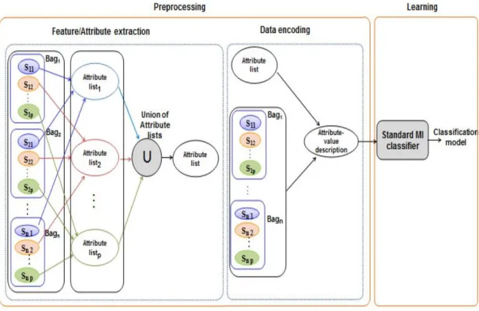
The simplest way to solve the problem of MIL for sequence data is to use standard MIL classifiers. The naive approach contains two steps (see Figure 1). We first make a preprocessing step that transforms the set of sequences to an attribute-value matrix where each row corresponds to a bag of sequences and attributes conform the columns. The second step consists in applying an existing MIL classifier. In the case of sequence data, the most used technique to transform data to an attribute-value format is to extract motifs that serve as attributes/features. We note that finding a uniform description of all instances using a set of motifs is not always an easy task. Since our naive approach takes into account the across bag relations between instances, the preprocessing step extracts motifs from each set of related instances. The union of these extracted motifs is then used as features to construct an attribute-value matrix where each row corresponds to a bag. The presence or the absence of an attribute in a sequence is respectively denoted by 1 or 0. Using this approach, we obtain an attribute-value matrix that contains a large number of motifs. It is worthwhile to mention that only a subset of the used attributes is representative for each processed sequence. Therefore, we may have a big sparse matrix when trying to present the whole sequence data using an attribute value format.
We apply the naive approach to our running example. We suppose that attributes are subsequences (minimum length = 2) that occur at least in 2 instances. Let AttributeList1 = {AB, CD, YZ} be the list of features extracted from the instances {Bi1, i=1, …, 4}. AttributeList2 = {EF, GH} is the list of features extracted from the instances {Bi2; i = 1, …, 5} and AttributeList3 = {KL} is the list of features extracted from the instances {Bi3, i ∈ {1, 4, 5}}. The union of the extracted motifs produces the list AttributeList = {AB, CD, YZ, EF, GH, KL}. In order to encode the learning sequence data, we generate the following attribute-value matrix denoted M:
1st instance 2nd instance 3rd instance M= ( 1 1 0 0 0 0 | 0 0 0 1 1 0 | 0 0 0 0 0 0 1 1 0 0 0 0 | 0 0 0 1 1 0 | - - - - - -0 1 1 -0 -0 -0 | -0 -0 -0 -0 1 -0 | - - - - - -1 0 -1 0 0 0 | -1 0 0 -1 0 0 | 0 0 0 0 0 -1 - - - - - - | 0 0 0 1 1 0 | 1 0 0 0 0 1 ) B1 B2 B3 B4 B5
The sparsity percentage of M is 77.2%. If we have a big learning database, M could result to a huge and sparse matrix since only a subset of the used subsequences is representative for each processed sequence.
Figure 1 System overview of the naive approach for MIL in sequence data
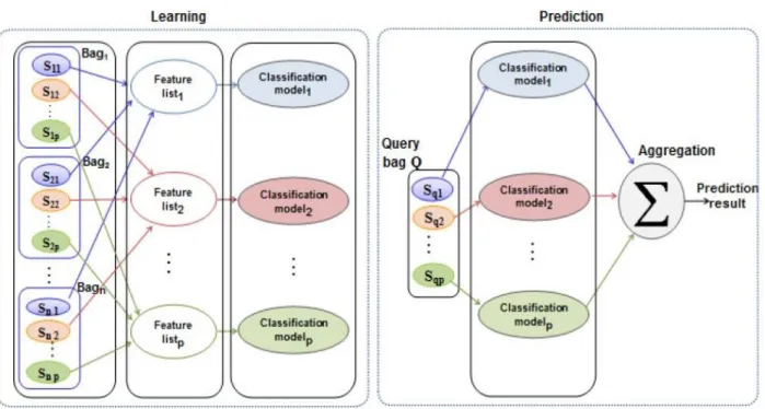
4.2. ABClass: Across Bag sequences Classification approach
ABClass takes advantage of the across bag relationship between sequences in order to reduce the number of attributes that are not representative for each processed sequence during the encoding step. Figure 2 represents the system overview of ABClass. Each set of related instances is presented by its own motifs vector. This relationship is also used during the learning step when generating partial models. Every vector of motifs will be used to produce a partial prediction result. These results will be then aggregated to compute the final result. Based on the formalization, the algorithm discriminates bags by applying a classification model to each instance of the query bag.
Algorithm 1 ABClass
Input: Learning database DB = {(Bi, Yi) , i= 1, …, n}, Query bag Q = {Qk, k= 1,
…, q}
Output: Prediction result P 1: for all Qk∈ Q do
2: AcrossBagSeqListk AcrossBagSeq (k, DB) 3: MotifListk MotifExtractor (AcrossBagsListk) 4: Mk EncodeData (MotifListk, AcrossBagsListk) 5: Modelk GenerateModel (Mk) 6: QVk EncodeData (MotifListk, Qk) 7: PVk ApplyModel (QVk, Modelk) 8: end for 9: P Aggregate (PV) 10: return P
Figure 2 System overview of the ABClass approach
ABClass is described in Algorithm 1. The acrossBagSeq function groups the related instances among bags into a list. During the execution of the algorithm, we will use the following variables:
- A matrix M to store the encoded data of the learning database. - A vector QV to store the encoded data of the query bag. - A vector PV to store the partial prediction results. Informally, the main steps of the ABClass algorithm are:
1. For each instance sequence Qk in the query bag Q, the related instances among bags of the learning database are grouped into a list (lines 1 and 2).
2. The algorithm extracts motifs from the list of grouped instances. These motifs are used to encode instances in order to create a discriminative model (lines 3 to 5).
3. ABClass uses the extracted motifs to represent the instance Qk of the unknown bag into a vector
QVk, then it compares it with the corresponding model. The comparison result is stored in the kth element of a vector PV (lines 6 and 7).
4. An aggregation method is applied to PV in order to compute the final prediction result P (line 9), which consists in a positive or a negative class label.
We apply the ABClass approach to our running example. Since the query bag contains 3 instances Q1, Q2 and Q3, we need 3 iterations followed by an aggregation step.
Iteration 1: ABClass groups the set of bags that are related and extract the corresponding motifs.
AcrossBagsList1 = {B11, B21, B31, B41}
MotifList1 = {AB, CD, YZ}
Then, it generates the attribute-value matrix M1 describing the sequences related to Q1.
AB CD YZ M1= ( 1 1 0 1 1 0 0 1 1 1 0 1 ) B11 B21 B31 B41
The sparsity percentage of the produced matrix M1 is reduced to 33% because there is no need to use the motifs extracted from instances {B i2, i = 1, .., 5} and {Bi3, i ∈ {1, 4 , 5}} to describe the instances {B i1,
i = 1, .., 4}. A model is then created using the encoded data and a vector QV1 is generated to describe Q1. QV1= (
1 1 0
)
By applying the model to the vector QV1, we obtain the first partial prediction result and we store it into the vector PV.
PV1 ← ApplyModel (QV1, Model1)
Iteration 2: The second iteration concerns the second instance Q2 of the query bag. We do the same instructions described in the first iteration.
AcrossBagsList2 = {B12, B22, B32, B42, B52}
Motif List2 = {EF, GH}
EF GH M2= ( 1 1 1 1 0 1 1 0 1 1) B12 B22 B32 B42 B52 QV2= (11) PV2 ← ApplyModel (QV2, Model2) Iteration 3: Only B1, B4 and B5 have related instances to Q3.
AcrossBagsList3 = {B13, B43, B53} Motif List3 = {KL} KL M3= ( 0 1 1 ) B13 B43 B53 QV3=(1) PV3 ← ApplyModel (QV3, Model3)
The aggregation step is finally used to generate the final prediction decision using the partial prediction results. We opt for the majority vote.
4.3. ABSim: Across Bag sequences Similarity approach
According to the specificity of the processed data, a similarity measure can be defined and used to discriminate instances. We propose an algorithm that focuses on discriminating bags by measuring the similarity between each sequence in the query bag and its corresponding related sequences in the different bags of the learning database. ABSim was originally presented in (Aridhi et al. 2016) as an algorithm used for IRR prediction. When applied on genomic sequences, ABSim uses the alignment score as similarity measure to compare protein sequences.
Algorithm 2 ABSim
Input: Learning database DB = {(Bi, Yi), i= 1, …, n}, Query bag Q = {Qk, k = 1,
…, q}
Output: Prediction result P 1: for all Qk∈ Q do 2: for all Bi∈ DB do
3: Mik similarityMeasure (Qk, Bik) /*Bik is the instance number k in the bag Bi*/
4: end for 5: end for
6: P Aggregate (M )
7: return P
ABSim works as described in Algorithm 2. Let M be a matrix used to store similarity measurement score vectors during the execution of the algorithm. Informally, the algorithm is described as follows:
1. For each instance sequence Qk in the query bag Q, it computes the corresponding similarity scores (line 1 to 5). The similarity scores of all instances of the query bag are grouped into a matrix M (line 3). The element Mik corresponds to the similarity score between Qk of Q and Bik of
Bi.
2. An aggregation method is applied to M in order to compute the final prediction result P (line 6). According to the aggregation result, a class label is associated to the query Bag.
Two aggregation methods are defined: Sum of Maximum Scores (SMS) and Weighted Average of Maximum Scores (WAMS). Algorithms 3 and 4 illustrate the SMS and WAMS aggregation methods. For each sequence in the query bacterium, we scan the corresponding line of M, which contains the obtained scores against all the other bags of the training database. The SMS method selects the maximum score among the similarity scores against bags that belong to the positive class label (which we call maxP ) and the maximum score among the similarity scores against bags that belong to the negative class label (which we call maxN). These scores are then compared. If maxP is greater than maxN, it adds maxP to the total score of the positive class label (which we denote totalP (M)). Otherwise, it adds maxN to the total score of the negative class label (which we denote totalN (M)). When all selected sequences were processed, the SMS method compares total scores of positive class label and negative class label. If
totalP (M) is greater than totalN (M), the prediction output is the positive class label. Otherwise, the prediction output is the negative class label.
Using the WAMS method, each sequence Qi has a given weight wi. For each sequence in the query bag, we scan the corresponding line of M, which contains the obtained scores against all other bags of the training database. The WAMS method selects the maximum score among the similarity scores against bags that belong to positive class label (which we denote maxP (M)) and the maximum score among the similarity scores against bags that belong to the negative class label (which we denote maxN (M)). It then compares these scores. If the maxP (M) is greater than maxN (M), it adds maxP (M) multiplied by the weight of the sequence to the total score of the positive class label and it increments the number of positive bags having a max score. Otherwise, it adds maxN (M) multiplied by the weight of the sequence to the total score of the negative class label and it increments the number of negative bags having a max score. When all the selected sequences were processed, we compare the average of total scores of positive class labels (which we denote avg (M)) and the average of total scores of negative class labels
(which we denote avgN (M)). If avgP (M) is greater than avgN (M), the prediction output is the positive class label. Otherwise, the prediction output is the negative class label.
Algorithm 3 SMS Algorithm 4 WAMS
Input: Similarity matrix M= {Mij, i= 1, …, n and j= 1,
…, p}
Output: A prediction result P 1: totalP 0 2: totalN 0 3: for i ∈ [1, n] do 4: maxP 0 5: maxN 0 6: for j ∈ [1, p] do
7: if Yj = +1 and maxP ≥ Mij then
8: maxP Mij
9: else if Yj = -1 and maxN ≥ Mij then 10: maxN Mij
11: end if 12: end for
13: if maxP ≥ maxN then
14: totalP totalP + maxP 15: else
16: totalN totalN + maxN 17: end if
18: end for
19: if totalP ≥ totalN then 20: P +1
21: else 22: P -1
23: end if 24: return P
Input: Similarity matrix M= {Mij, i= 1, … , n and j=
1, …, p}, Weight vector W = {(Wi, i= 1, …, p} Output: A prediction result P
1: totalP 0, totalN 0, nbP 0, nbN 0 2: for i ∈ [1, p] do
3: maxP 0 4: maxN 0 5: for j ∈ [1, n] do
6: if Yj = +1 and maxP ≥ Mij then
7: maxP Mij
8: else if Yj=-1and maxN≥ Mij then
9: maxN Mij
10: end if
11: end for
12: if maxP ≥ maxN then
13: totalP totalP + (maxP . wi) 14: nbP nbP + 1
15: else
16: totalN totalN + (maxN . wi) 17: nbN nbN + 1
18: end if 19: end for
20: avgP (M) totalP / nbP 21: avgN(M) totalN / nbN 22: if avgP (M) ≥ avgN (M) then 23: P +1
24: else 25: P -1
26: end if 27: return P
In order to apply the ABSim approach to our running example, we use a simple similarity measure that consists on computing the number of common symbols between the sequences. The first iteration computes the common symbols between the instance Q1 of the query bag and the four related instances
B11, B21, B31 and B41 and stores the results in the first column of the matrix M.
M = ( 4 - -4 - - 5 - - 3 - - - - - ) B1 B2 B3 B4 B5
M = ( 4 5 0 4 4 - 5 3 - 3 3 3 - 6 2 ) B1 B2 B3 B4 B5
Using the SMS aggregation method, we have the following results:
totalP (M ) = 0
totalN (M ) = 14
The query bag Q is finally classified as negative. In order to use the WAMS aggregation method, we need to specify a weight value for each instance. We suppose that all sequences are equally weighted, then we have the following results:
avgP (M ) = 0
avgN (M ) = 4.66
The query bag Q is finally classified as negative.
5. Experiments
We applied the naive approach, ABClass and ABSim to solve the problem of IRR prediction in bacteria. Ionizing-radiation-resistant bacteria (IRRB) are important in biotechnology. They could be used for bioremediation of radioactive wastes and in the therapeutic industry. The proposed MIL-based prediction systems aim to affiliate an unknown bacterium to either IRRB or ionizing-radiation-sensitive bacteria (IRSB).
5.1. Experimental environment
For our tests, we used the dataset described in (Aridhi et al. 2016). This dataset consists of 28 bags. Each bag/bacterium contains 25 to 31 instances that correspond to proteins implicated in basal DNA repair in IRRB. Bacteria represent the bags and primary structures of basal DNA repair proteins represent the instances. The used across bag relation is the orthology. Orthologous genes are assumed to have the same biological functions in different species. In the preprocessing step, we used the perfectBLAST (Santiago-Sotelo and Ramirez-Prado 2012) tool to identify orthologous proteins. We note that some proteins do not have any ortholog in some bags. We do not have the same number of instances in each bag.
Additional and more detailed information about our datasets and our experiments can be found in the following link: http://homepages.loria.fr/SAridhi/software/MIL/ . We used WEKA (Hall et al. 2009) data mining tool in order to apply existing well-known classifiers to test the proposed approaches. The similarity measure used when applying the ABSim approach is the local alignment score. We used BLAST (Altschul et al. 1990) to compute this score.
5.2. Experimental protocol
Experiments were carried out using the LOO technique. In order to evaluate ABClass and the naive approach, we need to encode the protein sequences of each bag using a set of features/motifs. We generated these motifs using the DMS motif extraction method (Maddouri and Elloumi, 2004). DMS allows building motifs that can discriminate a family of proteins from other ones. It first identifies motifs in the protein sequences. Then, the extracted motifs are filtered in order to keep only the discriminative and minimal ones. A substring is considered to be discriminative between the family F and the other families if it appears in F significantly more than in the other families. DMS extracts discriminative motifs according to α and β thresholds where α is the minimum rate of motif occurrences in the sequences of a family F and β is the maximum rate of motif occurrences in all sequences except those of the family F. In the following, we present the used motif extraction settings according to the values of α and β:
- S3 (α = 0.5 and β = 1): used to extract motifs having medium frequencies without discrimination.
- S4 (α = 0 and β = 1): used to extract infrequent and non discriminative motifs. - S5 (α = 1 and β = 0): used to extract frequent and strictly discriminative motifs.
5.3. Experimental results
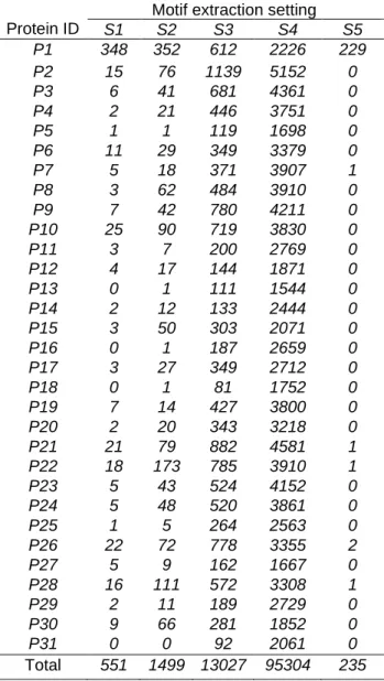
Table 1 presents, for each value of α and β, the number of extracted motifs from each set of related sequences (i.e., orthologous proteins). For the setting S5, there are no frequent and strictly discriminative motifs found for most proteins. That is why we will not use these values of α and β for our next experiments. We note that the number of extracted motifs increases for high values of β and low values of
α. As presented in Table 1, the number of infrequent and non discriminative motifs is very high. When
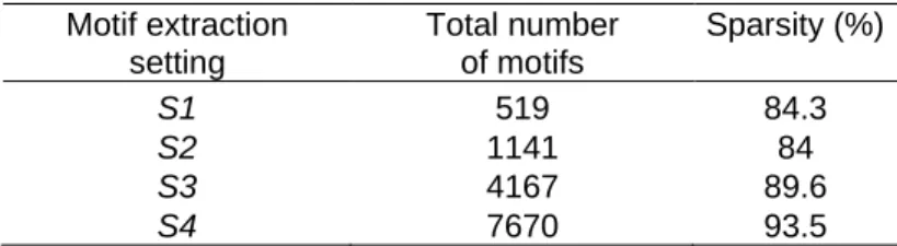
applying the naive approach, we first encode the data using the union of the extracted motifs from each set of related sequences. We show in Table 2 the sparsity of the attribute-value matrix which measures the fraction of zero elements over the total number of elements. The sparsity is generally proportional to the number of used motifs. For example, it goes from 84% with 1141 motifs to 93.5% with 7670 motifs.
Table 1 Number of extracted motifs for each set of orthologous proteins using a minimum motif length = 3
Protein ID
Motif extraction setting
S1 S2 S3 S4 S5 P1 348 352 612 2226 229 P2 15 76 1139 5152 0 P3 6 41 681 4361 0 P4 2 21 446 3751 0 P5 1 1 119 1698 0 P6 11 29 349 3379 0 P7 5 18 371 3907 1 P8 3 62 484 3910 0 P9 7 42 780 4211 0 P10 25 90 719 3830 0 P11 3 7 200 2769 0 P12 4 17 144 1871 0 P13 0 1 111 1544 0 P14 2 12 133 2444 0 P15 3 50 303 2071 0 P16 0 1 187 2659 0 P17 3 27 349 2712 0 P18 0 1 81 1752 0 P19 7 14 427 3800 0 P20 2 20 343 3218 0 P21 21 79 882 4581 1 P22 18 173 785 3910 1 P23 5 43 524 4152 0 P24 5 48 520 3861 0 P25 1 5 264 2563 0 P26 22 72 778 3355 2 P27 5 9 162 1667 0 P28 16 111 572 3308 1 P29 2 11 189 2729 0 P30 9 66 281 1852 0 P31 0 0 92 2061 0 Total 551 1499 13027 95304 235
Table 2 Sparsity of the attribute-value matrix generated for the naive approach Motif extraction setting Total number of motifs Sparsity (%) S1 519 84.3 S2 1141 84 S3 4167 89.6 S4 7670 93.5
Both ABClass and ABSim approaches provide good overall accuracy results compared to those obtained using the naive approach (see Figure 3). This shows that our proposed approaches are efficient. The results provided by ABSim using the SMS aggregation method are slightly better than those obtained using WAMS. The best result is reached using ABClass approach and the motif extraction settings S1, S2 and S3. Using these three settings, a minimum threshold of frequency and/or discrimination should be reached when extrcating motifs. The figures Figure 3 (a) and Figure 3 (b) show the impact of the motif extraction settings on the prediction results using the naive approach and ABClass. For example, using MISVM classifier, the accuracy varies from 53.5% using S1 to 82.1% using S3. Although the motifs extracted using S1 are discriminative, the naive approach does not provide good accuracy results for most multiple instance classifiers. For some classifiers, the results using S1 are the lowest comparing with the other motif extraction settings. However, using this setting, ABClass provides good results since it reaches 100% of accuracy using SVM, SMO and IBk classifiers, 96.4% using Logistic and 93.3% using J48. This could be explained by the fact that the naive approach looses the advantage of representing the instances using discriminative motifs when it uses the union of all motifs in the data encoding step. Using S4, ABClass does not reach 100% of accuracy although it succeeds to reach it with some classifiers using the other three settings S1, S2 and S3. No constraints related to frequency (α = 0) or discrimination (β = 1) were required when extracting motifs using S4.
(a) Naive approach
(b) ABClass (c) ABSim
Figure 3 Accuracy results 0 10 20 30 40 50 60 70 80 90 100 S1 S2 S3 S4 MISVM MISMO MILR CitationkNN MITI QuickDDIterative 0 10 20 30 40 50 60 70 80 90 100 S1 S2 S3 S4 SVM SMO Logistic IBk J48 0 10 20 30 40 50 60 70 80 90 100 SMS WAMS
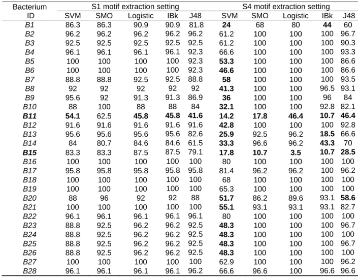
We compute the rate of classification models that contribute to predict the true class of each bacterium using ABClass approach (see Table 3). We present this rate for the motif extraction setting that provides the best accuracy rates i.e., S1 and the setting that provides low accuracy pourcentages, i.e., S4. The rate of successful classification models that does not exceed 60% are marked with bold text. The two bacteria B11 and B15 often generate low rates. We note that the results are similar to those found in (Aridhi et al. 2016). Although B11 is sometimes successfully classified, its higher successful classification rate does not exceed 62.5%. The rate of B15 does not reach 30% using S4. These results may help to understand some characteristics of the studied bacteria, in particular M. radiotolerans (B11) and B. abortus (B15) that present the lowest rates. A possible biological explanation is provided in (Zoghlami et
al. 2018; Aridhi et al. 2016) and notes that this could be explained by the increased rate of sequence
evolution in endosymbiotic bacteria (Woolfit and Bromham 2003).
Table 3 Rate of successful classification models using ABClass approach and LOO evaluation method
Bacterium ID
S1 motif extraction setting S4 motif extraction setting
SVM SMO Logistic IBk J48 SVM SMO Logistic IBk J48
B1 86.3 86.3 90.9 90.9 81.8 24 68 80 44 60 B2 96.2 96.2 96.2 96.2 96.2 61.2 100 100 100 96.7 B3 92.5 92.5 92.5 92.5 92.5 61.2 100 100 100 90.3 B4 96.1 96.1 96.1 96.1 92.3 66.6 100 100 100 93.3 B5 100 100 100 100 92.3 53.3 100 100 100 86.6 B6 100 100 100 100 92.3 46.6 100 100 100 86.6 B7 88.8 88.8 92.5 92.5 88.8 58 100 100 100 93.5 B8 92 92 92 92 92 41.3 100 100 96.5 93.1 B9 95.6 92 91.3 91.3 86.9 36 100 100 96 84 B10 88 100 88 88 84 32.1 100 100 92.8 82.1 B11 54.1 62.5 45.8 45.8 41.6 14.2 17.8 46.4 10.7 46.4 B12 91.6 91.6 91.6 91.6 91.6 42.8 100 100 100 92.8 B13 95.6 95.6 95.6 95.6 82.6 25.9 92.5 96.2 18.5 66.6 B14 84 80.7 84.6 84.6 61.5 33.3 96.6 96.2 43.3 70 B15 83.3 83.3 87.5 87.5 79.1 17.8 10.7 3.5 10.7 28.5 B16 100 100 100 100 100 80 100 100 100 100 B17 95.8 95.8 95.8 95.8 95.8 81.4 96.2 96.2 100 96.2 B18 100 100 100 100 100 68 100 100 100 100 B19 100 100 100 100 100 65.3 100 100 100 100 B20 88 96 92 92 88 51.7 86.2 89.6 93.1 58.6 B21 100 100 100 100 100 55.1 93.1 93.1 93.1 82.7 B22 96.1 96.1 96.1 96.1 96.1 80 100 100 100 100 B23 88.8 92.5 96.2 96.2 92.5 48.3 100 100 100 96.7 B24 88.8 92.5 96.2 96.2 92.5 48.3 100 100 100 100 B25 88.8 92.5 96.2 96.2 92.5 48.3 100 100 100 96.7 B26 88.8 92.5 96.2 96.2 92.5 48.3 100 100 100 100 B27 100 100 100 100 100 62.9 100 100 100 96.2 B28 96.1 96.1 96.1 96.1 96.2 66.6 96.6 100 96.6 96.6
6. Conclusion
In this paper, we addressed the issue of MIL in the case of sequence data. We focused on data that present relationships between instances of different bags. We described two novel approaches for MIL in sequence data with across bag dependencies. In the first method, called ABClass, each set of related instances will be presented by its own motifs vector. A discriminative classifier is then applied to compute a partial classification result. The second method, called ABSim, uses a matrix to store similarity
measurement score vectors to discriminate the related instances. Both methods apply an aggregation step in order to generate the final classification result. We applied ABClass and ABSim to solve the problem of IRR prediction in bacteria. By running experiments, we have shown that the proposed approaches are efficient. A better accuracy result could be provided by ABClass according to the used settings. In the future work, we will study how the use of a priori knowledge can improve the efficiency of the presented approaches. We specifically want to define weights for sequences by using a priori knowledge in the learning phase. Another avenue is to tackle this problem through protein 3D structure based on the work reported in (Dhifli et al. 2014).
References
Alpaydin E, Cheplygina V, Loog M, Tax D M (2015) Single-vs. multiple-instance classification. Pattern Recognition, 48(9):2831–2838.
Altschul S F, Gish W, Miller W, Myers E W, Lipman D J (1990) Basic local alignment search tool. Journal of molecular biology, 215(3):403–410.
Amores J (2013) Multiple instance classification: Review, taxonomy and comparative study. Artificial Intelligence, 201:81–105.
Amores J (2015). MILDE: multiple instance learning by discriminative embedding. Knowledge and Information Systems, 42(2):381–407.
Andrews S, Tsochantaridis I, Hofmann T (2003) Support Vector Machines for Multiple-Instance Learning. In: Advances in Neural Information Processing Systems, pp 561–568.
Aridhi S, Sghaier H, Zoghlami M, Maddouri M, Mephu Nguifo E (2016) Prediction of ionizing radiation resistance in bacteria using a multiple instance learning model. Journal of Computational Biology, 23(1):10–20.
Blekas K, Fotiadis D I, Likas A (2005) Motif-based protein sequence classification using neural networks. Journal of Computational Biology, 12(1):64–82.
Cheng B Y M, Carbonell J G, Klein-Seetharaman J (2005) Protein classification based on text document classification techniques. Protein : Structure, Function, and Bioinformatics, 58(4) :955–970.
Dhifli W, Saidi R, Mephu Nguifo E (2014) Smoothing 3D protein structure motifs through graph mining and amino acid similarities. Journal of Computational Biology, 21(2):162–172.
Fang G, Bhardwaj N, Robilotto R, Gerstein M B (2010) Getting started in gene orthology and functional analysis. PLoS computational biology, 6(3):e1000703.
Faria A W, Coelho F G, Silva A, Rocha H, Almeida G, Lemos A P, Braga A P (2017) MILKDE : A new approach for multiple instance learning based on positive instance selection and kernel density estimation. Engineering applications of artificial intelligence, 59:196–204.
Foulds J, Frank E (2010) A review of multi-instance learning assumptions, The knowledge engineering review, 25:1–25.
Hall M, Frank E, Holmes G, Pfahringer B, Reutemann P, Witten I H (2009) The Weka data mining software : an update. ACM SIGKDD explorations newsletter, 11 (1):10–18.
Herrera F, Ventura S, Bello R, Cornelis C, Zafra A, Sanchez-Tarrago D, Vluymans S (2016). Multiple Instance Learning: Foundations and Algorithms. Springer.
Kim J, Moriyama E N, Warr C G, Clyne P J, Carlson J R (2000) Identification of novel multi-transmembrane proteins from genomic databases using quasi-periodic structural properties. Bioinformatics, 16(9) :767–775.
Lesh N, Zaki M J, Ogihara M (1999) Mining features for sequence classification. In: Proceedings of the fifth international conference on knowledge discovery and data mining, pp 342–346.
Li Z, Geng GH, Feng J, Peng JY, Wen C, Liang JL (2014) Multiple instance learning based on positive instance selection and bag structure construction. Pattern recognition letters, 40:19–26.
Maddouri M, Elloumi M (2004) Encoding of primary structures of biological macromolecules within a data mining perspective. Journal of Computer Science and Technology, 19(1):78–88.
Maron O, Lozano-Pérez T (1998) A Framework for Multiple-Instance Learning. Advances in Neural Information Processing Systems, 10:570–576.
Melki G, Cano A, Ventura S (2018) MIRSVM: Multi-instance support vector machine with bag representatives. Pattern Recognition, 79: 228-241.
Needleman S B, Wunsch C D (1970) A general method applicable to the search for similarities in the amino acid sequence of two proteins. Journal of molecular biology, 48(3):443–453.
Saidi R, Aridhi S, Mephu Nguifo E, Maddouri M (2012) Feature extraction in protein sequences classification: a new stability measure. In: Proceedings of the ACM Conference on Bioinformatics, Computational Biology and Biomedicine, pp 683-689.
Saidi R, Maddouri M, Mephu Nguifo E (2010) Protein sequences classification by means of feature extraction with substitution matrices. BMC Bioinformatics. https://doi.org/10.1186/1471-2105-11-175 Saigo H, Vert JP, Ueda N, Akutsu T (2004) Protein homology detection using string alignment kernels. Bioinformatics, 20(11):1682–1689.
Santiago-Sotelo P, Ramirez-Prado J H (2012) prfectBLAST : a platform-independent portable front end for the command terminal BLAST+ stand-alone suite. BioTechniques, 53(5):299–300.
Sarker B, Ritchie D W, Aridhi S (2018) Exploiting complex protein domain networks for protein function annotation. In: Aiello L, Cherifi C, Cherifi H, Lambiotte R, Lió P, Rocha L (eds) Complex networks and their applications VII, pp 598-610.
Srivastava P K, Desai D K, Nandi S, Lynn A M (2007) Hmm-mode–improved classification using profile hidden markov models by optimising the discrimination threshold and modifying emission probabilities with negative training sequences. BMC bioinformatics, 8(1): 104 -121.
Sutskever I, Vinyals O, Le Q V (2014) Sequence to sequence learning with neural networks. In: Advances in neural information processing systems, pp 3104–3112.
Tao Q, Scott S, Vinodchandran N, Osugi T T (2004) SVM-based generalized multiple-instance learning via approximate box counting. In: Proceedings of the twenty first international conference on machine learning, pp 779–806
Wang J (2000) Solving the multiple-instance problem: A lazy learning approach. In: Proceedings of the seventeenth international conference on machine learning, pp 1119–1125.
Woolfit M, Bromham L (2003) Increased rates of sequence evolution in endosymbiotic bacteria and fungi with small effective population sizes. Molecular Biology and Evolution, 20(9):1545–1555.
Wei X-S, Wu J, Zhou Z-H (2017). Scalable algorithms for multi-instance learning. IEEE Transactions on Neural Networks and Learning Systems, 28(4):975–987.
Xing Z, Pei J, Keogh E (2010) A brief survey on sequence classification. ACM SIGKDD Explorations Newsletter, 12(1):40–48.
Yakhnenko O, Silvescu A, Honavar V (2005) Discriminatively trained markov model for sequence classification. In: Proceedings of the fifth IEEE International Conference on Data Mining, pp 8-16.
Yuan J, Huang X, Liu H, Li B, Xiong W (2016). Submil: Discriminative subspaces for multi-instance learning. Neurocomputing, 173:1768–1774.
Zhang D, Liu Y, Si L, Zhang J, Lawrence R D (2011) Multiple instance learning on structured data. In: Advances in Neural Information Processing Systems, pp 145–153.
Zhou Z-H, Sun Y-Y, and Li Y-F (2009). Multi-instance learning by treating instances as non-iid samples. In: Proceedings of the twenty sixth International Conference on Machine Learning, pp 1249–1256. Zoghlami M, Aridhi S, Maddouri M, Mephu Nguifo E (2018) An overview of in silico methods for the prediction of ionizing radiation resistance in bacteria. In: Ionizing Radiation: Advances in Research and Applications, Physics Research and Technology Series, pp 241-256.