en fr

HAL Id: hal-03205628

https://hal-univ-tlse3.archives-ouvertes.fr/hal-03205628

Submitted on 22 Apr 2021

HAL is a multi-disciplinary open access

archive for the deposit and dissemination of

sci-entific research documents, whether they are

pub-lished or not. The documents may come from

teaching and research institutions in France or

abroad, or from public or private research centers.

L’archive ouverte pluridisciplinaire HAL, est

destinée au dépôt et à la diffusion de documents

scientifiques de niveau recherche, publiés ou non,

émanant des établissements d’enseignement et de

recherche français ou étrangers, des laboratoires

publics ou privés.

Distributed under a Creative Commons Attribution| 4.0 International License

Human-Interpretable Rules for Anomaly Detection in

Time-series

Inès Ben Kraiem, Faiza Ghozzi, André Péninou, Geoffrey Roman-Jimenez,

Olivier Teste

To cite this version:

Inès Ben Kraiem, Faiza Ghozzi, André Péninou, Geoffrey Roman-Jimenez, Olivier Teste.

Human-Interpretable Rules for Anomaly Detection in Time-series. 24th International Conference on

Extend-ing Database Technology (EDBT 2021), University of Cyprus, Mar 2021, Nicosia (virtual), Cyprus.

pp.457-462, �10.5441/002/edbt.2021.51�. �hal-03205628�

Human-Interpretable Rules for Anomaly Detection in

Time-series

Ines Ben Kraiem

University of Toulouse - UT2J, IRIT Toulouse, France

ines.ben-kraiem@irit.fr

Faiza Ghozzi

University of Sfax- ISIMS, MIRACL Sfax, Tunisie

faiza.ghozzi@isims.usf.tn

Andre Peninou

University of Toulouse- UT2J, IRIT Toulouse, France andre.peninou@irit.fr

Geoffrey Roman-Jimenez

Olivier Teste

University of Toulouse- UT2J, IRIT Toulouse, France

olivier.teste@irit.fr

ABSTRACT

Human-interpretable rules for anomaly detection refer to ab-normal data presented in a format that cannot be intelligible to analysts. Learning these rules is a challenging issue, while only a few works address the problem of different types of anom-alies in time-series. This paper presents an extended decision tree based on patterns to generate a minimized set of human-comprehensible rules for anomaly detection in univariate time-series. This method uses Bayesian optimization to avoid manual tuning of hyper-parameters. We define a quality measure to eval-uate both the accuracy and the intelligibility of the produced rules. The performance of the proposed method is experimen-tally assessed on real-world and benchmark datasets. The results show that our approach generates rules that outperforms state-of-the-art anomaly detection techniques.

1

INTRODUCTION

Anomaly detection in time series is a widely studied issue in many areas such as financial markets, sensor networks, habitat monitoring, network intrusion, web traffic [1], and many others. Time series are often affected by unusual events or untimely changes (e.g., measurement error or faulty sensors) that need to be detected and processed by users for analysis and exploration [7].

In a real context, experts may observe some interesting local phenomena, which can be seen as remarkable points in time series. Using their domain knowledge, the experts investigate sequences of remarkable points to detect and locate anomalies. Experts can also build decision rules manually to detect future occurrences of these anomalies. However, as the amount of col-lected data is increasing, the decision rules become more complex to define which makes the analysis more difficult. Automatic rule extraction and detection of different types of anomalies can be of considerable interest to an expert, leading to appropriate action that can save a lot of time and value. To overcome this challenge, rule learning algorithms have been proposed [2, 12]. Deploying such systems might reveal comprehensible information to the users to explain the root cause of anomalies better than black-box algorithms.

To address these challenges, we provide a machine learning method to generate human-interpretable rules for anomaly de-tection in time-series, called Composition-based Decision Tree

© 2021 Copyright held by the owner/author(s). Published in Proceedings of the 24th International Conference on Extending Database Technology (EDBT), March 23-26, 2021, ISBN 978-3-89318-084-4 on OpenProceedings.org.

Distribution of this paper is permitted under the terms of the Creative Commons license CC-by-nc-nd 4.0.

(CDT)1. This method uses patterns to identify remarkable points.

The compositions of remarkable points existing into time-series are learned through a specific decision tree that finally produces intelligible rules. To avoid manual tuning, we use Bayesian hyper-parameter optimization to get the best hyper-hyper-parameters for our model. The approach aims at finding the best compromise be-tween a high accuracy during anomaly detection and a minimized set of easily human-interpretable rules. We conduct experiments on three real-world datasets and three synthetic datasets. The results show the effectiveness of our method compared to both pattern-based methods and rule-based methods for anomaly de-tection.

2

RELATED WORK

Numerous works on anomaly detection in time-series had been covered under various surveys and reviews [3, 13]. Several fields of study are related to pattern-based time-series data mining and rule-learning methods for anomaly detection. Pattern-based methods aim to discover frequent [4, 5] or infrequent sub-sequences [16] from a time-series. In contrast to our method, these methods are less suitable for detecting multiple anomalies and can only find a specific type of anomaly. Rule-learning methods aim to find regularities in data that can be expressed in the form of IF-THEN-like rules [2, 9, 11]. In general, the rules are evaluated based on accuracy or the number of rules produced by these al-gorithms. In this paper, instead of only evaluating the rules based on these criteria, we introduce a quality measure, which takes into account the number of used patterns as well as the length of rules, to make the rules simpler to interpret. We also propose a function that seeks a compromise between the interpretability of the rules and their precision.

3

METHODOLOGY

In this section, we describe our Composition-based Decision Tree (CDT) method for anomaly detection and rule extraction.

3.1

Time-Series Preprocessing

Definition 1. An univariate time-series is defined as𝑇 𝑠 = {𝑥1, ..., 𝑥𝑛}

where ∀𝑖 ∈ [1..𝑛], 𝑥𝑖∈ R such that values 𝑥𝑖are uniformly spaced

in time and 𝑛 is the size of 𝑇 𝑠.

The time series are collected from different sensors and the values of measures are on different ranges. To achieve scale and offset invariance, we normalize each continuous time-series 𝑇 𝑠 to values within the range [0, 1]. Resampling could also be used to provide additional structure or to smooth time series and remove

any noise; e.g., downsampling reduces the frequency of time-series observations.

3.2

Time-Series Labeling

To detect anomalies, experts first analyze the neighborhood of a point (unusual variations) such as the point which precedes it and follows it to decide if is a remarkable point. Based on this idea, we label each point of the time series by checking every three successive points using patterns.

Let us considers three successive points such as 𝑥𝑖−1, 𝑥𝑖, 𝑥𝑖+1

of a time-series. Considering all possible variations between these three points, we define nine possible variations, which can occur between successive points, as listed in Table 1 namely, PP (Pos-itive Peak), PN (Negative Peak), SCP (Start Constant Pos(Pos-itive), SCN (Start Constant Negative), ECP (End Constant Positive), ECN (End Constant Negative), CST (Constant), VP (Variation Positive) and VN (Variation Negative). Each of these variations can have different magnitudes into [-1,1]. To identify fine variations of values between three points, we refine each variation by defining intervals of variations into [-1,1].

Hyper-parameter (𝛿). We denote 𝛿 the hyper-parameter used to distinguish the different magnitudes considered for each of the nine variations (PP, PN, SCP, SCN, ECP ECN, CP, VN, and CST).

𝛿allows the introduction of fine amplitude shifts in the

varia-tions to capture the shape complexity in time-series, typically small or large amplitudes. 𝛿 represents the number of disjointed sub-intervals considered in [-1,1] and will be determined automat-ically using Bayesian optimization. For a given 𝛿, we construct 2𝛿 + 1 intervals : i) 𝛿 sub-intervals for positive variations in ]0, 1], ii) 𝛿 intervals for negative variations in [−1, 0[, and iii) 1 special case for the absence of variation (equal to 0).

For the sake of simplicity, in the rest of the paper, we only consider notation with 𝛿 = 2 (other values of 𝛿 will only result in a larger variety of intervals and patterns), and we denote the 5 resulting intervals as follows: Low (L) = ]0,0.5], High (H) = ]0.5,1], -Low (-L) = [-0.5,0[, -High (-H) = [-1,-0.5[, and the special case,

Zero (Z) = 0.

Definition 2. We define a pattern annotated 𝑃 = (𝑙, 𝛼, 𝛽) where

𝑙is a name (or label) identifying the pattern, and 𝛼 and 𝛽 are

two possible intervals from [-1,1]. For each successive points

𝑥𝑖−1, 𝑥𝑖, 𝑥𝑖+1, the point 𝑥𝑖is checked by a pattern only if 𝑥𝑖−𝑥𝑖−1∈

𝛼∧ 𝑥𝑖− 𝑥𝑖₊₁∈ 𝛽. In this case, 𝑥𝑖 is labeled with 𝑙. For the rest of

the paper, labels are denoted by the name of the variation (PP, PN, etc.).

Fig. 1 (left) illustrates an example of a pattern 𝑃𝑃𝐿,𝐻 that helps

us to find one remarkable point from a series. This time-series represents the consumption data of a building’s calorie sensor. Fig. 1 (right) shows examples of different magnitudes of

pattern such as 𝑃𝑃𝐿,𝐻, 𝑃𝑃𝐿,𝐿and 𝑃𝑃𝐻 ,𝐻. Using these patterns,

we can automatically label each point in time series.

Figure 1: Example of different magnitudes of a pattern.

Definition 3. A labeled times-series annotated𝑇 𝑠𝑏 = {𝑙1, ..., 𝑙𝑁}

with 𝑁 = 𝑛 − 2 where each 𝑥𝑖point of the initial time-series (𝑇 𝑠)

is replaced by the label of its corresponding pattern. Table 1: Types of variation for labelling.

3.3

Composition-based Decision Tree

Given the time series labeling, we built an extension of the deci-sion tree based on pattern compositions to produce rules able to detect anomalies.

Classically, a decision tree is induced from observations com-posed of feature values and a class label. It is built by splitting the training data into subsets by choosing the feature which best partitions the training data according to an evaluation criterion (e.g., Shannon’s entropy, Gini index). This criterion characterizes the homogeneity of the subsets obtained by division of the data set. This process is recursively repeated on each derived subset until all instances in a subset belong to the same class label [10]. The classical decision tree considers features without any or-der when splitting the datasets. Conversely, in our approach, we would like to keep the order of the time series. Thus, our deci-sion tree is built, by considering nodes as pattern compositions (ordered sequences of remarkable points) with the highest in-formation gain. These compositions are calculated from a set of observations (sub-sequences of labeled time-series). The input of the tree is constructed by creating fixed sized sliding windows.

Definition 4. A set of observations annotated 𝐷 = {𝑑1, 𝑑₂, ...,

𝑑𝑁−𝜔+1} = {{𝑙1, ..., 𝑙𝜔}, {𝑙2, ..., 𝑙𝜔+1},..., {𝑙𝑁−𝜔+1, ..., 𝑙𝑁}}

repre-sents the result of cutting 𝑇 𝑠𝑏 by a sliding window of size 𝜔, and using a fixed step size equal to one. Let M be the number of classes of observations. In our context, we consider two classes (M = 2): the abnormal class (observation with anomaly), or the

normal class (observation without anomaly). Each 𝑑𝑖observation

To determine a probability distribution of the observations over the classes, we introduce an impurity measure of a set of

observations 𝐷𝑗 ⊆ 𝐷. In our method, we opt to the Gini index.

The Gini impurity index, annotated 𝐺 (𝐷𝑗), provides a measure of

the quality of 𝐷𝑗according to the distribution of the observations

into the classes. The impurity metric is minimal (equal to 0) if a set contains only observations of one class, and it is maximal (equal to 0.5) if the set contains equally observations of all classes. Hyper-parameter (𝜔). We denote 𝜔 <= 𝑁 /2 the window size to define observations. This hyper-parameter will be deter-mined automatically using Bayesian optimization.

From an observation with anomaly we can define a composition used to split a node into two sub-nodes.

Definition 5. A composition annotated 𝑐 is a sub-sequence of

labels of an observation 𝑑𝑖. We denote 𝑐 ⊆𝑜𝑑𝑖.

Example. Considering 𝑑 = {𝑙1, 𝑙₂, 𝑙₃, 𝑙₄, 𝑙₅, 𝑙₆}, some

compo-sitions are 𝑐 = {𝑙2, 𝑙₃, 𝑙₄} ⊆𝑜 𝑑, 𝑐 = {𝑙3, 𝑙2, 𝑙4} ⊈𝑜 𝑑, and 𝑐 =

{𝑙1, 𝑙₂, 𝑙₃, 𝑙₄, 𝑙₅, 𝑙₆} ⊆𝑜𝑑.

We also introduce additional notations: 𝑐 ∈𝑜 𝐷 when ∀𝑑 ∈

𝐷 , 𝑐⊆𝑜𝑑, and 𝑐 ∉𝑜𝐷when ∀𝑑 ∈ 𝐷, 𝑐 ⊈𝑜𝑑.

A decision tree is built based on features that have the highest Information Gain [10]. In CDT, the compositions are compared according to the information gain, noted 𝐼𝐺, they provide.

The entire flow of the CDT approach we proposed is described by Algorithm 1. This algorithm builds a decision tree; we de-fine a tree node as a quadruplet: observations (the set of obser-vations considered in this node), a composition (used to split observations in two child nodes), childTrue (the node of obser-vations satisfying the composition), and childFalse (the node of observations that do not satisfy the composition). An example corresponding to the root node is given in line 1. We introduce a function 𝑙𝑖𝑠𝑡 _𝑜 𝑓 _𝑎𝑙𝑙_𝑝𝑜𝑠𝑠𝑖𝑏𝑙𝑒_𝑐𝑜𝑚𝑝𝑜𝑠𝑖𝑡𝑖𝑜𝑛𝑠 () to compute all

compositions deduced from a set 𝐷𝑗(line 6). For each

composi-tion, we calculate the information gain to split a node (line 7–15).

At line 16, if 𝐺 (𝐷𝑗) ≠ 0 means that the set of observations of the

node is impure (observations are of different classes). Moreover,

𝑚𝑎𝑥𝐺 𝑎𝑖𝑛 ≠0 means that a composition that splits the set of

observations has previously been found: in this case, we create

a node 𝑁𝑖𝑛𝑐that will determine the positive branch of the node

(𝑐 ∈𝑜𝐷𝑗), whereas 𝑁𝑒𝑥 𝑐will be the negative one (𝑐 ∉𝑜 𝐷𝑗) (line

16–25). We repeat these steps until there are no more nodes to process (line 3–26).

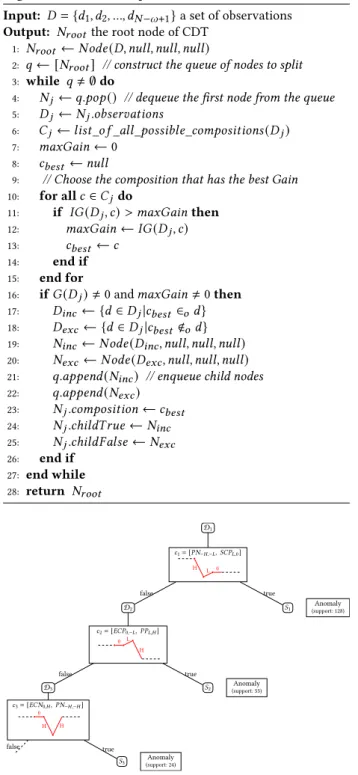
Example. Fig. 2 illustrates an example of CDT result. The

root-node is 𝐷1, and it represents the whole training set of

obser-vations used for the construction of the CDT. The leave-nodes represent class labels and branches represent conjunctions of compositions that lead to those class labels. As shown in Fig. 2, the CDT is composed of 3 splits constructing a set of 3 leaves

S = {𝑆1, 𝑆₂, 𝑆₃}.

3.4

Rule Generation for Anomaly Detection

We convert the CDT into a set of decision rules. We only consider “pure leaf-nodes” leading to the anomaly class.

Definition 6. A rule predicate, annotated 𝑅𝑠 is a branch of the decision tree leading to the anomaly class. It is constructed by

combining (conjunction) the successive compositions 𝑐𝑖or ¬𝑐𝑖

from the leaf-node to the root-node. For each positive branch

(𝑐𝑖 ∈𝑜 𝐷𝑗), the positive composition 𝑐𝑖 is deduced whereas a

negative composition ¬𝑐𝑖 is deduced from a negative branch

(𝑐𝑖 ∉𝑜𝐷𝑗).

Algorithm 1 CDT: Composition-based Decision Tree

Input: 𝐷 = {𝑑1, 𝑑₂, ..., 𝑑_{𝑁−𝜔+1}} a set of observations

Output: 𝑁𝑟 𝑜𝑜𝑡 the root node of CDT

1: 𝑁𝑟 𝑜𝑜𝑡 ← 𝑁 𝑜𝑑𝑒 (𝐷, 𝑛𝑢𝑙𝑙, 𝑛𝑢𝑙𝑙, 𝑛𝑢𝑙𝑙 )

2: 𝑞← [𝑁𝑟 𝑜𝑜𝑡] // construct the queue of nodes to split

3: while 𝑞 ≠ ∅ do

4: 𝑁𝑗 ← 𝑞.𝑝𝑜𝑝 () // dequeue the first node from the queue

5: 𝐷𝑗 ← 𝑁𝑗.𝑜𝑏𝑠𝑒𝑟 𝑣 𝑎𝑡 𝑖𝑜𝑛𝑠

6: 𝐶_𝑗← 𝑙𝑖𝑠𝑡 _𝑜 𝑓 _𝑎𝑙𝑙_𝑝𝑜𝑠𝑠𝑖𝑏𝑙𝑒_𝑐𝑜𝑚𝑝𝑜𝑠𝑖𝑡𝑖𝑜𝑛𝑠 (𝐷_𝑗)

7: 𝑚𝑎𝑥𝐺 𝑎𝑖𝑛← 0

8: 𝑐_{𝑏𝑒𝑠𝑡}← 𝑛𝑢𝑙𝑙

9: // Choose the composition that has the best Gain

10: for all 𝑐 ∈ 𝐶𝑗do 11: if 𝐼𝐺 (𝐷𝑗, 𝑐) > 𝑚𝑎𝑥𝐺𝑎𝑖𝑛then 12: 𝑚𝑎𝑥𝐺 𝑎𝑖𝑛← 𝐼𝐺 (𝐷𝑗, 𝑐) 13: 𝑐_{𝑏𝑒𝑠𝑡} ← 𝑐 14: end if 15: end for 16: if 𝐺 (𝐷𝑗) ≠ 0 and 𝑚𝑎𝑥𝐺𝑎𝑖𝑛 ≠ 0 then 17: 𝐷𝑖𝑛𝑐← {𝑑 ∈ 𝐷𝑗|𝑐𝑏𝑒𝑠𝑡∈𝑜𝑑} 18: 𝐷𝑒𝑥 𝑐 ← {𝑑 ∈ 𝐷𝑗|𝑐𝑏𝑒𝑠𝑡 ∉𝑜𝑑} 19: 𝑁𝑖𝑛𝑐← 𝑁 𝑜𝑑𝑒 (𝐷𝑖𝑛𝑐, 𝑛𝑢𝑙𝑙 , 𝑛𝑢𝑙𝑙 , 𝑛𝑢𝑙𝑙) 20: 𝑁𝑒𝑥 𝑐 ← 𝑁 𝑜𝑑𝑒 (𝐷𝑒𝑥 𝑐, 𝑛𝑢𝑙𝑙 , 𝑛𝑢𝑙𝑙 , 𝑛𝑢𝑙𝑙)

21: 𝑞 .𝑎𝑝 𝑝𝑒𝑛𝑑(𝑁𝑖𝑛𝑐) // enqueue child nodes

22: 𝑞 .𝑎𝑝 𝑝𝑒𝑛𝑑(𝑁𝑒𝑥 𝑐) 23: 𝑁𝑗.𝑐𝑜𝑚𝑝𝑜𝑠𝑖𝑡 𝑖𝑜𝑛← 𝑐𝑏𝑒𝑠𝑡 24: 𝑁_𝑗.𝑐ℎ𝑖𝑙𝑑𝑇 𝑟 𝑢𝑒← 𝑁_𝑖𝑛𝑐 25: 𝑁𝑗.𝑐ℎ𝑖𝑙𝑑 𝐹 𝑎𝑙 𝑠𝑒← 𝑁𝑒𝑥 𝑐 26: end if 27: end while 28: return 𝑁𝑟 𝑜𝑜𝑡 D1 𝑐1= [𝑃 𝑁−𝐻 ,−𝐿, 𝑆𝐶 𝑃𝐿,0] H _L 0 D2 𝑆1 𝑐₂= [𝐸𝐶𝑃0,−𝐿, 𝑃 𝑃𝐿,𝐻] 0 L H Anomaly (support: 128) 𝑆2 (support: 55)Anomaly D3 𝑐₃= [𝐸𝐶𝑁0,𝐻, 𝑃 𝑁−𝐻 ,−𝐻] 0 H H 𝑆3 (support: 24)Anomaly false false _true true false true

Figure 2: Illustration of a Composition-based Decision Tree (CDT).

Example. Three rules predicate are produced from the CDT in Fig. 2. • 𝑅𝑆₁: 𝑐1= [𝑃 𝑁−𝐻 ,−𝐿, 𝑆𝐶 𝑃𝐿,0] • 𝑅𝑆₂: 𝑐2∧ ¬𝑐1= [𝐸𝐶𝑃0,−𝐿, 𝑃 𝑃𝐿,𝐻] ∧ ¬[𝑃 𝑁−𝐻 ,−𝐿, 𝑆𝐶 𝑃_𝐿,0] • 𝑅𝑆₃: 𝑐3∧ ¬𝑐2∧ ¬𝑐1= [𝐸𝐶𝑁0,𝐻, 𝑃 𝑁−𝐻 ,−𝐻] ∧ ¬[𝐸𝐶𝑃0,−𝐿, 𝑃 𝑃𝐿,𝐻] ∧ ¬[𝑃 𝑁−𝐻 ,−𝐿, 𝑆𝐶 𝑃𝐿,0].

Using abusive notations, 𝑐𝑖∧¬𝑐𝑗means that for an observation

Definition 7. A rule, annotated R, is a disjunction of rule

predicates. For instance, as shown in Fig. 2, R = 𝑅𝑆₁∨ 𝑅𝑆₂∨ 𝑅𝑆₃=

(𝑐1) ∨ (𝑐2∧ ¬𝑐1) ∨ (𝑐3∧ ¬𝑐2∧ ¬𝑐1).

Rule Simplifications. One way to minimize CDT’s rules is to post-process the produced rules through Boolean algebra sim-plifications. We aim to minimize the “sum-of-products” forms of Boolean functions. In our approach, this inter-branch simplifica-tion is applied until there is no longer any simplificasimplifica-tion to be made. This allows us to minimize the number of compositions in a rule. Using Boolean algebra, we can simplify the rule R generated

from the tree in Fig. 2 as R = (𝑐1) ∨ (𝑐2∧¬𝑐1) ∨ (𝑐3∧¬𝑐2∧¬𝑐1) =

(𝑐1) ∨ (𝑐2) ∨ (𝑐3).

3.5

Quality Measure

We aim to generate rules that are both accurate and comprehensi-ble. According to experts opinion, a comprehensible rule should be short [2, 9] and should contain a minimized number of various labels. Therefore, we defined the following criteria to evaluate a quality of rules:

• I (𝑐) to characterize the quality of a composition 𝑐 depend-ing on its length and the number of patterns used;

• M (I𝑅𝑆) to characterize the quality of a rule predicate 𝑅𝑆

depending on the number of compositions and the quality of each one (I (𝑐));

• Q (R) to characterize the quality of a rule R depending on the quality of rule predicate and its support.

We first calculate the interpretability of a composition as:

I (𝑐) = 1 − 𝐿𝑐.𝑁𝐿

𝜔 .𝑀 𝑎𝑥 𝐿 (1)

where 𝐿𝑐 = |𝑐 | denotes the length of a composition 𝑐, 𝑁𝐿 is

the number of unique labels used in a composition, 𝜔 is the maximum window size, and 𝑀𝑎𝑥𝐿 is the total number of labels. Then, we calculate the average interpretability of a rule predicate (conjunction of compositions) as:

M (I𝑅𝑆) = 1 𝑁 𝑐 𝑁 𝑐 ∑︁ 𝑘=1 I (𝑐𝑘) (2)

where 𝑁 𝑐 is the number of compositions in a rule predicate 𝑅𝑆.

Finally, extracted rules’ quality is calculated as:

Q (R) = 1 𝑆 𝑛𝑏 ∑︁ 𝑖=1 𝑆𝑅𝑆𝑖 .M (I𝑅𝑆𝑖) (3)

where 𝑛𝑏 is the number of rule predicates in R, 𝑆𝑅𝑆𝑖is the support

of rule predicate (true positive) and 𝑆 is the support of all rules predicates (true positive and true negative). A rule predicate with high support is considered more important. Therefore, we multiplicate the average interpretability of a rule predicate with its support.

3.6

Hyper-Parameters selection

The manual tuning of hyper-parameters requires a prior knowl-edge. Automatic search algorithms such as grid search and ran-dom search could give good results. However, grid search is time consuming and random search might not find the optimal set. To address this problem, we use Bayesian Optimization [14] to efficiently get the best hyper-parameters (𝛿, 𝜔) for our model. Indeed, we aim to find a configuration (that is, a set of parame-ters) that maximizes a performance metric or an objective func-tion. Hence, we defined a search space and we try to find the hyper-parameters values of CDT that yield the highest result as

measured on a validation set. Hyper-parameter optimization is presented as:

ℎ∗=arg max

ℎ∈𝐻

𝐹(ℎ) (4)

where 𝐹 (ℎ) represents an objective function to maximize, ℎ∗ is the set of optimized hyper-parameters (𝛿, 𝜔) and ℎ can take any value in search space 𝐻 .

To optimize the trade-off between detection performance and good quality of rules, we defined the objective function 𝐹 (ℎ) as the F-measure weighted by our Q (R) rules’ quality measure.

𝐹(ℎ) = 𝐹 1(ℎ).Q (R) (5)

where 𝐹 1(ℎ) is the F-measure (the harmonic mean of the preci-sion and recall) of the classification performance obtained with the set of parameters (ℎ).

4

EXPERIMENTS

For our evaluation, we use real-world datasets from the Manage-ment and Exploitation Service (SGE) [6], and data from the Yahoo datasets [8]. We compare CDT with state-of-the-art pattern-based as well as rule-based methods for anomaly detection.

In SGE data sets, we aim to handle anomalies on calorie and electric consumption datasets. Calorie data consists of 25 con-sumption datasets from sensors deployed in different buildings managed by the SGE. These measurements are daily data for more than three years, about 33536 observations in total and they contain 586 anomalies. Electricity measurements are collected hourly for 10 years from one sensor (96074 in total). There are in total 10343 anomalies in the electricity dataset.

The Webscope S5 dataset, which is publicly available in [8], consists of 371 files divided into four categories, named A1/A2/A3/ A4, each one containing respectively, 67/100/100/100 files. A1 Benchmark is based on real production traffic from actual web services while classes A2, A3, and A4 contain synthetic anomaly data. These datasets are represented by time-series in one-hour units. There are a total of 94778 traffic values in 67 different files and 1669 of these values are abnormal. The anomalies in the syn-thetic datasets are inserted at random positions. A2 Benchmark contains 142002 values with 466 anomalies while 168000 values exist in A3 and A4 Benchmarks with respectively 943 and 837 anomalies.

4.1

Evaluation Process and Metrics

The performance of all the methods is compared based upon the F1 score, the rules’quality metric Q, and the objective func-tion 𝐹 (ℎ) used as defined in equafunc-tion (5). We use the 𝐹 1 score and Q score to compare the accuracy of our method against pattern-based methods. We use the 𝐹 (ℎ) score to evaluate both the accuracy and the interpretability of the rules generated by our CDT method compared to those of rule learning methods. For evaluation, we split every dataset into three subsets: training set (60%), validation set (20%), and testing set (20%) ratio. We use the train and validation set to optimize the model’s hyper-parameter values using Bayesian optimization. Then, we evaluate the optimized model on testing set.

Hyper-Parameters Optimization. To limit the search space of the Bayesian optimization, we constrained the parameter 𝜔 within [3,31] and 𝛿 within [1,21]. Table 2 shows the optimal hyper-parameters found with the Bayesian optimization. As we can see in Table 2, optimization on 𝐹 (ℎ) tends to favors a small number of splits (𝛿) for patterns when compared to the 𝐹 1 score optimization. This is due to the quality measure of rules Q (R),

which looks for short rules that include a minimum number of labels (𝛿). However, the size of observations (𝜔) needed to construct an optimal CDT remains to be comparable for 𝐹 1 and

𝐹(ℎ) suggesting the need for presence of neighbors surrounding

an anomaly to achieve good anomaly detection with CDT. Table 2: Parameters of CDT for experiments.

Evaluation F1-score F(h)-score

Dataset 𝜔 𝛿 𝜔 𝛿 SGE_Electricity 27 2 27 2 SGE_Calorie 5 4 21 1 Yahoo_A1 27 16 25 1 Yahoo_A2 17 2 17 1 Yahoo_A3 29 12 17 1 Yahoo_A4 25 8 21 1

4.2

Experiments with Pattern-based

Algorithms

We employ the following three approaches as baseline methods to compare with our approach:

• Pattern-Based Anomaly Detection (PBAD) is an anom-aly detection method based on frequent pattern mining techniques in mixed-type time-series [4].

• Matrix Profile (MP) is an anomaly detection method based on similarity-join to detect time series discords [15]. • Pattern Anomaly Value (PAV) is an anomaly detection

algorithm based on pattern anomaly value. The anomalies are the infrequent linear pattern [16] .

To evaluate these methods, we used the implementation avail-able in [4]. These algorithms are window-based approaches. Hence, we used the recommended settings for each of them. We split the time series into sliding windows of length 12 with a step size 6. These anomaly detection algorithms provide an anomaly score for each window. As these algorithms are unsupervised, we build the anomaly detection model on the full-time series data and we evaluate it using 𝐹 1 score. For CDT, we used the appropriate values of hyper-parameters calculated using F1-score as provided in Table 2. All the data sets are normalized between 0 and 1 during the pre-processing phase. For Yahoo datasets and SGE-Electricity we downsampled these datasets from hours to days.

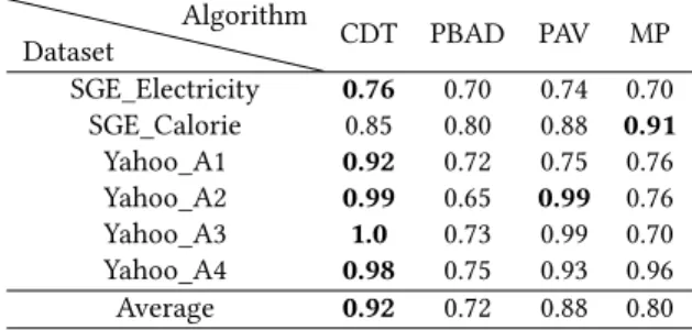
Result Analysis. Table 3 provides the 𝐹 1 score obtained by each algorithm on each of the six univariate time-series datasets. The maximum values of 𝐹 1 score for each dataset are given in bold type. We also calculate the average rank of each method. Table 3: Evaluation of Anomaly Detection using F1-score.

Dataset Algorithm CDT PBAD PAV MP SGE_Electricity 0.76 0.70 0.74 0.70 SGE_Calorie 0.85 0.80 0.88 0.91 Yahoo_A1 0.92 0.72 0.75 0.76 Yahoo_A2 0.99 0.65 0.99 0.76 Yahoo_A3 1.0 0.73 0.99 0.70 Yahoo_A4 0.98 0.75 0.93 0.96 Average 0.92 0.72 0.88 0.80

CDT outperforms the existing baselines in five of the six datasets. It can be observed in Table 3 that our method is more stable for different datasets than baselines. Note that for the competing algorithms, the data should be balanced otherwise, the detection results are poor. We have tested PBAD, PAV and MP on our initial datasets and on a balanced version and we have noticed that its performance highly degrades on the first case. They tend to focus on the accuracy of predictions from the majority class (normal class) which generates poor precision for the minority class (anomaly class).

4.3

Experiments with Rule Learning

Algorithms

We compare our CDT method with the following state-of-the-art rule learning algorithms:

• PART is a combination of C4.5 and RIPPER rule learning to produce rules from partial decision trees using C4.5 algorithm [9].

• JRip implements a rule learner and incremental pruning to produce error reduction (RIPPER) [12]. Rules are formed by greedily adding conditions to the antecedent of a rule. We compare CDT with PART and JRip based on 𝐹 1 score, Q (R) and 𝐹 (ℎ) score (Table 4) and the number of rules produced by the classifiers (Figure 3). We evaluated these methods using WEKA. We use 10-fold cross validation to test and evaluate the PART and JRip with the standard default setting of WEKA. For CDT and each competitor, we use the hyper-parameters values obtained to maximize 𝐹 (ℎ) − 𝑠𝑐𝑜𝑟𝑒 as provided in Table 2.

Result Analysis. Table 4 shows the comparison results for each algorithm in the six datasets using 𝐹 1, Q (R) and 𝐹 (ℎ) score. Note that the results of the F1 score for CDT in Table 4 are different from those in Table 3 because they are not evaluated with the same hyperparameter values (Table 2).

Overall, the average scores show that our approach has got the first position in ranking followed by PART and JRip. CDT outperforms PART and JRip in five of the six datasets in the

𝐹1 score, in three of the six datasets in the Q (R) score and all

datasets in the 𝐹 (ℎ) score. We can observe that the performance of the rule algorithms varies depending on the number of attributes. Typically, with 𝜔 = 31 for the Yahoo_A1 dataset, PART and JRip get a lower 𝐹 1 score, compared with the rest of the datasets. We can observe from the Table 4 that JRip has a high quality of rules Q (R) in three datasets as well as CDT. This is due to the size of its generated rules that are quite short. However, it is less accurate than CDT and PART in almost all datasets. We can also see that none of the baseline algorithms has good 𝐹 (ℎ) overall data sets. While CDT has the best tradeoff between 𝐹 1 score and Q (R) score.

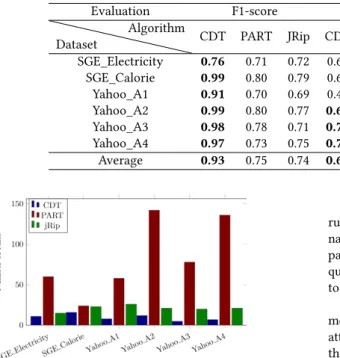
Fig. 3 shows a summary of the number of rules produced by each method. CDT produces a fewer number of rules between 5 and 16 rules. It is followed by JRip that produced reasonably few rules between 15 and 30 rules. However, PART highly produces rules that are between 24 and 142. This is due to the specificity of the rules generated that have low support.

We present some examples of the generated rules by our CDT algorithm from SGE data sets to detect multiple anomalies in Table 5. As we can see, the rules with visualized patterns are easy to intuitively understand and can be easily interpreted by users. The experts give the following comments: the negative peak is considered an anomaly because the energy consumption in a building cannot be negative. The positive peak has occurred

Table 4: Evaluation of anomaly detection using the 𝐹 1 score, the quality measure Q (R) and the objective function 𝐹 (ℎ).

Evaluation F1-score Q (R) F(h)-score

Dataset

Algorithm

CDT PART JRip CDT PART JRip CDT PART JRip

SGE_Electricity 0.76 0.71 0.72 0.67 0.67 0.70 0.51 0.48 0.50 SGE_Calorie 0.99 0.80 0.79 0.61 0.65 0.69 0.60 0.52 0.54 Yahoo_A1 0.91 0.70 0.69 0.48 0.50 0.56 0.43 0.35 0.39 Yahoo_A2 0.99 0.80 0.77 0.69 0.68 0.65 0.68 0.54 0.50 Yahoo_A3 0.98 0.78 0.71 0.77 0.69 0.70 0.75 0.54 0.50 Yahoo_A4 0.97 0.73 0.75 0.70 0.70 0.68 0.68 0.51 0.51 Average 0.93 0.75 0.74 0.65 0.64 0.64 0.61 0.49 0.49

Figure 3: The number of rules generated for anomaly de-tection.

following overconsumption in the building. The collective anom-alies present abnormal variations in successive points. This is due to a fault in the reading of the meters. Finally, the constant anomaly illustrated a stop of the meter.

Table 5: Example of rules generated for anomaly detection in the SGE_Calorie datasets.

5

CONCLUSION

We propose a machine learning method, CDT, that generates human-interpretable rules based on a formalisation of 9 gen-eral patterns of variations for multiple anomaly detection in time-series. The approach is based on a modified decision tree which considers nodes as pattern compositions. Using Bayesian Optimization, we optimized the hyper-parameters such that it maximizes both the rules’quality and the classification perfor-mances. The performance of the presented method was tested using the SGE and Yahoo datasets. Our approach appeared as robust compared to the existing algorithms in conducted experi-ments where their model accuracy decreases in case of multiple anomalies and in generating few interpretable rules.

Future work will concern the improvement of the generated rules. For instance, combine rules by a generalization and elimi-nate redundant rules. Moreover, we could investigate other hyper-parameters such as the size of down-sampling to improve the quality of the generated rules. We could also expand our method to suit multivariate time-series.

Acknowledgment. This PhD. was supported by the Manage-ment and Exploitation Service (SGE) of the Rangueil campus attached to the Rectorate of Toulouse and the research is made in the context of the neOCampus project (Paul Sabatier University, Toulouse).

REFERENCES

[1] Charu C. Aggarwal. 2015. Outlier analysis. In Data mining. Springer, Cham, 237–263.

[2] Nahla Barakat and Joachim Diederich. 2005. Eclectic rule-extraction from support vector machines. International Journal of Computational Intelligence 2, 1 (2005), 59–62.

[3] Sina Däubener, Sebastian Schmitt Hao Wang, Peter Krause, and Thomas Bäck. 2019. Anomaly Detection in Univariate Time Series: An Empirical Comparison of Machine Learning Algorithms. ICDM (2019).

[4] Len Feremans, Vincent Vercruyssen, Boris Cule, Wannes Meert, , and Bart Goethals. 2019. Pattern-based anomaly detection in mixed-type time series. Lecture Notes in Artificial Intelligence (2019).

[5] Zengyou He, Xiaofei Xu, Joshua Zhexue Huang, and Shengchun Deng. 2005. FP-outlier: Frequent pattern based outlier detection. Computer Science and Information Systems 2, 1 (2005), 103–118.

[6] Ines Ben kraiem, André Péninou Faiza Ghozzi, Geoffrey Roman-Jimenez, and Olivier Teste. 2020. Automatic Classification Rules for Anomaly Detection in Time-series. RCIS (2020).

[7] Ines Ben kraiem, André Péninou Faiza Ghozzi, and Olivier Teste. 2019. Pattern-based method for anomaly detection in sensor networks. International Conference on Enterprise Information Systems 1 (jan 2019), 104–113. [8] Nikolay Laptev and Saeed Amizadeh. 2015. A labeled anomaly detection

dataset S5 Yahoo Research, v1. https://webscope.sandbox.yahoo.com/catalog. php?datatype=s&did=70

[9] Daud Nor Ridzuan and Corne David Wolfe. 2009. Human readable rule induction in medical data mining. In Proceedings of the European Computing Conference (vol.1 ed.), Vol. 27 LNEE. 787–798.

[10] Jiang Su and Harry Zhang. 2006. A fast decision tree learning algorithm. In AAAI, Vol. 6. 500–505.

[11] William W.Cohen. 1995. Fast effective rule induction. In Machine learning proceedings 1995. Elsevier, 115–123.

[12] Ian H. Witten and Eibe Frank. 2005. Data Mining: Practical Machine Learning Tools and Techniques (2nd ed.). Morgan Kaufmann.

[13] Hu-Sheng Wu. 2016. A survey of research on anomaly detection for time series. In 2016 13th International Computer Conference on Wavelet Active Media Technology and Information Processing. IEEE, 426–431.

[14] Jia Wu, Xiu-Yun Chen, Hao Zhang, and al. 2019. Hyperparameter Optimization for Machine Learning Models Based on Bayesian Optimization. Journal of Electronic Science and Technology 17 (2019), 26.

[15] Chin-Chia Michael Yeh, Yan Zhu, Liudmila Ulanova, and al. 2016. Matrix profile I: all pairs similarity joins for time series: a unifying view that includes motifs, discords and shapelets. In 2016 IEEE 16th international conference on data mining (ICDM). 1317–1322.

[16] Xiao yun Chen and Yan yan Zhan. 2008. Multi-scale anomaly detection algorithm based on infrequent pattern of time series. J. Comput. Appl. Math. 214, 1 (2008), 227–237.