Compressive Behaviour of Confined Polycrystalline Ice

Publisher’s version / Version de l'éditeur:

Questions? Contact the NRC Publications Archive team at

PublicationsArchive-ArchivesPublications@nrc-cnrc.gc.ca. If you wish to email the authors directly, please see the https://publications-cnrc.canada.ca/fra/droits

L’accès à ce site Web et l’utilisation de son contenu sont assujettis aux conditions présentées dans le site LISEZ CES CONDITIONS ATTENTIVEMENT AVANT D’UTILISER CE SITE WEB.

PERD/CHC Report, 2001-12

READ THESE TERMS AND CONDITIONS CAREFULLY BEFORE USING THIS WEBSITE. https://nrc-publications.canada.ca/eng/copyright

NRC Publications Archive Record / Notice des Archives des publications du CNRC :

https://nrc-publications.canada.ca/eng/view/object/?id=272a2135-1cae-485a-b3d2-07086fdee6a5 https://publications-cnrc.canada.ca/fra/voir/objet/?id=272a2135-1cae-485a-b3d2-07086fdee6a5

Archives des publications du CNRC

For the publisher’s version, please access the DOI link below./ Pour consulter la version de l’éditeur, utilisez le lien DOI ci-dessous.

https://doi.org/10.4224/12340921

Access and use of this website and the material on it are subject to the Terms and Conditions set forth at Compressive Behaviour of Confined Polycrystalline Ice

Compressive Behaviour

Of Confined Polycrystalline Ice

Report prepared for

The National Research Council

Program on Energy Research and Development (PERD)

By

Paul D. Barrette and Ian J. Jordaan

Ocean Engineering Research Centre

Memorial University of Newfoundland

St. John's, NF

December 2001

Table of Content

Table of Content 2

Acknowledgements 4

1. Introduction 5

2. Purpose and Methodology 6

3. General Notions and Principles 7

3.1. Stress 7

3.2. Strain 10

3.3. Type of Tests 10

3.3.1. Creep test 11

3.3.2. Constant Strain-Rate Test 11

3.3.3. This study 11

3.4. Constitutive modeling 12

3.4.1. Elasticity 13

3.4.2. Visco-Elasticity 15

3.4.3. Plasticity 15

3.5. The Rheology of Ice 16

3.5.1. Phenomenology 16

3.6. Temperature 16

3.6.1. Basic Concept 16

3.6.2. Physics of ice behaviour near its melting point 19 3.6.3. Temperature considerations in triaxial testing 21

4. Previous work 22

4.1. Effects of confining pressure 23

4.2. Temperature and activation energy 24

5. Testing and Results 28

5.1. Rationale 28

5.2. Laboratory Procedures 29

5.2.1. Production of ice specimens 29

5.2.2. Density and grain size 29

5.2.3. Testing 30

5.3. Results 30

5.3.1. Overview of testing 30

5.3.2. Minimum strain rate and activation energy 32

6. Summary 35

7. Implications for ice-structure interactions 35

Appendix 1 Previous investigations on the triaxial testing of ice 44

Appendix 2 Photography of ice specimens and internal structure 51

Acknowledgements

The experimental work presented in this report was done with the assistance of several COOP work-term students registered in the Engineering program of Memorial University of Newfoundland. These are: Amanda Bromley, Sterling Parsons, Paul Garnier and Thomas Mackey. Ron O’Driscoll and Austin Bursey, both technicians at the Faculty of Engineering and Applied Science, looked after the maintenance of the cold room refrigeration unit and the MTS hydraulic system. Austin Bugden, technical officer with the Institute for Marine Dynamics (IMD) of the National Research Council of Canada in St.John’s, endeavoured to accommodate our needs for the IMD cold room facility and its ice machining and thin sectioning equipment.

Dr. Irene Meglis collaborated with the data production in the early stages of the project. She was instrumental in gathering an initial database. Both Dr. Meglis and Paul Melanson provided useful guidance in initiating the ice production procedure and setting up the MTS system to resume ice testing.

Dr. Stephen Jones allowed us access to IMD and the logistical support that was necessary to carry out the research presented in this report. Dr. Jones also made his expertise available in a number of discussions on the interpretation of the data.

1. Introduction

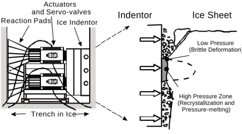
The design of structures and vessels for arctic and subarctic waters requires knowledge of ice loads and their distribution in space and time. This in turn requires analyses of the interaction between the structure and the ice at conditions that are representative of the real scale event (displacement rate, confining pressure, deviatoric stress, temperature). Medium-scale field investigations have been carried out in the past in an effort to better comprehend the failure processes in the ice during these interactions. An example of this are a series of indentation tests that have been conducted with iceberg and multiyear ice (Frederking et al. 1990, Masterson et al. 1992, 1999). A test set- up is shown in Figure 1.

Ice Sheet Indentor

High Pressure Zone (Recrystallization and Pressure-melting) Low Pressure (Brittle Deformation) Ice Indentor Reaction Pads Actuators and Servo-valves Trench in Ice

Figure 1: Medium-scale field testing experiments.

Indentors of various shapes were used. Loads, displacements and temperature are some of the parameters that were recorded during these tests. The actuator response typically displayed a saw-tooth loading pattern that was explained by the dynamics of the failure processes occurring in the ice. Local pressures along the interface between the ice and the structure reach relatively high levels (up to 70 MPa, according to Frederking et al. 1990). Our analyses of the medium-scale field events produced with either iceberg or multiyear ice has outlined non-simultaneous failure modes and the occurrence of high pressure zones that effectively control the load applied onto the structure (Jordaan et al. 1999, 2001)(Fig. 1). Mechanisms of a ductile nature, such as recrystallization, have been shown to occur in these zones (Muggeridge and Jordaan 1999). The brittle behaviour and spalling accompanying ice failure are closely associated with what is happening inside the high pressure zones. An adequate representation of the deformation mechanisms occurring in the ice during mechanical testing therefore requires high confinement levels. Triaxial testing was done by a number of investigators. Amongst the most interesting observations made in some of these studies is an increase followed by a decrease in strength of the material with an increase in confinement, particularly at high strain rates

(Jones 1978, 1982, Nadreau and Michel 1986, Richter-Menge 1991, Mizuno 1998). A decrease followed by an increase of 'compliance' with an increase in confinement was also reported in constant load tests (Jones and Chew 1983, Melanson et al. 1999a, Barrette and Jordaan 2001). This reversal in trend, if representative of what is taking place during a real ice-structure interaction, is significant for two reasons:

First, it indicates that high-pressure zones may become 'softer' where pressure is highest, thereby exerting some control on the failure mode of these zones and the resulting load-unloading cycles.

Second, the reason for this reversal was attributed to recrystallization phenomena and the pressure melting of ice. Evidence of these mechanisms was provided (Frederking et al. 1990, Gagnon and Molgaard 1991). If this is the case, what was previously interpreted as pristine, undeformed ice at the ice- indentor interface after unloading (so-called 'blue zones') may have been strongly deformed - or structurally 'damaged' - ice. Highly recrystallized ice is translucent, and no evidence of its deformation would be noticeable from video monitoring.

Another issue that could benefit from further investigation is the effect of loading on the temperature of the ice. A rise in temperature is expected upon the application of high axial stress. This rise corresponds to a release in thermal energy as a response to loading, with the possible contribution of frictional heating as the ice deforms. At high hydrostatic levels, which decrease the melting point of ice, this temperature rise may be sufficient to bring the ice, at least locally, to its melting point. The latent heat of fusion absorbed from the surrounding ice as a result of melting should contribute to a decrease in temperature.

2. Purpose and Methodology

The main objectives of the research presented in this report are three-fold:

• To investigate the effect of hydrostatic pressure on the deformational behaviour of ice specimens produced in the laboratory.

• To investigate the effect of temperature on the deformational behaviour of these specimens and provide an estimate of the activation energy for the deformation at various confinement levels.

• To establish a comparative basis between the deformational behaviour of laboratory-produced ice and naturally formed ice of glacial origin.

Other themes of interest include:

• The effect of loading on the thermal behaviour of the ice.

Research on these other themes is on going as of this writing and will be reported elsewhere.

We begin with a section describing some of the basic notions related with triaxial deformation, the rheology of ice and the concept of 'temperature'. This is an attempt to make the text somewhat self-explanatory in terms of the approach, terminology and background relevant to the later sections. A review of the existing literature on the triaxial testing of ice is then provided. This is followed by a description of the experimental procedures, the results and a discussion. Appendix 1 encloses a detailed account of previous investigations. Appendix 2 provides photographs of various features related with the test specimens and their internal structure. The data is in Appendix 3.

3. General Notions and Principles

Stress is a force normalized over an area. It is a second-order tensor, which means that it has two free indices: its magnitude depends on both the orientation of the force and that of the surface on which it acts. This is usually represented as follows:

          = 33 23 13 23 22 12 13 12 11 σ σ σ σ σ σ σ σ σ σij _{Eq. 1}

The stress conditions that are simulated with ice specimens in the laboratory are those corresponding to the equation below (whereby σij = 0) because they are simpler to obtain: only the three principal stresses (σ11, σ22 and σ33) need to be controlled.

          = 33 22 11 0 0 0 0 0 0 σ σ σ σij _{Eq. 2}

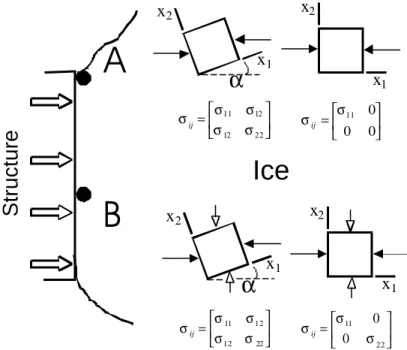
It is also more representative of the stress acting on a free body element when one of its reference axes is parallel to the direction in which the load is applied onto the ice (this point is illustrated in Figure 2 for a two-dimensional case).

A uniaxial stress is one in which one principal stress, either σ1 (for a compressive stress)

or σ3 (for a tensile stress), is non-zero and the other two are equal to zero. Uniaxial testing

may be done, for instance, to study the mechanical behaviour of the ice near one of its free surfaces (location A in Figure 2). A biaxial stress is one in which two of the three principal stresses are nonzero and the third one is zero. A triaxial state of stress is one in which all three principal stresses are non- zero. This will generally be the case in an ice

Ice

Structure

A

B

α

α

Figure 2: The stress at a point, represented by a free body element, and equivalent stress tensors for two different locations along the ice-structure interface. The reference axes to the left are at an angle α with the compression direction of the indentor, and σij ≠ 0. To the right, the references axes are chosen so that

one axis is parallel to the compression direction, and σij = 0.

Near a free surface (location A), only the compressive forces from the indentor and their reaction (black arrowheads) will act on the ice. Away from the free surfaces (location B), the ice exerts a confinement (white arrowheads).

Figure 3: Loading regime on an ice specimen. The white and black arrows symbolize the confinement and axial compressive load, respectively.

body, except at locations very near the free surfaces. The reason for this is that, elsewhere, the ice exerts a given level of confinement during the deformation, which will increase with distance away from the free surfaces (location B in Figure 2).

The stresses to which ice may be submitted and the deformation that results from it are divided into two fundamentally distinct states. The first one involves a change in volume, whereby the crystal lattice remains intact but the constituents' atoms and molecules are forced either closer together (contraction) or farther apart (dilation). The stress causing this condition is referred to as hydrostatic (or isotropic) and leads to a deformation that is elastically recoverable. The second state involves a distortion in the crystal lattice and ultimately leads to a permanent change in shape due to the break up of atomic bonds. This is known as a deviatoric stress. It is the deviatoric component that causes the material to fail or yield, either in a brittle fashion, through the formation and propagation of cracks, or in a ductile fashion, through recrystallization and other processes.

The total stress is the summation of the hydrostatic and deviatoric components:

          − − − +           =           ) ( ) ( ) ( 0 0 0 0 0 0 33 23 13 23 22 12 13 12 11 33 23 13 23 22 12 13 12 11 p p p p p p σ σ σ σ σ σ σ σ σ σ σ σ σ σ σ σ σ σ Eq. 3

where p is the hydrostatic pressure, also called mean stress, and given by:

3

) (σ₁₁ +σ₂₂ +σ₃₃ =

p _{Eq. 4}

This equation is a generalized form for the stress conditions that may exist at a given location inside the ice body. As mentioned earlier, we are able to simplify this situation by considering an equivalent set of stress conditions with the three mutually perpendicular planes along which all σij stresses are zero. Thus,

          − − − +           =           ) ( 0 0 0 ) ( 0 0 0 ) ( 0 0 0 0 0 0 0 0 0 0 0 0 33 22 11 33 22 11 p p p p p p σ σ σ σ σ σ Eq. 5

This represents the stress existing inside the ice body when one of the reference axes (σ11) is parallel to the direction of relative motion between the ice and the indentor. It is possible to obtain a basic reproduction of this stress regime by conducting triaxial tests, involving the superposition of a confinement and a uniaxial stress. The equipment we used for our investigations allows us an independent control over these two stresses. The first one is obtained by compressing the oil in which the ice specimen is immersed. The second one is obtained by loading the specimen axially. This is shown schematically

in Figure 3. For example, if we were to submit an ice specimen to a 50 MPa confinement (white arrows) and a 15 MPa axial compression (black arrows), the stress along the compressive axis (σ1) would be equal to the summation of both stresses - corresponding

to 65 MPa. The stresses along the other two axes (σ2 and σ3) would both be 50 MPa. The

hydrostatic stress is then 55 MPa. The deviatoric stresses are as 10, -5 and -5 MPa, respectively, for σ1, σ2 and σ3.

3.2. Strain

Strain is a measure of deformation. In a specimen, it is expressed as a difference between the original (L0) and deformed (L) length of a material line (which, for small increments, may be represented by dL). The engineering strain is the deformation normalized over the original length:

0 0 ) ( L L L E − = ε _or 0 L dL dεE = _{Eq. 6}

The total, or true, strain can be obtained by integration:

[

]

∫

With increasing deformation, the true strain becomes progressively larger than the engineering strain. The use of the true strain is more appropriate when deformation exceeds a few percent.

Strain is also a second-order tensor. The strain tensor can be resolved into an isotropic and a deviatoric component:

          − − − +           =           ) ( ) ( ) ( 0 0 0 0 0 0 33 23 13 23 22 12 13 12 11 33 23 13 23 22 12 13 12 11 H H H H H H ε ε ε ε ε ε ε ε ε ε ε ε ε ε ε ε ε ε ε ε ε ε ε ε Eq. 8

where εH is the isotropic strain:

3

) (ε₁₁ ε₂₂ ε₃₃

εH = + + _{Eq. 9}

3.3.1. Creep test

The word creep is often used to describe time-dependant deformation under any loading regime. A more rigorous definition is when a constant stress is applied to a specimen, which then undergoes a progressive deformation with time (e.g. Popov 1990). In most cases, the area through which the load is transmitted either increases (in compression) or decreases (tension) as the specimen deforms, so that the stress is only nominally constant under constant load. Because time-dependant deformation mechanisms (related with the motion of crystal defects) are thermally-activated, creep tests can only be done at a temperature that is close to the melting point of the material, as is the case for most ice engineering applications. Creep will occur at lower temperatures but at a time scale that is too long to be practical for testing and that may not be relevant to engineering.

3.3.2. Constant Strain-Rate Test

In this case, the force applied onto the specimen varies to maintain a constant strain-rate. This test is often referred to as a strength test, because it records the stress at which the material yields. The relative displacement of the platens is hydraulically-controlled by a closed- loop feedback from displacement gages that are attached directly onto the specimen. This allows the compliance of the testing system to be excluded from the measurements (Sinha 1979a, 1981a,b). With this method, only the deformation at the centre of the specimen is considered, leaving out that occurring near the platens, which is non uniform due to the boundary conditions. Constant strain rate tests are usually more popular in the ice engineering community because they provide numbers on the strength of ice and its strain-rate sensitivity.

3.3.3. This study

Only creep testing was done as part of this study. The reason was that our investigations were originally designed to be an extens ion of an earlier testing program in which specimens were submitted to a constant load (Meglis et al. 1999, Melanson et al. 1999a). Another reason is the technical challenge related with the use of displacement gages attached onto the ice specimens: the la tter were enclosed in a latex jacket to prevent penetration of the confinement fluid during deformation. Also, large strains were achieved in our tests, leading to a substantial change in specimen morphology and the resulting difficulty in maintaining the gages in position. The strain in the specimen could therefore only be measured by monitoring the displacement between the platens.

A correspondence between constant strain rate and constant load tests was established by Mellor and Cole (1982, 1983) and Sinha et al. (1995). They have shown that, when properly interpreted, creep curves can also provide information on the failure strength. The ultimate yield strength in this type of tests is the equivalent to the minimum strain rate for a material submitted to a constant stress. This means that if a constant strain rate test, done with a strain rate X, results in a strength Y, the same material submitted to a constant stress Y should display a minimum strain rate of X (Figure 4).

The minimum strain rate is a useful index: it allows to monitor the relative ‘compliance’ of the material under different loading conditions. The higher the minimum strain rate the

Ultimate Yield Strength

Minimum Strain Rate

Stress

Figure 4: Response of ice when it is submitted to 1) a constant stress (for which the strain rate is recorded) and 2) a constant strain rate (for which the stress is recorded). The minimum strain rate in the former is equivalent to the ultimate strength in the latter.

more compliant is the ice. On the basis of the aforementioned correspondence, we would expect the ultimate yield strength of the ice to decrease with the same change in loading conditions.

3.4. Constitutive modeling

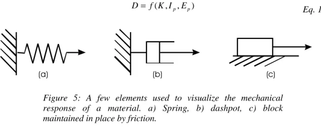
The rheological behaviour of a material is specified by the relationship between dyna mic (stress) and kinematic (strain) quantities. Constitutive modeling is a mathematical expression of this behaviour. The relationship also involves intrinsic (material properties such as mass, elastic properties, viscosity,...) and extrinsic (time, temperature, pressure, ...) parameters. Newton's Second law of Motion F=ma is an example, relating a dynamic (force F) and a kinematic (acceleration a) quantity, with an intrinsic material parameter (mass m). A more general form of this relationship may be

) , , (K Ip Ep f D= _{Eq. 10} (a) (b) (c)

Figure 5: A few elements used to visualize the mechanical response of a material. a) Spring, b) dashpot, c) block

where D represents the dynamic quantity (force, stress, stress rate, ...), K represents the kinematic quantities (displacement, velocity, strain, strain rate,...), and Ip and Ep are the intrinsic and extrinsic parameters, respectively.

One of the main purposes of experimental work is to provide information on the nature of that relationship.

A classification scheme has been devised in continuum mechanics to represent a number of rheological behaviours. This scheme uses conceptual elements, including a spring, a dashpot and a body resting on a surface and maintained in place by friction (Figure 5).

(a)

(b)

(c)

Figure 6: Three common type of rheological behaviours. a) Elastic, b) visco-elastic, c) plastic.

These are combined in a variety of ways to generate a stress-strain behaviour, also known as phenomenological behaviour, that compare with the actual response of the material to given loading conditions. The spring on its own reproduces the elastic response; a combination of a spring and a dashpot represents visco-elasticity; and a combination of a spring and a body in frictional contact with the surface corresponds to plasticity (Figure 6).

3.4.1. Elasticity

Elasticity is a phenomenon that can be linked directly with the structural nature of the material: it is the macroscopic expression of the electro- magnetic forces that keep individual atoms at an 'equilibrium' distance from each other. This is the reason why

elastic deformation is reversible. The magnitude of these forces depend on the length of the bond, and how it is defined: in general, covalent bonds are stronger than metallic bonds, which are in turn stronger than ionic bonds. Temperature affects the length of the bonds and this will be discussed later. Most materials behave elastically under small

ε

σ

time

time

t

t

(a)

(b)

(c)

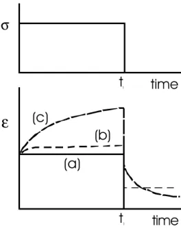
Figure 7: Rheological behaviours on a strain-time diagram, upon the application of a stress. a) elastic, b) visco-elastic, c) plastic.

loads. Both the deformation and recovery are time- independent (Figure 7). The stress-strain behaviour is linear and is described by Hooke's law (σ=Eε shown in Figure 8a ). This relationship is usually applied to a change in length. The material constant E, also called Young's modulus, may be replaced by a shear modulus to describe the elasticity of shape, or by a bulk modulus to describe the volume elasticity.

σ

σ

σ

ε

E µ µ

ε

ε

(a) (b) (c)

Figure 8: Rheological behaviour corresponding to a) elasticity, b) linear visco-elasticity and c) non linear visco-elasticity. Note that that stress is plotted against strain rate in (b) and (c).

3.4.2. Visco-Elasticity

Once the elastic limit is reached, visco-elastic materials display a gradual increase in strain but at a decreasing strain rate. Stress removal at time t1 leads to the instantaneous elastic recovery, followed by a time-dependant or 'delayed' elastic component (Figure 9). In terms of the mechanical response to loading, ice is best described as a visco-elastic material. The establishment of a physical basis for visco-elasticity is more complex than in the case of elasticity. They are tied in not only with the bonding energy but also with generation and motion of crystal defects (dislocations, vacancies, diffusion-related phenomena, ...) and, depending on the external parameters such as pressure and temperature, the formation of microcracks. Mechanisms accounting for this type of behaviour must also involve grain boundaries. Indeed, the deformation of single ice crystals has been shown to differ significantly from polycrystalline ice. Firstly, the elastic response is followed by accelerating instead of decelerating creep1. Secondly, the creep of single crystals does not display a delayed elastic component.

Viscosity may be expressed as

µ σ ε& = n

Eq. 11

where ε· is the strain rate, σ is the stress and µ is the viscosity. For linear visco-elastic solids (also known as Newtonian), n =1 and the material behaves like a liquid2. For non-linear visco-elastic solids, n > 1.

3.4.3. Plasticity

Plasticity often designates the deformation occurring after the elastic limit is reached (that is, when the force applied to the material is high enough to overcome the strength of the atomic bonds). The word anelasticity is also used as for that purpose. The ice response to loading is thus commonly referred to as plastic in the engineering literature. A more rigorous usage of the term plasticity implies a particular behaviour of the strain once the elastic limit is exceeded: the strain increases a little more before stabilizing to a constant

1

Accelerating and decelerating creep are discussed later.

2

The notion that a solid substance may flow like a liquid may be better understood by considering the Deborah number D. This is the ratio of the time required for a measurable amount of creep over the time during which the observation is done and limited to the life expectancy of the observer. If D is small, we perceive the material as a liquid. If D is large, it is seen as a solid. In both cases, there is linear relationship between ε· and σ (which is characteristic of what we acknowledge as a liquid on an every day basis).

value. The elastic deformation is recovered upon the removal of the stress, and a permanent strain remains, without a delayed elastic component. Plasticity does not describe the phenomenological response of ice. The concept of visco-elasticity is preferred for this purpose.

3.5. The Rheology of Ice 3.5.1. Phenomenology

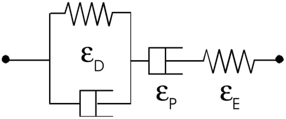
Figure 9 is a typical creep response of polycrystalline ice observed during our investigations. This behaviour is often represented conceptually by Figure 10. The delayed elasticity is simulated by a combination of a dashpot and a spring arranged in parallel, referred to as a Kelvin unit. The combination of a dashpot (viscous strain) and a spring (elastic strain) arranged in series is known as a Maxwell unit. The entire assembly is called a Burgers' model and is the one that is most commonly used to express the creep of ice. The total strain εT is therefore

P D E

T ε ε ε

ε = + + _{Eq. 12}

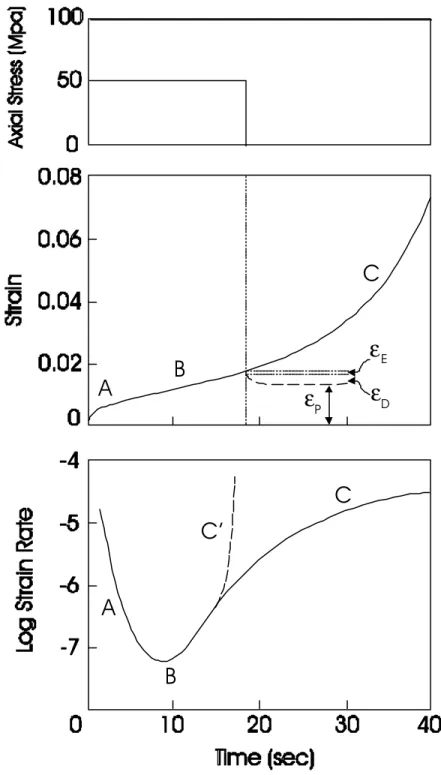
The elastic deformation εE in a standard creep test is a very small portion of the total deformation (typically 0.1 to 0.5% strain, depending on loading rate). It is therefore not a significant issue in this study, particularly if we focus on very high strains. The delayed elastic deformation εD has been attributed to grain boundary sliding (Sinha 1979b, 1984a). This phenomenon takes place immediately after the elastic strain and is also a relatively small part of the total deformation. It induces a decelerating phase in the early part of the deformation (A in Figure 9). The permanent strain εP is the deformation that results from the generation of microcracks and/or the motion of crystal defects. These mechanisms begin as soon as the load is applied but their contribution to the total deformation is initially negligible. It becomes more important as the deformation rate reaches a minimum (B) and begins to accelerate (C).

The terms 'primary', 'secondary' and 'tertiary' creep is used consistently in the ice literature to designate stages A, B and C in Figure 9. This usage has an historical basis: it was borrowed from metallurgical studies, in which metals and alloys undergoing creep spend most of their design life span in the secondary stage. This is not the case for ice, where the secondary creep is no more than an inflexion point between a decelerating and an accelerating phase. This terminology is therefore not retained in the present report.

3.6. Temperature

3.6.1. Basic Concept

Physically, temperature is the amount of kinetic energy, or heat, stored by the individual atoms making up a given substance (gas, liquid or solid). This energy corresponds to a large extent to the vibration of the atoms about their equilibrium position. The melting

ε

ε

ε

A

A

B

B

C

C’

C

Figure 9: Creep response for freshwater, polycrystalline ice at 55 MPa hydrostatic pressure, 15 MPa axial stress and a temperature of -10oC. The elastic (εE), delayed elastic(εD) and

permanent (εP) component of the deformation are best seen upon

unloading the specimen. A: Decelerating creep, B: Minimum creep rate, C: Accelerating creep, C': Run-away behaviour.

ε

ε

_P

_E

ε

_D

Figure 10: Behaviour of polycrystalline ice, shown by a combination of springs and dash-pots.

point of a crystalline substance is reached when the amplitude of the vibrations is such that it is able to overcome the molecular bonding energy. Substance with weaker bonds will have a lower melting point. Absolute zero on the Kelvin temperature scale (-273oC) is a theoretical value at which atomic vibrations in all substances cease to exist. At that temperature, matter becomes inert and one may envisage air molecules lying on the ground, no longer able to surmount gravitational attraction.

A consequence of the Second Law of Thermodynamics is that energy spontaneously tends to flow only from where it is concentrated to where it is diffused. Consequently, it spreads out. In some cases, such as the cooling down of a frying pan when it is taken off the kitchen stove, this phenomenon will take place instantaneously. But there are other cases where it will not because of the existence of molecular bonding. This applies, for instance, to any form of fuels. Wood or coal will react with oxygen to form CO2 and

H2O, which have a lower energy configuration. The difference in energy is dissipated in

the form of 'heat'. But this reaction will only occur if the energy barrier, called activation

energy and represented by molecular bonding in the reactants, is overcome. (This can be

done quite effectively, in the case of a liquid fuel, with a lighted match.) The determination of the activation energy will be addressed in this report as it is a useful indication of what mechanism controls the deformation of the material.

-8 -4 0 4 8 12 16

Temperature (deg. C)

Density (g/ml)

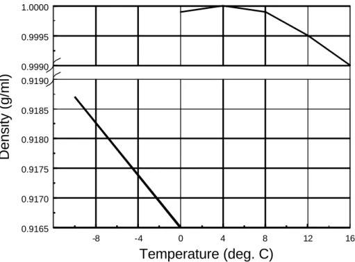
Figure 11: Density variation of ice and water across the phase transition. The data is from Bolz and Tuve (1970) and Hobbs (1974).

3.6.2. Physics of ice behaviour near its melting point

The oxygen atom in a H2O molecule is more electronegative than the hydrogen atom, and

the resulting H-O bonds have a 39% ionic character (Metcalfe et al. 1974). Consequently, the electrons are on average concentrated around the oxygen nucleus. Since the covalent bonds of the water molecule do not line up (the angle between the two bonds is about 105o), it has a polar character. This polarity causes water molecules to be attracted to each other, thus defining the weaker hydrogen bond. In the solid phase (ice), H2O

molecules are arranged in a hexagonal crystal structure.

Above absolute zero (0oK), the atoms making up the ice structure (or any other crystalline substances) vibrate. They do so anharmonically (out of phase), so that an increase in temperature induces an increase in volume, and a consequent reduction in density (Figure 11). As temperature increases, the bonds are stretched further and begin to break, the macroscopic expression of which is referred to as melting. Since the hexagonal crystal structure of ice is known to be very open, the water molecules can easily fit inside this structure once the bonds are broken. Doing so, they take up less space than when they were part of the crystal structure, which accounts for the increase in density across the phase change (Figure 11). The density then increases again slightly in

the liquid phase to a maximum of 1.0000 g/ml at 4oC, before dropping again. This is explained by the occurrence of two competing phenomena: 1) The on-going breaking down of the hydrogen bonds allows the water molecules to get closer together; 2) The increase in thermal energy overcomes the polar attraction between water molecules (Metcalfe et al. 1974). The first mechanism predominates only up to 4oC.

According to the Clapeyron equation,

(

)

where Tm is the melting temperature of ice in degrees Kelvin, p is pressure, Lf is the latent heat of melting per unit mass and vi and vw are the specific volume of ice and water, respectively. For ice, A = 0.0743oC / MPa at 0oC and 0.0833 oC / MPa at -10oC. At a pressure of 70 MPa, the ice specimen would be expected to melt at about 5.5oC. At a temperature of -10oC, melting occurs at 120 MPa. This is a direct consequence of the fact that ice expands upon freezing. A close examination of the following equation, derived from the one above, will help better understand this phenomenon:

) ( ) ( i w i w m e e v v dp dT − − = _{Eq. 14}

where ew and ei are the entropy of water and ice, respectively. The denominator of the right- hand term will necessarily be positive since entropy, which is the amount of disorder, is always higher in the liquid than it is in the solid. In the hypothetical case where the change of phase would not be accompanied by a change in volume, the melting point would not be affected by pressure (A = 0). Other materials that contract upon melting include Pu, Ge, Si, Bi, Sb and Ga (Poirier 1985). For most materials, however, the solid to liquid transition causes an increase in volume. If this phase change occurs when the material is at a high pressure, more energy will be required to compensate for the additional work exerted on the system by that pressure. This means melting will take place at a higher temperature. The opposite holds for ice since it looses volume upon melting (Figure 11).

Another outstanding feature with ice is its comparatively high degree of brittleness even when it is near or at its melting point. Most other crystalline substances will behave like soft putty near their melting temperature. The reasons for this unusual behaviour is tied in with a very low dislocation mobility and a high stability of its lattice structure, the latter resulting in a low solid solubility of vacancies and impurities (Barnes et al. 1971).

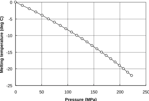
-25 -20 -15 -10 -5 0 0 50 100 150 200 250 Pressure (MPa)

Melting temperature (deg C)

Figure 12: Variation of the melting temperature of ice with pressure (Nordell 1990).

3.6.3. Temperature considerations in triaxial testing

For the purpose of the following discussion, the system refers to what is enclosed in the triaxial cell (the ice specimen and the confining oil). According to the First Law of Thermodynamics, the change in the internal energy of this system (∆U) is equal to the

thermal energy Q transferred to the system minus the work W done by the system on its surroundings:

W Q U = −

∆ _{Eq. 15}

Q is negative when the thermal energy is transferred from the system. Similarly, W is

negative if the work is done on the system. In the case of ice specimens, the internal energy is represented mostly by the thermal energy (the kinetic energy of the atoms) and the strain energy (the elastic energy stored in the crystal lattice). Other forms of internal energy, such as nuclear energy and chemical energy, can here be neglected. If we assume that the system is thermally isolated, or adiabatic, then there is no heat transfer in or out of the system (Q = 0). Thus ∆U = -W. This situation roughly approximates our triaxial

test conditions1. The work W is represented either by an increase in confinement and/or

1

The triaxial cell we used is made out of steel so it is far from being thermally insulated. But heat transfer across the wall of the cell is relatively slow and is therefore neglected for the purpose of this discussion.

the application of an axial load. Either way, it is negative, leading to an increase in internal energy.

One question that is of interest concerns the amount of thermal energy absorbed by the ice during testing. Only 5 to 10% of the energy applied onto a any given specimen is stored in the defect structure (Nemat-Nasser 2000, p. 431). This implies a significant departure from isothermal conditions. If heat flow takes place (in the case the deformation is not entirely adiabatic), either by conduction through the end platens or the confining oil, this will lead to a non- uniform temperature distribution in the deforming specimen. This is an issue that has not attracted a lot of attention from the ice engineering community. Its relevance lies in the fact that the compressive strength of ice is a function of its temperature.

4. Previous work

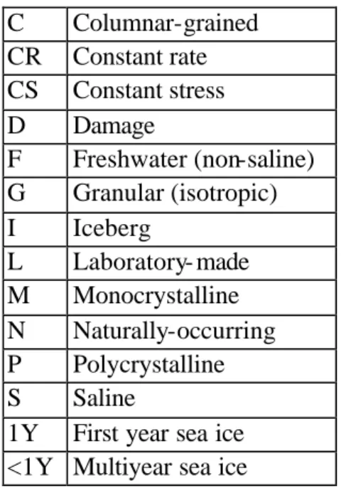
A survey of the open literature reporting triaxial test data on various types of ice was carried out as part of our investigations. Fifty papers, published between 1958 and 2001 inclusively, were retrieved (Barrette 2001). This compilation only considers papers enclosing triaxial test data, and leaves out numerical and theoretical treatments. Testing under biaxial stress or plane strain conditions (e.g. Frederking 1977, Sinha 1984b, Timco and Frederking 1986) was therefore not included. Investigations on the elastic properties of ice under confinement were not searched either. The reader is referred to Gagnon et al. (1988) for this topic. Moreover, all of the data encountered were obtained from the hexagonal polymorph of ice (Ih) with few exceptions (e.g. Kirby et al. 1985, Durham et al. 1996). These were also omitted. Finally, only the English literature was surveyed. The results of our search is presented in Appendix 1 (the abbreviations used in this appendix are explained in Table 1).

Both artificial and naturally-occurring ice types were investigated. The control on the deviator was generally done in two ways. Constant strain rate tests are those for which either specimen deformation or the rate of relative displacement between the upper and lower platen was kept constant. Constant stress - or creep - tests were also used. The stress was usually nominal since few investigators (e.g. Jones 1978, Mizuno 1992, Melanson et al. 1999a) reported a correction to compensate for a change in specimen area (required especially when large strains are achieved). All confined testing was done with a compressive axial stress, with the exception of Rigsby (1958)(shear) and Haynes (1973) (tension). In a few cases, a damage mechanics approach, instead of conventional visco-elasticity, was applied to the behaviour of ice to acknowledge the effect of load history on further incremental deformation (e.g. Jordaan and collaborators). Maximum axial stress is indicated for constant load tests; the logarithm of strain rate is indicated for constant

Table 1: List of abbreviations used in Appendix 1. C Columnar-grained CR Constant rate CS Constant stress D Damage F Freshwater (non-saline) G Granular (isotropic) I Iceberg L Laboratory- made M Monocrystalline N Naturally-occurring P Polycrystalline S Saline

1Y First year sea ice <1Y Multiyear sea ice

strain rate tests. The temperature range of the test series is also indicated, along with the salient results.

Specimen confinement was usually delivered by a hydraulic fluid. In some cases, a constant ratio between axial and confinement stresses was maintained throughout the deformation. True multiaxial testing with brush-type platens, whereby loading along all axes of three-dimensional space is controlled independently, was also conducted. For these cases, no maximum confinement is shown in the results of our search. Discussions on the use of brush platens and multiaxial testing may be found in Haüsler (1981), Schulson et al. (1989), Haüsler et al. (1991) and Melton and Schulson (1998a). Following is a summary of these findings.

4.1. Effects of confining pressure

There is a general consensus that an increase in hydrostatic (or confinement) pressure causes an increase in the strength of freshwater (non saline) ice for constant strain rate experiments (Jones 1982, Mizuno 1998, Rist et al. 1988, 1994, Kalifa et al. 1989, 1992, Murrell et al. 1991, Nadreau et al. 1991) and a decrease in minimum strain rate for creep testing (Golubov et al. 1990, Jones and Chew 1983, Barrette and Jordaan 2001). This increase in 'compliance' has been observed at various creep loads and temperatures. It was also documented for natural or artificial sea ice (Nawar et al. 1983, Blair 1988, Cox and Richter-Menge 1988, Golubov et al. 1990, Sammonds et al. 1998, Rist. and Murrell 1994) and genuine iceberg ice (Nadreau and Michel 1986, Gagnon and Gammon 1995).

For strength tests, an increase in strain rate caused a steeper increase in the maximum deviator, following which the strength tend to level off.

A reversal in this trend was documented in studies that were able to investigate the deformational behaviour of ice at levels of hydrostatic or confinement pressures extending beyond 30 to 50 MPa. This was shown in constant strain rate tests, where the strength (or maximum deviator) reached a peak value between 10 and 50 MPa pressure (Durham et al. 1983, Kirby et al. 1985, Nadreau and Michel 1986, Richter-Menge 1991). A reversal was also documented with creep tests, whereby the minimum strain rate decreased with increasing pressure, then increased with further increase in pressure (Jones and Chew 1983, Barrette and Jordaan 2001). Furthermore, Jordaan and collaborators (see Jordaan et al. 1999, 2001) devised a formulation for the rate of damage in the accelerated zone of the creep curve. This rate was found to decrease up to hydrostatic pressure 30-40 MPa, and increase upon further pressure increase (Melanson et al. 1999a).

This reversal, or 'pressure softening effect', is generally attributed to the fact that, upon increasing pressure, the ice gets closer to its melting temperature. Locally, it may undergo melting, perhaps at specific locations along grain boundaries where stress cannot be readily accommodated by dislocation or diffusion-controlled deformation mechanisms. To the authors' knowledge no direct evidence of this phenomenon was presented to date. What may be stated is that an increase in pressure is thermodynamically equivalent to an increase in temperature. A better approach in the study of temperature effects may be to consider the temperature difference with respect to melting point, as opposed to the actual temperature at which testing takes place (Rigsby 1958).

4.2. Temperature and activation energy

An increase in temperature is known to cause a decrease in strength in constant strain rate experiments and an increase in strain rate for constant loading (Mellor and Testa 1969, Mellor 1980). This is also observed in specimens under triaxial pressure conditions (Durham et al. 1983, Cox and Richter-Menge 1988, Gagnon and Gammon 1995). This phenomenon is readily understood if one considers that a higher temperature induces an increase in the amount of kinetic energy within the material. Molecular bonding is therefore more easily overcome when submitted to addit ional energy in the form of mechanical stress.

The most commonly used formulation for the determination of activation energy follows the usual Arrhenius relationship:

) exp( min RT Q − ∝ ε& _{Eq. 16}

used instead of R, depending on which units are used for energy. In some cases, Q is the activation enthalpy, and is defined as

PV E

Q= + _{Eq. 17}

where E is the activation energy, P is the pressure and V is the activation volume (e.g. Jones and Chew 1983, Durham et al. 1983, Mizuno 1992).

Taking the natural logarithm on both side of the Arrhenius relationship,

) ( ) ln( RT Q f − = ε& _{Eq. 18}

Q can be determined from a plot relating the logarithm of strain rate and 1/T. For creep

tests, the minimum strain rate is considered for this exercise. For constant strain rate test, it is done with a formulation that combines the Arrhenius relationship and Glen’s law:

) exp( min RT Q A n − = σ ε& _{Eq. 19}

where σ is the yield strength of the ice, n is the stress exponent and A is a constant. We then have,

RT Q A

nln(σ)=lnε&−ln + _{Eq. 20}

(see Kirby et al. 1985, for instance). A number of authors have reported an increase in activation energy towards the melting point of ice (see Table 3). This change in activation energy near melting point was observed only in polycrystalline ice, not single crystals, pointing out to role of grain boundaries (see Mellor and Testa 1969). Two mechanisms were invoked to explain this increase in activation energy: grain boundary sliding and the presence of liquid at triple junctions (Barnes et al. 1971).

Table 2: List of abbreviations used in Table 3. AE Activation energy AT Activation enthalpy B Bicrystals C Columnar-grained CR Constant rate CS Constant stress D Damage F Freshwater (non-saline) G Granular (isotropic) I Iceberg L Laboratory- made M Monocrystals N Naturally-occurring P Polycrystalline Pc Confining pressure S Saline T Temperature 1Y First year sea ice <1Y Multiyear sea ice

Table 3: A selection of previous investigations on the activation energy of ice, arranged in chronological order by date of reference.

Investigator(s) Ice type

Test type Pc (MPa) Max. Dev. (MPa) Log10 strain rate (s-1) T (oC) Observations

Energies (AE, AT) given in kJ/mol Mellor and Testa

1969

L,G,M, F

CS 0.1 1.18 -73 to 0 AE : 68.8 for T <-8oC, non linear relationship for T > -8oC Barnes et al. 1971 L,G,F CS 0.1 -45 to -2 AE : 79 for T <-8oC, 120 for T > -8oC

Gold 1973 L,C,F CS 0.1 0.098 -40 to -5 AE: 15.5 kcal mol-1 Homer and Glen

1978

L,G,M, B, F

CS 0.1 2 -20 to -4.5 AE: 78 for M; AE: 75 for B Durham et al. 1983, Kirby et al. 1985 L,G,F CR up to 350 -6.5 to -2.5 -196 to -15 AT at 50 MPa Pc:

91 for -5 >T>-30, 61 for -30 >T>-78, 27 for -78 >T>-115C. Mae and Azuma

1989 M,F / P,F up to 56(ii) -7 -20 to -5 Activation volume Mizuno 1992 L,G,F CS 5 and 35(ii)

3 -10 to -0.8 AT is 118 below -6oC at both pressures. At higher temperature, it increases to 207 and 240 for 5 and 35 MPa hydrostatic pressure respectively.

Rist and Murrell 1994

L,G,F CR up to 46 45 -5 to -2 -45 to -5 AE: 69 Gagnon and

Gammon 1995

I CR up to 14 -4.3 to -1.3 -16 to -1 AE: 101 (i) Estimated. (ii) Hydrostatic (mean) stress. (iii) Multiaxial, brush-type platens.

5. Testing and Results

A B C’

C

Figure 13: Point of interests in a typical creep curve.

5.1. Rationale

One of the main objectives of the experimental program carried out at Memorial University is to attempt to better define the ice response to loading for pressure and temperature conditions existing in a typical ice-structure interaction. We also address issues that have not yet been looked into. One is the pressure dependency of activation energy. Another, which will be reported elsewhere, is the behaviour of the ice up to large strains.

We consider a typical creep response for ice under a constant load, as shown in Figure 13. We are investigating three areas: 1) The minimum creep rate (A) is documented throughout the existing ice literature. This parameter is therefore used for correlation purposes with previous work. As mentioned already, it also provides information on the upper yield strength of ice (Mellor and Cole 1982, 1983, Sinha et al. 1995). 2) The

accelerating creep (B) represents a nearly linear increase in strain rate following the

minimum strain rate. This zone is currently interpreted to be representative of the deformation taking place at the ice-structure interface, where a layer of damaged ice was observed in medium- scale indentation field tests (Jordaan et al. 1999). A damage formulation has been applied to numerical simulations taking place in this layer. Data obtained in the course of this research is used to calibrate the model used for these simulations (Melanson et al. 1998). 3) The deformation rate at high strains either levels off (C) or indicate failure (C') of the ice specimen. Because of specimen distortion at this strain level, the interpretation of these data has to be done with care. This effort is worth while as it should lead to a better understanding of cyclic loading and extrusion processes taking place during the interaction (Jordaan et al. 1999, Jordaan 2001).

The present report focuses on the minimum strain rate (point A in Figure 13) and how it is affected by hydrostatic pressure up to 70 MPa and in a temperature range

5.2. Laboratory Procedures

A detailed description of the laboratory procedures is provided in PERD/CHC Report 75-13. An outline of these procedures is now presented. It includes slight variations that have been implemented since the above-mentioned report was written.

5.2.1. Production of ice specimens

Ice was grown in insulated buckets filled with distilled, de- ionized and de-aerated water from a single crystal platelet (or 'seed'). The resulting blocks consisted mostly of monocrystalline ice (no grain boundaries) that were cut with a band saw and crushed. The fragments obtained with this method were thus all single crystals, which were then sieved into two sizes. One between a mesh of 2 and 3.5 mm. The other was made from the fraction above 3.5 mm. Seeds from either size were put in a cylindrical mould and water was introduced into the mould under vacuum to fill in the voids between the seeds. The mould was then allowed to freeze completely leading to granular, bubble-free. In some unsuccessful cases, air entrapment occurred and this ice was also kept for testing.

The cylindrical mould was then cut into four quarters and machined into cylindrical specimens with a nominal diameter of 70 mm and a nominal length of 155 mm. These were stored at a temperature of -25oC for a time interval usually not exceeding a few weeks before testing.

The iceberg ice was purchased from a local iceberg harvester, who quarried it from a iceberg that was grounded near the north-eastern coast of Newfoundland in the summer of 2000.

5.2.2. Density and grain size

The density of 49 ice specimens is indicated in Table 4. The weight was obtained with a high-precision scale and the volume was derived from the dimension of the specimens after machining. The grain size of the laboratory- made ice was determined from the examination of several thin sections. The longest dimension of the ten largest grains in a given section was averaged, giving values of 9.8 and 10 mm, respectively, for the ice grown from normal and coarse grain seeds. The average grain area was also obtained from these sections, with values of 12.3 and 16.6 mm2, respectively, for the ice made from normal and coarse seeds. The grain size of the iceberg ice has not been looked at in detail. In general, it varied somewhat and was significantly larger than the laboratory ice.

Table 4: Density of ice specimens, in g/ml (accuracy: 0.002 g/ml).

Ice Type # of specimens Aver. density S.D. Normal 11 0.912 0.002 Coarse 11 0.913 0.002 Bubbly 10 0.909 0.004 Iceberg 17 0.895 0.011

Additional information on grain size and shape for both laboratory and iceberg ice is available in Appendix 2.

5.2.3. Testing

Testing in compression under a confining load was conducted in the thermal laboratory of the Engineering Faculty at Memorial University. The parameters recorded included platen displacement, axial load, confining pressure and temperature. A Materials Testing Systems (MTS) test frame was fitted with a Structural Behaviour Engineering Laboratories Model 10 Triaxial Cell. The MTS system consisted of two servo-controlled hydraulic rams tha t applied axial load and confining pressure independently. The rams were controlled using MTS Test Star II software, operated on a 486 microprocessor-based computer with an OS/2 platform. The computer and software also performed data acquisition for each test.

A specimen was mounted on hardened steel end platens of the same diameter as the specimen and the assembly was then enclosed in a latex jacket to keep the confining medium (silicone oil) from penetrating the ice. The specimen assembly was then placed inside the triaxial cell, which was then closed and filled with silicone oil. The cold room was set to a target temperature, which was monitored using RTD sensors located within the confining vessel. The pressure was therefore raised in steps to the targe t level, so that adiabatic heating of the oil due to pressurization would not increase by more than 2oC. Inclusion of temperature probes within the specimen showed that the ice needed an additional two hours, once the target pressure was achieved, to equilibrate to the temperature of the oil.

The specified creep load, ranging between 56 and 59KN (depending on specimen diameter), was applied within 0.1 second. It remained at that level until the axial deformation reached 35 to 44% true strain. In some cases, specimens failed without yielding any creep data. This usually occurred with specimens machined from iceberg ice. At the end of each test the axial load was quickly removed and the confining pressure was released gradually. The specimen was removed from the cell immediately after testing.

5.3. Results

5.3.1. Overview of testing

Testing took place over a period of two years (between August 1999 and June 2001). A total of 55 successful tests have been done: 37 with laboratory-produced ice and 18 with iceberg ice. Hydrostatic pressures ranged from 10 to 70 MPa. Temperatures ranged between -26 to -6oC. Deviatoric (axial) stress was set at 15 MPa at the beginning of all tests but decreased substantially upon increase in surface area at large strains. No other deviatoric stresses were used, which allowed us to focus on the effects of pressure and temperature while limiting the scope of the research to a manageable size.

H y d r . P r e s s u r e = 3 5 M P a y = -9432.9x + 28.531 R2 = 0.829 -10 -9 -8 -7 -6 -5 -4 0.0037 0.0038 0.0039 0.004 0.0041 1/T (o_K-1₎

Ln (Min. Strain rate)

H y d r . P r e s s u r e = 5 5 M P a y = -8839.5x + 26.209 R2 = 0.7309 -10 -9 -8 -7 -6 -5 -4 0.0037 0.0038 0.0039 0.004 0.0041 1/T (o_K-1₎

Ln (Min. Strain rate)

Hydr. Pressure = 15 MPa

y = -9623.1x + 29.574 R2 _{= 0.9427} -10 -9 -8 -7 -6 -5 -4 0.0037 0.0038 0.0039 0.004 0.0041 1/T (o_K-1₎

Ln (Min. Strain rate)

Hydr. Pressure = 70 MPa

y = -15648x + 53.554 R2 _{= 0.8637} -10 -9 -8 -7 -6 -5 -4 0.0037 0.0038 0.0039 0.004 0.0041 1/T (o_K-1₎

Ln (Min. Strain rate)

Hydr. Pressure = 65 MPa

y = -11600x + 37.223 R2 _{= 0.6421} -10 - 9 - 8 - 7 - 6 - 5 - 4 0.0037 0.0038 0.0039 0.004 0.0041 1/T (o K-1 )

Ln (Min. Strain rate)

60 80 100 120 140 0 25 5 0 75 H y d r o s t a t i c p r e s s u r e ( M P a ) Q (kJ/mol)

Figure 14: Plots of natural logarithm of minimum strain rate as a function of 1/T (deg. K) for five levels of hydrostatic pressure. The plot at the lower right is the variation of activation energy, determined from the linear regression on the five plots, with respect to the hydrostatic pressure. Square symbols are laboratory-made ice (black: normal seed, blue: coarse seed, green: air entrapment in specimen); Red triangles are tests with iceberg ice. Black lines are linear regression on results from tests with laboratory ice; red lines are a standard deviation above and below this regression.

0.000 0.004 0.008 0.012

0 25 50 75

Hydrostatic Pressure (MPa)

Min. Strain Rate (s

-1 ) This study

Other studies

Figure 15: Plot of minimum strain rate as a function of hydrostatic pressure for all tests. The data is corrected for a temperature of -10oC with the linear regressions in Figure 14. The data from other studies (Jones 1982, Durham et al. 1983, Kalifa et al. 1989, Rist and Murrell 1994 and Mizuno 1998) were obtained from constant strain rate tests (see text).

5.3.2. Minimum strain rate and activation energy

Plots of the natural logarithm of the minimum strain rate as a function of 1/T (oK-1) are shown in Figure 14. Tests on both laboratory ice and iceberg ice are shown. An increase in temperature (towards the left on the x-axis) results in an increase in strain rate in all plots. No significant differences is seen between the three categories of laboratory ice (a larger number of tests would be required to verify this statement). The tests done with iceberg ice tend to have a higher minimum strain rate at a given temperature.

The activation energy was derived at each confinement level. This is shown in the lower right diagram of Figure 14. It shows a slight decrease in value at mid-range, followed by a drastic increase at the higher pressures. The results of all tests were corrected with the Arrhenius formulation for a temperature of –10oC, and are plotted in Figure 15. The strain rate appears to decrease slightly with increasing pressure and increases drastically upward of about 50 MPa. Test results for iceberg ice are also shown in Figure 16, and plotted together with the test results with laboratory ice in Figure 17. Overall, the minimum strain rate for iceberg ice is higher than that for laboratory ice.

0.000 0.004 0.008 0.012 0.016 0 25 50 75

Hydrostatic Pressure (MPa)

Min. Strain Rate (s

-1 )

This study

Gagnon and Gammon (1995)

Figure 16: Plot of minimum strain rate as a function of hydrostatic pressure for all tests. The data is corrected for a temperature of -10oC with the linear regressions in Figure 14. The data from Gagnon and Gammon were obtained from constant strain rate tests (see text).

the information available on constant strain rate tests. Constant strain rate used for tests in other studies leading to an ultimate strength ranging between 14 and 16 MPa were gathered and plotted on Figure 15 and Figure 16. Most were done at the lower levels of hydrostatic stress. A reasonable agreement with our data is obtained. Figure 18 shows a similar trend for the accelerated creep (this data is part of an on- going damage analysis).

0.000 0.004 0.008 0.012 0.016 0 25 50 75

Hydrostatic Pressure (MPa)

Min. Strain Rate (s

-1 )

Figure 17:A combination of the plots shown in Figure 15 and Figure 16. Circles: Laboratory ice; Triangles: Iceberg ice.

0.000 0.600 1.200 1.800

0 20 40 60 80

Hydrostatic pressure (MPa)

Phi (Log s-1)

Lab ice Iceberg ice

Figure 18: First slope(Phi) of accelerated creep (segment B in Figure 13) as a function of hydrostatic pressure. This also shows a trend similar to that found in Figure 17.

6. Summary

The following observations can be made from the results reported herein.

• Laboratory- made ice displays a slight decrease in minimum strain rate up to mid pressure levels but becomes significantly higher at high pressures, where it is characterized by a larger scatter. A similar trend was shown in other studies but it is here better defined for a pressure range believed to be representative of field conditions.

• The activation energy displays a small increase up to mid pressure range and increases substantially at the highest levels of hydrostatic pressure. The values for activation energy is in agreement with that documented in other studies. This trend in the values of the activation energy has not been documented elsewhere.

• Iceberg ice displays a larger scatter than laboratory-made ice and is generally weaker. It appears to have the same pressure and temperature dependency.

7. Implications for ice-structure interactions

These results reveal that the shearing resistance of ice is substantially lower at hydrostatic pressures exceeding 40 to 50 MPa. The radical increase in activation energy concurrent with the mechanical weakening of the ice points out to deformation mechanisms of a very different nature than those operating at lower levels of hydrostatic pressure. An increase in activation energy is also documented in ice towards its melting point at atmospheric pressure (Mellor and Testa 1969, Barnes et al. 1971, Mizuno 1992). This is attributed to the presence of liquid at grain boundaries. Similarly, when ice approaches its pressure melting point, melting is expected to occur along grain-boundaries, possibly at the junction of grains that are not favorably oriented for crystal slip. Recrystallization is another mechanism that is observed in ice deformed at higher levels of hydrostatic pressure (Meglis et al. 1999). This mechanism takes over the generation of microfractures, which predominates at the lower pressures.

The complex stress state existing in a floating ice feature, such as an iceberg, when it collides with an engineered structure involves a substantial degree of confinement and the development of high pressure zones (Jordaan et al. 1999, Jordaan 2001). These zones generate stresses up to 70 MPa (Frederking et al. 1990) – thus enabling the ice to puncture the hull of a ship. They are randomly distributed in space and are associated with a cyclical pattern of loading caused by repeated collapse within the zones. The work described in this report may indicate that the collapse of these zones is accompanied, and perhaps even controlled, by failure of the ice in the centre of the zone - where the hydrostatic pressure is highest.

The higher scatter of the data obtained from iceberg ice is expected, considering the inhomogeneous nature of this material. The use of good quality laboratory-produced ice

specimens may serve as an upper bound.

8. Future work

The use of minimum strain rate as a means of monitoring the relative compliance of the material provides an indication of its behaviour at a low level of strain. It may not be as relevant when trying to describe the deformation of the ice along the interface with an indentor, where it is believed to have undergone a significant amount of damage (Jordaan et al. 1999, Jordaan 2001). A better approach for this purpose is to address the deformation of ice at higher levels of strains (exceeding a few percent) and rely on state variables that retain a memory of previous deformation increments. This research is currently on-going. It will take into account the results of the testing programme described herein and will implement FEM algorithms to model numerically the deformational behaviour of ice under various loading conditions. It will follow- up on the work documented by Xiao and Jordaan (1996) and Jordaan et al. (1999). A new formulation will also be devised, that will take into account the effect of temperature and deviatoric stresses on the damage parameters.

9. References

Barnes P., Tabor D. and Walker J.C.F. 1971. The friction and creep of polycrystalline of ice. Proceedings of the Royal Society of London A324, 127-155.

Barrette P.D. 2001. Triaxial testing of ice: A survey of previous investigations. Proc. 16th Conference on Port and Ocean Engineering under Arctic Conditions (POAC), Ottawa, Vol. 3, 1375-1384.

Barrette P.D. and Jordaan I.J. 2001. Creep of ice and microstructural changes under confining pressure. In: S. Murakami and N. Ohno (eds.). IUTAM Symposium on Creep in Structures. Kluwer Academic Publ., Boston, 479-488.

Blair S.C. 1988. Mechanical properties of first-year sea ice at intermediate strain rates. Proc. POAC, vol. 3, 1-9.

Beeman M., Durham W.B. and Kirby S.H. 1988. Friction of ice. Journal of Geophysical Research 93, B7, 7625-7633.

Blair S.C. 1988. Mechanical properties of first-year sea ice at intermediate strain rates. Proc. POAC., Fairbanks, Alaska, Vol. 3, 1-9.

Boltz R.E. and Tuve G.L. 1970. Handbook of tables for applied engineering science. The Chemical Rubber Co., 975 pp.

Cole D.M. 1996. Observations of pressure effects on the creep of ice single crystals. Journal of Glaciology 42, 169-175.

Cox G.F.N and Richter-Menge J.A. 1988. Confined compressive strength of multi- year pressure ridge sea ice samples. Journal of Offshore Mechanics and Arctic Engineering 110, 295-301.

Durham W.B., Heard H.C. and Kirby S.H. 1983. Experimental deformation of polycrystalline H2O ice at high pressure and low temperature: Preliminary results. Proc.

14th Lunar and Planetary Sci. Conf., Journal of Geophysical Research 88, Supplement, B377-B392.

Durham W.B., Stern L.A and Kirby S.H. 1996. Rheology of water ices V and VI. Journal of Geophysical Research 101, B2, 2989-3001

Frederking R.M.W. 1977. Plane strain compressive strength of columnar-grained and granular snow- ice. Journal of Glaciology 18, 505-516.