Clustering of heavy particles in random self-similar flow

HAL Id: hal-00388082

https://hal.archives-ouvertes.fr/hal-00388082

Submitted on 19 Sep 2020

HAL is a multi-disciplinary open access

archive for the deposit and dissemination of

sci-entific research documents, whether they are

pub-lished or not. The documents may come from

teaching and research institutions in France or

abroad, or from public or private research centers.

L’archive ouverte pluridisciplinaire HAL, est

destinée au dépôt et à la diffusion de documents

scientifiques de niveau recherche, publiés ou non,

émanant des établissements d’enseignement et de

recherche français ou étrangers, des laboratoires

publics ou privés.

Clustering of heavy particles in random self-similar flow

J. Bec, M. Cencini, R. Hillerbrand

To cite this version:

J. Bec, M. Cencini, R. Hillerbrand. Clustering of heavy particles in random self-similar flow. Physical

Review E : Statistical, Nonlinear, and Soft Matter Physics, American Physical Society, 2007, 75,

pp.25301. �10.1103/PhysRevE.75.025301�. �hal-00388082�

Clustering of heavy particles in random self-similar flow

J. Bec,1M. Cencini,2,3and R. Hillerbrand1,4

1_{CNRS UMR 6202, Observatoire de la Côte d’Azur, BP4229, 06304 Nice Cedex 4, France} 2

CNR, Istituto dei Sistemi Complessi, Via dei Taurini 19, 00185 Roma, Italy

3

INFM-SMC c/o Dip. di Fisica Università Roma 1, P.zzle A. Moro 2, 00185 Roma, Italy

4

Institut für theoretische Physik, Westfälische Wilhelms-Universität, Münster, Germany

共Received 12 June 2006; published 9 February 2007兲

A statistical description of heavy particles suspended in incompressible rough self-similar flows is devel-oped. It is shown that, differently from smooth flows, particles do not form fractal clusters. They rather distribute inhomogeneously with a statistics that only depends on a local Stokes number, given by the ratio between the particles’ response time and the turnover time associated with the observation scale. Particle clustering is reduced by the fluid roughness. Heuristic arguments supported by numerics explain this effect in terms of the algebraic tails of the probability density function of the velocity difference between two particles. DOI:10.1103/PhysRevE.75.025301 PACS number共s兲: 47.27.⫺i, 47.51.⫹a, 47.55.⫺t

Over the last decade important progress has been made in the study of tracers transported by turbulent flows. Tools bor-rowed from field theory, statistical physics, and the theory of random dynamical systems have opened the way to a unified understanding of the statistics and dynamics of such pas-sively transported pointlike particles关1兴. However, in most

natural or industrial situations where one encounters particles suspended in a flow, the impurities have a finite size and a mass density different from that of the carrier fluid. The dy-namics of such inertial particles differs markedly from that of simple tracers, and in particular, they form clusters where their interactions are strongly enhanced. The statistical de-scription of such inhomogeneities in the case of turbulent carrier flows is of particular interest in engineering关2兴, cloud

physics关3兴, and planetology 关4兴.

Turbulence spans many active spatial and temporal scales. Most work on inertial particles has focused on describing their spatial distribution and, in particular, two-points statis-tics共see 关5,6兴 and references therein兲 below the Kolmogorov

scale, which is the smallest active length scale of the carrier flow. There the carrier velocity field is smooth and charac-terized by a single time scale. The finite response time of the inertial particles yields a dissipative dynamics, so that at such scales the particle trajectories converge toward a dy-namically evolving attractor. For any given response time of the particles, their mass distribution is singular and generi-cally scale invariant with multifractal properties关7–9兴. With

few exceptions关10–13兴, considerably less attention has been

paid to particle dynamics above the Kolmogorov scale. There, the fluid velocity field is not smooth, but according to the Kolmogorov theory of 1941, self-similar with Hölder ex-ponent h = 1 / 3关14兴. Little is known about the basic

mecha-nisms of clustering共and thus about the statistics of pair sepa-ration兲 at these scales. In particular, the theory of dynamical systems lacks the tools to tackle the nonsmoothness of the flow. The current state of knowledge can be summarized as follows. The finite response time of the suspended particles introduces a new scale. This breaks the self-similarity in the particle distribution, and clustering has a different origin from the smooth case关8兴. This is consistent with the

quali-tative observation that particles typically have the largest

de-viation from uniformity when their response time is of the order of the eddy turnover time关11,15,16兴.

In this Rapid Communication we focus on the second-order statistics of the particle distribution at scales within the inertial range. These statistics can be completely described in terms of the pair separation dynamics. At these scales, two concurrent mechanisms responsible for clustering can be identified: a dissipative dynamics due to their viscous drag and ejection from persistent vortical regions by centrifugal forces关17兴. In order to gain a systematic insight into

cluster-ing we focus only on the former by assumcluster-ing␦correlation in time of the carrier flow: the absence of any persistent struc-ture ensures that centrifugal forces play no role. Note that this model describes exactly the case of very heavy particles whose response time is much larger than the typical correla-tion time of the ambient fluid 关18,19兴. We show that 共the

scale invariance of the velocity field does not extend to the particle distribution, and that兲 clustering is weakened by the roughness of the carrier velocity. This behavior is traced back to the manner of how the roughness of the carrier flow affects the distribution of the particle relative velocity.

Within the considered model, the relative motion of two particles is described by the time evolution of their separa-tion R关17,18兴:

␶R¨ = 关␦u共R,t兲 − R˙兴. 共1兲

Overdots denote time derivatives, ␶ the particle response 共Stokes兲 time, and ␦u共r,t兲=u共x+r,t兲−u共x,t兲 the fluid

ve-locity difference. The veve-locity u is assumed to be a station-ary, homogeneous, and isotropic Gaussian field with correla-tion

具ui共x,t兲uj共x

⬘

⬘

⬘

⬘

where D0 is the velocity variance. For rough self-similar

flows, the function B takes the form Bij共r兲

= D1r2h关共d−1+2h兲␦ij− 2hrirj/ r2兴, where r=兩r兩, d is the space

dimension, h苸关0,1兴 the Hölder exponent of the carrier ve-locity field, and D₁ a constant measuring the turbulence in-tensity. This kind of velocity field was introduced by Kraich-nan关20兴 to model passive scalar transport.

By defining s = t /␶ and rescaling R by the observation scale r, it is easily seen that the above dynamics, and thus all the statistical properties of particle pairs at scale r, only de-pends on the local Stokes number S共r兲=D1␶/ r2共1−h兲. This

dimensionless quantity, first introduced in关16兴, is the ratio

between the particle response time␶and the turnover time at scale r. It measures the scale-dependent effects of inertia. At large scales 共r→⬁兲 inertia becomes negligible 关S共r兲→0兴 and particles recover the incompressible dynamics of tracers. Conversely, since S共r兲→⬁ for r→0, inertia effects domi-nate at small scales and the dynamics approaches that of free particles. For bothS共r兲→0 and S共r兲→⬁, the particles dis-tribute uniformly in space, while strong inhomogeneities are expected for intermediate values ofS共r兲. We impose reflec-tive boundary conditions at兩R兩=L in order to assure station-arity of the statistics. Although the boundary conditions break self-similarity, the aforementioned scaling arguments apply for scalesⰆL.

For smooth carrier flows 共h=1兲, there is a unique time scale so that the dynamics only depends on the global Stokes numberS共r兲=S=D1␶. Inhomogeneities in the particle

distri-bution can be quantified by the correlation dimension D2

given by

D2= lim

r→0␦共r兲, ␦共r兲 = d„ln P2共r兲…/d共ln r兲, 共3兲

were P₂共r兲 denotes the probability that 兩R兩⬍r. In smooth

␦-correlated flows, just as in real suspensions, the correlation dimension nontrivially depends onS 关18兴.

For nonsmooth but Hölder-continuous flows, D2= d for

all particle response times␶asS共r=0兲=⬁. However, infor-mation on the inhomogeneities of the particle distribution can be observed through the scale dependence of the local correlation dimension ␦共r兲 defined in 共3兲. Due to the

self-similarity expected at scales rⰆL, ␦共r兲 depends only on h and onS共r兲. This is confirmed numerically for d=2 in Fig.

1共a兲. From the figure we can deduce that with increasing roughness 共decreasing h兲 clustering is weakening and the minimum of␦共r兲 gets closer to d. Notice that in the smooth case共h=1兲, S共r兲=S and the plotted data refer to the corre-lation dimension共see 关18兴 for details兲.

We now turn to the typical velocity difference R˙ between two particles and its dependence on the separation R. For smooth flows, when 兩R兩→0 an algebraic behavior of the form兩R˙兩⬃兩R兩␥is observed, defining a Hölder exponent␥for the particle velocities. This exponent decreases from

␥= h = 1 forS=0, corresponding to a differentiable particle velocity field, to␥= 0 forS→⬁, which means particles mov-ing with uncorrelated velocities 关18兴. Similarly, in

nons-mooth flows ␥ is asymptotically equal to the fluid Hölder exponent h at large scales 关S共r兲→0兴 and approaches 0 at very small scales关S共r兲→⬁兴. Therefore, similarly to the case of ␦共r兲, all relevant information appears in the scale dependence of the local exponent ␥共r兲 which should only depend on the fluid Hölder exponent and on the local Stokes number. This is confirmed by the collapse observed in Fig.

1共b兲, where the ratio␥共r兲/h is represented as a function of S共r兲 for various values of h. It is worth noticing that the

transition from␥共r兲=h to ␥共r兲=0 shifts towards larger val-ues of the local Stokes number and broadens as h decreases. The fact that ␥共r兲=h for r→⬁ implies that the particles should asymptotically experience Richardson diffusion just as tracers.

For smooth flows, insight into the mechanisms of cluster-ing is gained by considercluster-ing the dynamics in terms of three variables only—the relative particle distance and the longi-tudinal and transversal velocity differences—instead of the full phase-space dynamics共1兲 and 共2兲 关21,22兴. Adapting this

strategy to rough flows, the dynamics in d = 2 is given by X˙ = − X − Z−1共hX2− Y2兲 +␩1共s兲, 共4兲

Y˙ = − Y −共1 + h兲Z−1XY +␩2共s兲, 共5兲

Z˙ =共1 − h兲X, 共6兲 with X and Y referring to the longitudinal and transverse dimensionless velocity differences, respectively:

FIG. 1. 共Color online兲 共a兲 Local correlation dimension␦共r兲 for various values of the particle response time␶ 共various symbols兲 and various scales r plotted as a function of the scale-dependent Stokes numberS共r兲=D1␶/r2共1−h兲 for five values of the Hölder exponent h

in two dimensions d = 2.共b兲 Same for the ratio between the local exponent␥共r兲 of the particle velocity and h.

BEC, CENCINI, AND HILLERBRAND PHYSICAL REVIEW E 75, 025301共R兲 共2007兲

X =共␶/L2兲共兩R兩/L兲−共1+h兲R · R˙ ,

Y =共␶/L2兲共兩R兩/L兲−共1+h兲兩R ⫻ R˙兩,

Z =共兩R兩/L兲1−h_{, 共7兲}

The overdots now denote derivatives with respect to s = t /␶;

␩1and␩2are independent white noises with variances 2S共L兲

and 2共1+2h兲S共L兲, respectively; S共L兲=D₁␶/ L2共1−h兲 is the Stokes number associated with the system size. Reflective boundary conditions at兩R兩=L in physical space imply reflec-tive boundary conditions at Z = 1; the peculiar form of the boundary conditions is expected to not change the properties at scalesⰆ1. Y is ensured to remain positive by reflective boundary conditions at Y = 0. Rescaling兩R兩 with ␭, and thus Z with␭1−h, leads to transform X and Y to␭1−hX and␭1−hY in order to confine the scaling factor in the noise. This again amounts to considering the same dynamics with a scale-dependent Stokes number S共␭L兲. Equations 共4兲–共6兲 were

used to produce the numerical results.

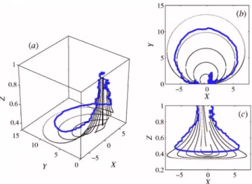
Figure2sketches the dynamics in the共X,Y ,Z兲 space. The line X = Y = 0 acts as a stable fixed line for the drift terms in Eqs.共4兲–共6兲. A typical trajectory spends a long time diffusing

around this line, until the noise realization becomes strong enough to escape from its neighborhood. When this happens with X⬎0, the quadratic terms in the drift drive the trajec-tory back to the stable line. On the contrary, if X⬍0 and hX2_{+ XZ − Y}2_{⬍0, the drift accelerates the trajectory towards}

larger negative values of X. Then the particles get closer to each other—i.e., Z decreases—until the quadratic terms in Eqs.共4兲 and 共5兲 become dominant. The trajectory then loops

back in the共X,Y兲 plane, approaching the stable line from its right.

During these loops, X becomes very large negative, and hence by Eq.共6兲, Z or equivalently the interparticle distance

R becomes substantially small. The loops are thus the basic mechanism for clustering. As we now show, their statistical signature is the presence of algebraic tails for the probability density function共PDF兲 of the dimensionless velocity differ-ences X and Y. Similarly to the case of smooth flows 关18兴

such power laws can be understood in terms of the cumula-tive probability P⬍共x兲=Pr共X⬍x兲 with xⰆ−1. The latter can be estimated as the product of 共i兲 the probability to start a sufficiently large loop that reaches values more negative than x and 共ii兲 the fraction of time spent by the trajectory at X⬍x. Therefore we assume that within a distance of order unity from the line X = Y = 0 the quadratic terms in the drift are negligible and X and Y are independent Ornstein-Uhlenbeck processes, while at larger distances only the qua-dratic terms contribute.

Within this simplified dynamics, a loop is initiated at a time s0for which X0= X共s0兲⬍−1 and Y0= Y共s0兲Ⰶ兩X0兩. If the

trajectory evolves on a loop in the共X,Y兲 plane, both 兩X共s兲兩 and Y共s兲 become very large. Let us denote by x* _{the largest}

negative value of X attained by the trajectory. Reaching val-ues smaller than xⰆ−1 is clearly equivalent to x*_{⬍x. Far}

from the stable line X = Y = 0, the noise can be neglected and the deterministic part of the dynamics can be integrated ex-plicitly. After some standard algebraic manipulations which are not detailed here, one obtains that x*_⬀关X

0+ Z0兴X0 h

Y₀−h. Hence, in order to reach values smaller than x, the loop should start with Y0⬍兩x兩−1/h. The probability to initiate such

a loop is thus given by the probability to exit the noise-dominated region with Y0⬍兩x兩−1/h. There, Y is approximately

an Ornstein-Uhlenbeck process, independent of X and Z and with a reflective boundary condition at Y = 0. Contribution共i兲 is thus⬀兩x兩−1/h. For the second contribution共ii兲, the fraction of time spent at X⬍x can be obtained from the explicit form of the solution when the noise is neglected; it is also found to be ⬀兩x兩−1/h_{. Put together, the two contributions give P}⬍_共x兲

⬀兩x兩−2/h_{when xⰆ−1. Hence the PDF of the longitudinal}

ve-locity difference X has a power-law tail p共x兲=dP⬍_{共x兲/dx⬀兩x兩}−␣ _{with exponent ␣= 1 + 2 / h. For}

smooth flows共h=1兲, one obtains␣= 3 as previously derived 关18兴. During the large loops, the trajectories equally reach

large positive values of X and of Y. Again the fraction of time spent at both X and Y larger than xⰇ1 can be estimated as x−1/h. Hence, the PDF of both X and Y have algebraic left and right tails.

As shown in Fig.3, the presence of power-law tails in the PDF is confirmed numerically, with perfect agreement be-tween the measured values of ␣ and the prediction

␣= 1 + 2 / h共see inset兲. Let us comment on the h dependence of␣. The probability to enter large loops, which correspond to events in which particles approach each other very closely 共i.e., the mechanism at the basis of particle clustering兲, de-creases significantly when h→0. Moreover, it is straightfor-ward to check from Eqs. 共4兲–共6兲 that during the loops

Z共s兲⬀Z0 h

when Z0Ⰶ1. Hence it gets less and less probable to

reach smaller values of Z as h decreases. Combined together, these two effects explain why particle clustering is weakened in rough velocity fields and why it is more efficient in smooth flows.

The change of variables 共7兲 can be equally applied in

FIG. 2.共Color online兲 Phase-space picture of the system 共4兲–共6兲

for h = 7 / 10. The thin smooth lines represent the drift. A random trajectory of the system withS共L兲=1 is shown in bold 共blue on-line兲; it performs a large loop from X⬍0 to X⬎0. 共a兲 The full 共X,Y ,Z兲 space, 共b兲 and 共c兲 projections in the Z=0 and Y =0 planes, respectively.

three dimensions, leading to a dynamics different from Eqs. 共4兲–共6兲. Therefore understanding to what extent the above

findings extend to the three-dimensional case remains an open question; work in this direction is under development.

To conclude, let us comment on the implications of this work to the study of heavy particles in real turbulent flows. There, particle clustering is simultaneously due to ejection from eddies and to a dissipative dynamics. The considered model flow isolates the latter effect. It is probable that power-law tails for velocity differences can be present in realistic settings as well. However, it is not clear if the results on clustering are affected by the presence of persistent struc-tures: particle ejection from eddies may form voids and thus very strong inhomogeneities in the particle distribution 关11,13兴. This could overtake dissipative-dynamics

mecha-nisms. Another effect neglected in this study is the presence of gravity, which can be important in many realistic situa-tions. Gravity provides a mechanism for the decorrelation of fluid velocity along particle paths. Therefore, including such an effect fits well in the time-uncorrelated model here dis-cussed and represents a natural continuation of the present work.

We acknowledge useful discussions with L. Biferale, G. Falkovich, K. Gawe¸dzki, A. Lanotte, S. Musacchio, and F. Toschi. This work has been partially supported by the EU network HPRN-CT-2002-00300 and by the French-Italian Galileo program “Transport and dispersion of impurities in turbulent flows.” The stay of R.H. in Nice was supported by the Zeiss-Stiftung and the DAAD.

关1兴 G. Falkovich, K. Gawedzki, and M. Vergassola, Rev. Mod. Phys. 73, 913共2001兲.

关2兴 C. Crowe, M. Sommerfeld, and Y. Tsuji, Multiphase Flows

with Particles and Droplets共CRC Press, New York, 1998兲.

关3兴 H. Pruppacher and J. Klett, Microphysics of Clouds and

Pre-cipitation共Kluwer Academic, Dordrecht, 1996兲.

关4兴 I. de Pater and J. Lissauer, Planetary Science 共Cambridge Uni-versity Press, Cambridge, England, 2001兲.

关5兴 W. Reade and L. Collins, Phys. Fluids 12, 2530 共2000兲. 关6兴 L. Zaichik, O. Simonin, and V. Alipchenkov, Phys. Fluids 15,

2995共2003兲.

关7兴 T. Elperin, N. Kleeorin, and I. Rogachevskii, Phys. Rev. Lett.

77, 5373共1996兲.

关8兴 E. Balkovsky, G. Falkovich, and A. Fouxon, Phys. Rev. Lett.

86, 2790共2001兲.

关9兴 J. Bec, J. Fluid Mech. 528, 255 共2005兲.

关10兴 H. Sigurgeirsson and A. Stuart, Phys. Fluids 14, 4352 共2002兲. 关11兴 G. Boffetta, F. De Lillo, and A. Gamba, Phys. Fluids 16, L20

共2004兲.

关12兴 P. Fevrier, O. Simonin, and K. Squires, J. Fluid Mech. 533, 1 共2005兲.

关13兴 L. Chen, S. Goto, and J. Vassilicos, J. Fluid Mech. 553, 143 共2006兲.

关14兴 U. Frisch, Turbulence: The Legacy of A. N. Kolmogorov 共Cam-bridge University Press, Cam共Cam-bridge, England, 1995兲. 关15兴 J. Eaton and J. Fessler, Int. J. Multiphase Flow 20, 169 共1994兲. 关16兴 G. Falkovich, A. Fouxon, and M. Stepanov, in Sedimentation

and Sediment Transport, edited by A. Gyr and W. Kinzelbach

共Kluwer Academic, Dordrecht, 2003兲, pp. 155–158. 关17兴 M. Maxey, J. Fluid Mech. 174, 441 共1987兲.

关18兴 J. Bec, M. Cencini, and R. Hillerbrand, Physica D 226, 11 共2007兲.

关19兴 A. Fouxon and P. Horvai 共unpublished兲. 关20兴 R. Kraichnan, Phys. Fluids 11, 945 共1968兲. 关21兴 L. Piterbarg, SIAM J. Appl. Math. 62, 777 共2002兲.

关22兴 B. Mehlig and M. Wilkinson, Phys. Rev. Lett. 92, 250602 共2004兲.

FIG. 3. PDF of X in log-log coordinates forS共L兲=1 and various values of h. In all cases, power-law tails are observed. Inset: expo-nent␣ of the algebraic tail as a function of the fluid velocity Hölder exponent h; the theoretical prediction is represented as a dotted line.

BEC, CENCINI, AND HILLERBRAND PHYSICAL REVIEW E 75, 025301共R兲 共2007兲