HAL Id: halshs-01026080
https://halshs.archives-ouvertes.fr/halshs-01026080
Submitted on 19 Jul 2014
HAL is a multi-disciplinary open access archive for the deposit and dissemination of sci-entific research documents, whether they are pub-lished or not. The documents may come from teaching and research institutions in France or
L’archive ouverte pluridisciplinaire HAL, est destinée au dépôt et à la diffusion de documents scientifiques de niveau recherche, publiés ou non, émanant des établissements d’enseignement et de recherche français ou étrangers, des laboratoires
What drives failure to maximize payoffs in the lab? A
test of the inequality aversion hypothesis
Nicolas Jacquemet, Adam Zylbersztejn
To cite this version:
Nicolas Jacquemet, Adam Zylbersztejn. What drives failure to maximize payoffs in the lab? A test of the inequality aversion hypothesis. Review of Economic Design, Springer Verlag, 2014, 18 (4), pp.243-264. �10.1007/s10058-014-0162-5�. �halshs-01026080�
What drives failure to maximize payoffs in the lab?
A test of the inequality aversion hypothesis
⇤Nicolas Jacquemet† Adam Zylbersztejn‡
June 2014
Abstract
Experiments based on the Beard and Beil (1994) two-player coordination game robustly show that coordination failures arise as a result of two puzzling behaviors: (i) subjects are not willing to rely on others’ self-interested maximization, and (ii) self-interested maximization is not ubiquitous. Such behavior is often considered to challenge the relevance of subgame perfectness as an equilibrium selection criterion, since weakly dominated strategies are actually used. We report on new experiments investigating whether inequality in payoffs between players, maintained in most lab implementations of this game, drives such behavior. Our data clearly show that the failure to maximize personal payoffs, as well as the fear that others might act this way, do not stem from inequality aversion. This result is robust to varying the saliency of decisions, repetition-based learning and cultural differences between France and Poland. Keywords: Coordination Failure, Subgame perfectness, Non-credible threats, Laboratory experiments, Social Preferences, Inequality Aversion.
JEL Classification: C72, D83.
∗This paper is a revised and extended version of CES Working Paper no
2011-36. We wish to thank an anonymous referee and an associate editor for their usefull comments. We are grateful to Juergen Bracht, Boˇgaçhan Çelen, Pierre-André Chiappori, Tore Ellingsen, Nick Feltovich, Guillaume Fréchette, Jacob Goeree, Frédéric Koessler, Stéphane Luchini, Rosemarie Nagel, Andreas Ortmann, Jean-Marc Tallon, Antoine Terracol, Marie-Claire Villeval and the participants to the Decision, Risk and Organization seminar at the Columbia Business School for their valuable comments; Maxim Frolov and Michal Krawczyk for their help in running the experiments; and Ivan Ouss and Anna Zylbersztejn for reasearch assistance. We acknowledge financial support from the University Paris 1 Panthéon-Sorbonne and the Paris School of Economics. Nicolas Jacquemet gratefully acknowledges the support of the Institut Universitaire de France. Adam Zylbersztejn is grateful to the Collège des Ecoles Doctorales de l’Université Paris 1 Panthéon-Sorbonne, the Alliance Program and the Columbia University Economics Department for their financial and scientific support.
†Université de Lorraine (BETA) and Paris School of Economics. 3 Place Carnot, 54035 Nancy.
Nicolas.Jacquemet@univ-lorraine.fr
‡Vienna University of Economics and Business – WU Wien, Department of Economics, Institute for Public
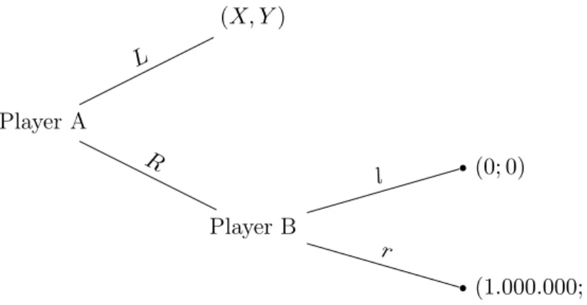
Figure 1: The Rosenthal (1981) game Player A Player B (1.000.000; 1) r (0; 0) l R (X, Y ) L
Note. 0 < X < 1.000.000. The value of Y is irrelevant from the strategic perspective. We assume 0 < Y < 1 so that the outcomes are Pareto-rankable.
1
Introduction
The game presented in Figure 1 illustrates the behavioral challenge posed by relying on the as-sumptions behind subgame perfectness. In this game, introduced by Rosenthal (1981), the first mover either decides alone on the outcome of the game (action R) or relies on the second mover (L). In the latter case, the second mover only has to decide whether to maximize both players’ payoffs (r) or not (l). Although the threat of non-maximization is non-credible and action l is ruled out by subgame perfectness, the first mover may still lose a substantial amount should the second mover fail to maximize payoffs. This makes the Pareto-dominated solution – in which the first mover plays L – a plausible case in real-life implementations. This puzzling behavioral outcome, originally introduced as a theoretical conjecture by Rosenthal, is robustly highlighted by all lab experiments using both sequential-move and simultaneous-move versions of the game.1 Suboptimal outcomes arise due to two different driving forces: first, as expected by Rosenthal, subjects who play as first movers are very frequently reluctant to rely on second movers; second, surprisingly enough, an important share of second movers do indeed turn out to be unreliable and fail to maximize both players’ payoffs.
Such evidence has long been seen as a pathological example of people’s inability to use subgame perfectness. This interpretation however relies on the assumption of standard preferences that only include personal payoffs – so that the common knowledge of the payoff scheme provides complete information about all players’ preferences. The aim of this paper is to investigate another possible
1
The experimental literature on this game has been initiated by the seminal study by Beard and Beil (1994) and is reviewed in details below. An advantage of the simultaneous-move implementation used in this paper is that both players make decisions independently, so that their behavior is always observable to the experimenter.
explanation for these puzzling behaviors, namely inequality aversion (Fehr and Schmidt, 1999) – which may rationalize suboptimal outcomes in all the payoff structures implemented to date in lab experiments.2 Our investigation is based on two research questions: do unequal payoffs generated by the dominant outcome (i) make second movers unwilling to maximize both players’ payoffs, and (ii) make first movers reluctant to rely on second movers that are actually reliable? We implement six variations of the payoff structure of the game, all sharing the main strategic dimensions of the original game. The Baseline treatments are compared to Egalitarian treatments which restore equality between players’ payoffs in the Pareto-dominant outcome. We also assess the robustness of our results to enhanced saliency of the decisions in the game, and provide evidence on the cross-cultural robustness by collecting data in France and in Poland.
Our findings are threefold. First, our data unambiguously reject the inequality aversion hy-pothesis, since neither the behavior of the first movers nor the behavior of the second movers changes due to equalized payoffs. Second, we observe that payoff maximization among second movers is almost universal only once all the Nash equilibria in the game involve the same in-equality of payoffs. This suggests that player Bs in other treatments – where player As’ relative standing in the non-cooperative equilibrium is more favorable than in the cooperative one – might act inefficiently so as to penalize their partners for enjoying an undeserved procedural advantage. This points to a totally different kind of other-regarding preferences, related to procedural justice.3 Our third finding is that first movers do not take into account this transition in second movers’ behavior, as if they did not expect social preferences to have any effect on their partners’ actions. We conclude the paper with a discussion of the avenues that remain open to explain such a robust inefficiency observed in the lab.
2
Two puzzling behaviors in existing laboratory experiments
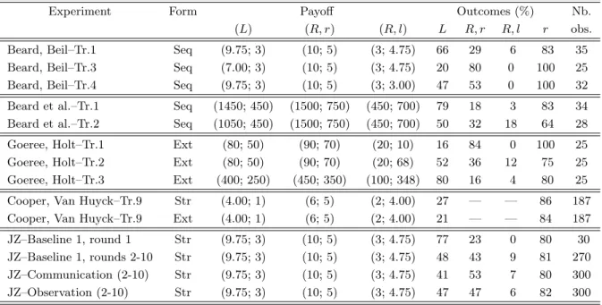
Table 1 provides an overview of previous experimental implementations of the game studied in this paper. There are only three different outcomes in the game, detailed in the left-hand side of the
2
The extent to which this preference explains the divergence between human decisions and standard game-theoretical predictions is the subject of a lively debate in experimental economics. For instance, lab experiments by Charness and Grosskopf (2001), Kritikos and Bolle (2001), Charness and Rabin (2002) and Engelmann and Strobel (2004) provide evidence against the inequality aversion hypothesis, while subsequent experiments by Chmura, Kube, Pitz, and Puppe (2005), Fehr, Naef, and Schmidt (2006), Bolton and Ockenfels (2006), Blanco, Engelmann, and Normann (2011), as well as a neuroeconomic study by Tricomi, Rangel, Camerer, and O’Doherty (2010), report evidence in its favor.
3
Krawczyk (2011, p.112) defines procedural justice as “transparent and impartial rules ensuring that each of the agents involved in an interaction enjoys an equal opportunity to obtain a satisfactory outcome.” In this approach to other-regarding preferences, the individual utility depends not only on the type of achieved outcomes, but also on the way in which they were generated. As discussed in the concluding section, there exists previous experimental evidence that people exhibit a taste for procedural justice and are even willing to sacrifice their own wealth for punishing those who enjoy an undeserved procedural advantage.
Table 1: Summary of experimental evidence on Rosenthal’s game
Experiment Form Payoff Outcomes (%) Nb.
(L) (R, r) (R, l) L R, r R, l r obs. Beard, Beil–Tr.1 Seq (9.75; 3) (10; 5) (3; 4.75) 66 29 6 83 35 Beard, Beil–Tr.3 Seq (7.00; 3) (10; 5) (3; 4.75) 20 80 0 100 25 Beard, Beil–Tr.4 Seq (9.75; 3) (10; 5) (3; 3.00) 47 53 0 100 32 Beard et al.–Tr.1 Seq (1450; 450) (1500; 750) (450; 700) 79 18 3 83 34 Beard et al.–Tr.2 Seq (1050; 450) (1500; 750) (450; 700) 50 32 18 64 28 Goeree, Holt–Tr.1 Ext (80; 50) (90; 70) (20; 10) 16 84 0 100 25 Goeree, Holt–Tr.2 Ext (80; 50) (90; 70) (20; 68) 52 36 12 75 25 Goeree, Holt–Tr.3 Ext (400; 250) (450; 350) (100; 348) 80 16 4 80 25 Cooper, Van Huyck–Tr.9 Str (4.00; 1) (6; 5) (2; 4.00) 27 — — 86 187 Cooper, Van Huyck–Tr.9 Ext (4.00; 1) (6; 5) (2; 4.00) 21 — — 84 187 JZ–Baseline 1, round 1 Str (9.75; 3) (10; 5) (3; 4.75) 77 23 0 80 30 JZ–Baseline 1, rounds 2-10 Str (9.75; 3) (10; 5) (3; 4.75) 48 43 9 81 270 JZ–Communication (2-10) Str (9.75; 3) (10; 5) (3; 4.75) 41 53 7 80 300 JZ–Observation (2-10) Str (9.75; 3) (10; 5) (3; 4.75) 47 47 6 82 300
Note.Several representations of the game have been applied so far, as stated in column 1: simultaneous-move strategic-form game (Str), simultaneous-move extensive-form game (Ext), sequential-move game (Seq). Player Bs’ actions r in the first three studies are only reported conditional on player As’ action R. The monetary payoffs displayed in columns 2-4 are in USD in Beard & Beil (1994) and Cooper & Van Huyck (2003), in US cents in Goeree & Holt (2001), in yens in Beard et al. (2001) and in euros in Jacquemet & Zylbersztejn (2013, JZ) treatments.
table: either the first mover (henceforth player A) chooses to decide alone by picking L, or he relies on the second mover’s (henceforth player B’s) decision by choosing R. In this case, both players’ payoffs are higher if r is chosen rather than l. The right-hand side of the table summarizes each outcome as a percentage of all observed decisions, as well as the frequency of action r conditional on reliance from player A.
The main focus of the original study by Beard and Beil (1994) is to test Rosenthal’s conjecture that subjects may be unwilling to rely on the other players’ ability to maximize payoffs – hence challenging subgame perfectness.4 Their experimental evidence supports the Rosenthal conjecture:
although the share of payoff-maximizing subjects is high in the sub-population of player Bs who are relied upon (from 83% in their treatment 1 to 100% in treatments 3 and 4, for instance), most player As decide not to rely on their partners. The comparison across treatments shows that behavior highly depends on the size of stakes: the lower the value of the secure option, the higher the reliance rate from player As; the higher the cost of being unreliable, the higher the reliability
4
Subgame perfectness refines the Nash equilibrium through the iterative elimination of weakly dominated strat-egy – which are non-credible threats in the sequential game. The failure to maximize payoff in the game we study precisely amounts to using weakly-dominated strategies. See Jacquemet and Zylbersztejn (2013) for a more detailed analysis of the theoretical properties of the game.
rate from player Bs. Beard, Beil, and Mataga (2001) replicate some of these treatments using Japanese subjects. While the results of their treatment 1 are in line with previous US evidence, behavior in treatment 2 is in a sense more striking. Because of the increase in the monetary incentives to reach (R, r) as compared with the secure outcome (L), a much higher share of player As rely on their partner – from 21% in treatment 1 to 50% in treatment 2. However, although the payoffs for player B remain unchanged between the two treatments, the share of payoff-maximizing decisions (conditional on having been relied upon in the first place) falls from 83% to 64%.
Importantly, both of these studies elicit decisions from player Bs conditional on the prior reliance of player As. Hence, this evidence does not suffice to infer the actual behavior in the entire population of player Bs, since the decisions of player Bs paired with unreliant player As cannot be observed. In contrast, Goeree and Holt (2001) and Cooper and Van Huyck (2003) use a simultaneous-move game of either normal or extensive form, and confirm the robustness of previous evidence. First, even when player Bs are actually reliable (such as in the Goeree and Holt treatment 1), a large share of player As are reluctant to rely on them. Second, in a large variety of treatments (treatments 2 and 3 in Goeree and Holt and both treatments of Cooper and Van Huyck) player Bs actually are often unreliable – decision r occurs from 15% to 25% of the time. Jacquemet and Zylbersztejn (2013) study the role of the amount of information about interaction partners acquired through three different channels: repetition-based learning, cheap talk communication from player B to player A and observation of player B’s past actions by player A . To that end, the experiment implements the normal form of the game and thus elicit decisions in the whole population of player As and player Bs. In the initial round of their baseline treatment (last two rows of Table 1), 23% of player As prefer the secure choice and 100% of player Bs that are relied upon actually turn out to be reliable. This proportion is, however, much lower (80%) in the whole population of player Bs they could be matched with. Evidence from nine subsequent rounds of the same game (where repetition takes place under a perfect-stranger design with fixed roles and round-robin matching) suggests that learning is of very little help in disciplining that behavior – the overall frequency of reliable decisions from player Bs amounts to 81%. More generally, this behavior on the part of player Bs is insensitive to any of the experimental treatments, as shown in the last two rows of the Table. This means that neither repetition-based learning, nor forward-looking information through messages, nor even backward-forward-looking information from observation of past decisions suffices to discipline player Bs’ choices of weakly-dominated actions in this payoff configuration.
3
Empirical strategy
From existing experimental evidence, two puzzling behaviors arise: a large share of player As appear reluctant to rely on actually reliable player Bs; but at the same time the weakly-dominated strategy is often chosen by player Bs. The purpose of this paper is to test whether such behavior
Table 2: Generic game
player B
player A l r
L (a;b) (a;b)
R (a-c;b-e) (a+d;b+f)
is related to the payoff structure of the game.5 To illustrate the point, the general structure of
the game is presented in Table 2 – of which all the lab implementations presented in Table 1 above are particular cases. The crucial properties of the game hold if the parameters a, . . . , f take non-negative values and all payoffs are positive. Player B (weakly) maximizes both players’ payoffs by selecting r, while player A prefers L to the outcome (R, l) that is attained when relying on an unreliable player B . As a result, the game has two Nash equilibria, (L, l) and (R, r). The first is imperfect (since it entails player B’s weakly dominant strategy l), while the second is (trembling-hand) perfect and Pareto-superior.
But in most experimental implementations of this game, the payoffs from the perfect Nash equilibrium are much higher for player A than for player B , i.e., a ≥ b, a + d ≥ b + f , b − e ≥ a − c. Although this does not make B’s unreliable decision l a rational answer to A’s reliance, non-standard preferences involving inequality aversion might explain why player Bs forgo efficiency at a personal monetary cost (Fehr and Schmidt, 1999). Moreover, if player As believe that this sort of preference exists among player Bs, they may prefer to choose the secure option instead of relying on their partner. In order to test this hypothesis, our empirical approach consists in complementing the original payoff structure with variations that maintain the strategic properties of the game, while equalizing the payoffs both players earn in the case of payoff-maximizing coordination, i.e.,
5
This hypothesis has been already raised in the literature – see for instance (Goeree and Holt, 2001, p.1416) – but to the best of our knowledge it has never been examined empirically. One exception is treatment 6 in Beard and Beil (1994), discussed in Section 3.1. Surprisingly, this treatment is not commented on in the original paper, neither it is discussed as a means to assess the sensitivity of behavior to more equalized payoffs. In any case, as stressed above, the original design of Beard and Beil (1994) is inappropriate for studying player Bs’ behavior, since their decisions are elicited only conditional on player A’s choice.
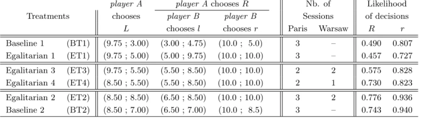
Table 3: Overview of experimental treatments
player A player Achooses R Nb. of Likelihood Treatments chooses player B player B Sessions of decisions
L chooses l chooses r Paris Warsaw R r Baseline 1 (BT1) (9.75 ; 3.00) (3.00 ; 4.75) (10.0 ; 5.0) 3 – 0.490 0.807 Egalitarian 1 (ET1) (9.75 ; 5.00) (5.00 ; 9.75) (10.0 ; 10.0) 3 – 0.457 0.727 Egalitarian 3 (ET3) (9.75 ; 5.50) (5.50 ; 8.50) (10.0 ; 10.0) 2 2 0.575 0.828 Egalitarian 4 (ET4) (8.50 ; 5.50) (5.50 ; 8.50) (10.0 ; 10.0) 2 1 0.730 0.823 Egalitarian 2 (ET2) (8.50 ; 8.50) (6.50 ; 8.50) (10.0 ; 10.0) 3 2 0.776 0.936 Baseline 2 (BT2) (8.50 ; 7.00) (6.50 ; 7.00) (10.0 ; 8.5) 3 – 0.743 0.940
Note. For each treatment, the first three columns provide the payoffs of each player, in euros. The next two columns give the number of 20 subjects-sessions run in each location. The last two columns summarize the average behavior observed in each treatment over all subjects and repetitions.
such that (a + d) = (b + f ).6
3.1 Overview of the experimental design
Table 3 summarizes our experimental design, which uses 6 payoff configurations (described in subsequent rows) and 2 different locations (described in the middle columns). They seek to address three empirical questions related to inequality aversion. First, we address the question of whether the equality-based preferences affect equilibrium selection by restoring payoff equality between players. Second, we investigate the interplay between saliency and equality concerns by increasing the opportunity cost of dominated actions. Third, following a related cross-cultural study by Beard, Beil, and Mataga (2001), we seek to identify potential cultural differences in
6
The treatment effects we seek to identify are best illustrated in the framework of the Fehr and Schmidt (1999) model of inequality-aversion. Both subjects i, j 2 {A, B} are assumed to choose their actions in the game presented in Table 2 according to the extended utility function defined on outcome O generating payoffs (Oi; Oj):
Ui(O|αi, βi) = Oi− αi⇤ (Oj− Oi) ⇤ 1Oi<Oj − βi⇤ (Oi− Oj) ⇤ 1Oi>Oj (1) Parameters 0 βi αi measure the sensitivity of player i to inequality (1Oi<Oj = 1 − 1Oi>Oj = 1 if j earns
more than i, 0 otherwise). The payoff structures of our Baseline Treatments (BT1 and BT2 in Table 3) are such that 9(αB, βB) : UB((R, l)BT|αB, βB) > UB((R, r)BT|αB, βB), so that a player B whose utility is defined
by (1) may prefer outcome (R, l) over (R, r). By the same token, Egalitarian Treatments (ET1-4 in Table 3) are built in such a way that 8(αB, βB) : UB((R, l)ET|αB, βB) < UB((R, r)ET|αB, βB), so that for the same preference
parameters, player B now prefers (R, r) over (R, l). As for player As, define θTas the perceived likelihood that player
Bs’ realization of (αB, βB) makes him prefer (R, l) over (R, r) in Treatment T . If player A is an expected utility
maximizer, then EUA(RT|αA, βA, θT) = θTUA((R, l)T|αA, βA) + (1 − θT)UA((R, r)T|αA, βA). As a result, if the fear
that player Bs are inequality-averse is high enough, player A may prefer the secure choice in the Baseline Treatment, since 9(αA, βA, θBT) : UA(LBT|αA, βA) ≥ EUA(RBT|αA, βA, θBT). By contrast, the Egalitarian Treatment is
preferences by comparing the behavior of French and Polish subjects. The differences from one treatment to the other are described in turn below.
Inequality aversion under weak saliency. Our starting point is Baseline Treatment 1 – which corresponds to the Beard and Beil (1994) treatment 1 and the Jacquemet and Zylbersztejn (2013) replication – which gives rise to the two puzzling behaviors we are interested in. To this treatment, we associate an egalitarian version, Egalitarian Treatment 1 that equalizes payoffs in the Pareto efficient outcome – also used as treatment 6 in Beard and Beil (1994). As shown in the last two columns of the table, presenting the observed proportions of reliant decisions (R) from player As and reliable decisions (r) from player Bs, equalizing payoffs in the Pareto-efficient outcome has virtually no effect on players’ average behavior.
Behavioral effect of enhanced saliency. An important shortcoming of the first pair of treat-ments is that saliency may be violated, as reliance and reliability only induce a 0.25 euro variation in subjects’ payoffs. Two additional treatments seek to assess the robustness of the results to this feature. In Egalitarian Treatment 3, built on ET1, we improve the saliency of reliable decisions for player B : the opportunity cost of playing r (instead of the weakly dominated decision l) against Ris now 1.5 euros.7 Similarly, in Egalitarian Treatment 4 based on ET3, we improve the saliency of being reliant for player A – the payoff difference between the two Nash equilibria amounts to 1.5 euros instead of 0.25 euros. In both of these treatments, we maintain equality in payoffs between players in the Pareto-efficient outcome. The comparison between ET3 and ET1 thus allows to identify the effect of saliency on player B’s reliability in an equalized payoffs environment ; while the comparison between ET3 and ET4 similarly highlights the effect of saliency on player A’s reliance. We derive mixed results from these two additional treatments: the behavior of player Bs is unaffected by both changes, while the share of reliant decisions from player As is significantly higher in ET4 than in ET1 and ET3.
Inequality aversion under enhanced saliency. In all treatments described up till now, a strong payoff inequality between players remains if player A chooses L. As a result, it could be that A’s choice of being reliant is itself driven by the willingness to move away from outcomes with too much inequality in payoffs. In Egalitarian Treatment 2, built on ET4, we restore equality in the dominated equilibrium by raising player B’s payoff.8 The comparison between ET2 and ET4 thus seeks to identify the effect of player As’ inequality aversion on the outcomes. Surprisingly enough, the main lesson drawn from this comparison is that ET2 strongly disciplines the behavior
7
In the course of trials leading to the current experimental treatments, we also slightly raised all payoffs from 5.0 in ET1 to 5.5 in ET3, to verify whether decimals have any effect on players’ behavior.
8
By the same token as above, we slightly raise the payoff earned by player A in the event of unsuccessful attempts to rely on B, from 5.5 to 6.5.
of player Bs – the weakly dominated action is now almost never chosen. The behavior of player As, by contrast, is unaffected by this change. To assess whether such a high rate of secure choices – despite widespread reliability in the population of player Bs – is reinforced by payoff inequality, we complete our design with Baseline Treatment 2, built on ET2, in which the Pareto-dominant outcome gives rise to payoff inequality in favor of player A.9 Again, we fail to find any effect of this dimension of the game, as both players behave in the same manner as in ET2.
Cross-cultural comparison. All our main treatments of interest were run in Paris (France). The last concern our design addresses is the possibility that the treatment effects are driven by culture-specific motives. To assess the robustness of our results to this dimension, we run additional sessions in Warsaw (Poland).10 We chose the three treatments in which observed behavior is in our view the most striking, i.e. ET2, ET3 and ET4. The number of sessions in each location is provided in Table 3.
3.2 Experimental procedures
Each payoff variation described above defines a treatment, and all treatments are implemented separately using a between-subject design. The design is kept the same for all treatments, based on the procedures of Jacquemet and Zylbersztejn (2013).
We introduce two important changes to Beard and Beil’s original design. First, we study the effect of learning by repeating the one-shot game 10 times.11 Each occurrence is one-shot in the sense that: roles are fixed; pairs are re-matched in each round using a perfect-stranger, round-robin procedure; we avoid the end-game effect by providing no information about the exact number of repetitions; and take-home earnings are derived from one round, randomly drawn out of the ten at the end of each experimental session. Second, we elicit both players’ decisions in each occurrence of the game. In that respect, we break the original sequentiality of the game and ask each player
9
In designing this treatment, we seek to introduce payoff inequality between players, while holding constant the saliency of being reliable for player B . We thus choose to reduce player B’s payoff in (R, l) to 7.00, instead of 8.50 in ET2, and accordingly adjust the payoff stemming from decision L.
10
As an Eastern European country, Poland seems to sufficiently differ in political and social history from France to serve the purpose of a robustness check of our results to a different cultural background. In particular, experimental evidence suggests that social preferences (like trust and reciprocity) may vary across European countries (Willinger, Keser, Lohmann, and Usunier, 2003). This robustness treatment complements the contribution of Beard, Beil, and Mataga (2001), who use the data from USA and Japan to show that inefficient behavior in Rosenthal’s game persists across cultures. It should be stressed, however, that this treatment does not aim to provide a thorough cross-cultural comparison, but rather to rule out the possibility that our main treatment effects of interest are specific to the location of our experiments.
11
Although Rosenthal made his conjecture for a one-shot game, Beard and Beil note in their paper (pp. 261-262) that it seems equally valid for repeated play. The authors furthermore state that learning through experience may affect people’s behavior independently of payoff-related factors.
for unconditional choices in each round. Players are only informed about their own payoffs at the end of each round.
A typical session proceeds as follows. Upon arrival, subjects sign an individual consent form. They then enter the lab, where they are randomly assigned to their computers and asked to fill in a small personal questionnaire containing basic questions about their age, gender, education, etc. The written instructions are then read aloud. Players are informed that they will play some (unrevealed) number of rounds of the same game, each round with a different partner, and that their own role will not change during the experiment. Before starting, subjects are asked to fill in a quiz assessing their understanding of the game they are about to play. Once the quiz and all remaining questions have been answered, the experiment begins. Prior to the first round, players are randomly assigned to their roles – either A or B. They are then anonymously and randomly matched to a partner and asked for their choice: R or L for player As, r or l for player Bs. At the end of each round, each player is informed only about their own payoff. When all pairs have completed a round of the game, the subjects are informed whether or not a new round is starting. In the event of a new round, pairs are re-matched according to a perfect-stranger matching procedure (any pair meets only once in the session). At the end of the experiment, one round is randomly drawn and each player receives the amount corresponding to their gains in that round plus a show-up fee.
All in all, we ran a total of 21 experimental sessions: 16 in the Laboratoire d’Economie Ex-perimentale de Paris (LEEP) at University Paris 1 Panthéon-Sorbonne, between June 2009 and January 2012, and 5 in the Experimental Economics Laboratory at Warsaw University in February 2012.12 In both laboratories, subjects were recruited via an online registration interface adapted
using Orsee (Greiner, 2004) and the experiment was computerized using software developed un-der Regate (Zeiliger, 2000). Each session lasted about 45 minutes, with an average payoff of 14 euros in Paris and 28 PLN (about 7 euros) in Warsaw.13 No subject participated in more than one experimental session. Out of 420 participants, 206 were men and 214 were women. A vast majority of the population (332 subjects) were students in various disciplines, and 193 of them were likely to have some knowledge of game theory due to their field of study.14 297 subjects had taken part in economic experiments before. The average age of the participants was 24.
12
Data from the sixth session run in Warsaw, implementing ET4, have been lost as a result of a software crash.
13
For French subjects, all the payoffs in experimental instructions were expressed in euros. For Polish subjects, we use the same payoff scheme, but expressed in Experimental Current Units (ECU). For the purposes of payment, ECU were converted to Polish Zloty (PLN) at the rate 1 ECU=2 PLN. The participation fee was 5 euros in Paris and 10 PLN (around 2.5 euros according to the current exchange rate in 2012) in Warsaw. Since a vast majority of our subjects are students, and petty student jobs usually pay about 8 euros per hour in Paris and 15 PLN per hour in Warsaw, we strongly believe that the participants’ monetary incentives are comparable between countries.
14
Disciplines such as economics, engineering, management, political science, psychology, applied mathematics for the social sciences, mathematics, computer science, and sociology.
4
Results
In what follows, statistical inference is based on between-treatment tests for the significance of differences in the proportions of each outcome of interest. We use two kinds of statistical tests. In round 1, where all observations are independent, we use two-sided Fisher’s exact tests. In rounds 2-10, individual observations may be correlated within each session due to the re-matching of subjects from one round to the other. We take into account this data structure by using the following parametric procedure. First, we run an OLS regression of treatment dummies on a dummy dependent variable representing the outcome of interest. In this setup, coefficients correspond to the proportions of outcomes of interest in a given treatment, so that two-sided t-tests and F -t-tests on coefficients allow us to test linear hypotheses about the equality of proportions between treatments. To take into account the within-session correlation, we cluster data at the session level, and use leave-one-out jackknife standard errors to deal with the issue of potential small-sample bias. This method is applied to data from rounds 1-10 and 2-10.15
To ease the description of observed behavior, we use the following nomenclature. A cooperative decision means R (r) for player As (Bs). A cooperative outcome accordingly corresponds to the Pareto-Nash equilibrium (R, r), while a coordinated outcome describes a situation where either of the existing Nash equilibria – (L, l) or (R, r) – is attained. Last, we also consider two types of miscoordination (corresponding to different non-equilibrium outcomes): (L, r) and (R, l).
4.1 Replication of Beard and Beil’s treatments
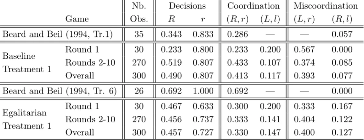
Our first comparison of interest is BT1 against ET1, two treatments previously studied by Beard and Beil (1994). In Table 4, we summarize the main outcomes from both their and our implemen-tations of these two treatments. The data collected by Beard and Beil in the context of a one-shot sequential-move game seem to favor the inequality aversion hypothesis. The rate of reliance by player As doubles, from 34.3% (12 cases out of 35) in the Baseline Treatment 1 to 69.3% (18/26) in the Egalitarian Treatment 1 (p=0.010), and the rate of conditional reliability from player Bs increases from 83.3% (10/12) to 100% (18/18) (p=0.152). Therefore, player As do indeed act more cooperatively in an environment where bilateral cooperation gives equal profits to both partners, and player Bs actually seem to prefer an equal division of the gains for cooperation, although the magnitude of this preference is marginal.
Our replication of both treatments in a repeated simultaneous-move game yields results that are more mixed and – most importantly – non-persistent. For inexperienced player As (actions observed in round 1), the likelihood of action R also doubles, as in Beard and Beil’s study, in-creasing from 23.3% in BT1 to 46.7% in ET1 (p=0.103), but player Bs are at the same time marginally less reliable – the frequency of cooperative choices falls from 80% to 63.3% (p=0.252).
15
Table 4: Observed behavior in Treatments 1
Nb. Decisions Coordination Miscoordination Game Obs. R r (R, r) (L, l) (L, r) (R, l) Beard and Beil (1994, Tr.1) 35 0.343 0.833 0.286 — — 0.057 Baseline
Treatment 1
Round 1 30 0.233 0.800 0.233 0.200 0.567 0.000 Rounds 2-10 270 0.519 0.807 0.433 0.107 0.374 0.085 Overall 300 0.490 0.807 0.413 0.117 0.393 0.077 Beard and Beil (1994, Tr. 6) 26 0.692 1.000 0.692 — — 0.000 Egalitarian
Treatment 1
Round 1 30 0.467 0.633 0.300 0.200 0.333 0.167 Rounds 2-10 270 0.456 0.737 0.333 0.141 0.404 0.122 Overall 300 0.457 0.727 0.330 0.147 0.400 0.127
Note. For each treatment (in rows), the first column gives the total number of observations – the number of subjects is equal to N in Beard and Beil’s experiment, and N/10 in ours. The two subsequent columns present the individual decisions observed in each treatment (the rate of reliability is conditional on reliance from player A in Beard and Beil’s data and unconditional in ours). The last four columns present the empirical frequencies of the four possible outcomes (two of which – (L, l) and (L, r) – are not observable in Beard and Beil’s data).
Importantly, these differences completely disappear among experienced players (actions observed in rounds 2-10), where subjects’ behavior is virtually identical under both conditions: the frequency of decisions R varies between 51.9% in BT1 and 45.6% in ET1 (p=0.574), while the frequencies of decisions r by player Bs are 80.7% and 73.7% (p=0.602).16
4.2 Inequality aversion under improved saliency
Table 5 summarizes the outcomes from our four companion treatments, along with a reminder of the main results from BT1 and ET1. For the three egalitarian treatments (ET2, ET3 and ET4), we split the results according to the location of the experiment. This allows us to assess the level of cultural specificity in the behavior observed in this game.
In the light of the data from these three treatments, it is difficult to argue that there is any systematic difference between the patterns of behavior in each country. Player As’ behavior is only subject to minor discrepancies and seems quite similar in France and Poland. For treatments ET2 and ET4, players Bs’ behavior in both countries is practically identical. The sole visible difference concerns player Bs’ behavior in treatment ET3, where Polish subjects are slightly more likely to select action r than French subjects. However, statistical tests are unable to reject the
16
In line with individual behavior, outcomes do not react much to treatment. Overall, only 53% of outcomes in BT1, and 47.7% in ET1 (p=0.249), are coordinated. Cooperative outcomes account for 41.3% and 33% (p=0.497), respectively. Miscoordination (L, r) is extremely widespread, attaining 39.3% and 39.7% (p=0.955) of global out-comes. The most costly miscoordination (R, l) is also pronounced, reaching 7.7% and 12.7% (p=0.220) in BT1 and ET1, respectively.
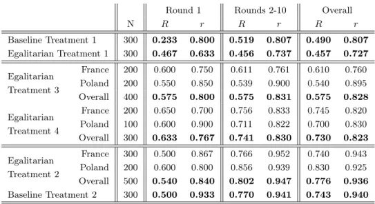
Table 5: Observed decisions
Round 1 Rounds 2-10 Overall
N R r R r R r Baseline Treatment 1 300 0.233 0.800 0.519 0.807 0.490 0.807 Egalitarian Treatment 1 300 0.467 0.633 0.456 0.737 0.457 0.727 Egalitarian Treatment 3 France 200 0.600 0.750 0.611 0.761 0.610 0.760 Poland 200 0.550 0.850 0.539 0.900 0.540 0.895 Overall 400 0.575 0.800 0.575 0.831 0.575 0.828 Egalitarian Treatment 4 France 200 0.650 0.700 0.756 0.833 0.745 0.820 Poland 100 0.600 0.900 0.711 0.822 0.700 0.830 Overall 300 0.633 0.767 0.741 0.830 0.730 0.823 Egalitarian Treatment 2 France 300 0.500 0.867 0.766 0.952 0.740 0.943 Poland 200 0.600 0.800 0.856 0.939 0.830 0.925 Overall 500 0.540 0.840 0.802 0.947 0.776 0.936 Baseline Treatment 2 300 0.500 0.933 0.770 0.941 0.743 0.940
Note.For each treatment (in rows), the second column gives the number of observations – the number of individual subjects is N/10. For the first round of play, Rounds 2-10 and overall averages, the three sub-columns provide the average frequency of reliance from player A (decision R) and reliability from player B (decision r).
null of equal means in the two countries.17 We therefore do not consider the cultural background
as an influential factor in our experimental data, and accordingly pool both locations in the data analysis below.
In ET3 and ET4, we improve the saliency of the action leading to the Pareto-efficient outcome for each player in turn. As compared to ET1, ET3 increases player Bs’ conditional surplus from playing r, while ET4 also increases player As’ conditional surplus from playing R. Comparing these three experimental conditions, we observe very little variation in player Bs’ actions: although reliable decisions are observed slightly more often when incentives become more salient – for instance, in 63% of round 1 decisions in ET1 compared with 80% in ET3 and 77% in ET4 – we cannot identify any statistically significant difference.18
Setting ET1 as a benchmark, conditions ET3 and ET4 also allow us to investigate two impor-tant issues concerning player As’ decision-making. First, do player As react to partners’ enhanced incentives to act reliably in ET3 – notwithstanding player Bs’ actual neutrality? Second, do player
17
The Kolmogorov-Smirnov test using all session averages does not detect differences between the two countries either in the population of player As (p = 0.980) or in the population of player Bs (p=0.317). We can only test the nullity of the difference for each treatment separately in the first round, when individual decisions are not correlated. The p-values are p=0.569 in ET2, and p=1 in ET3 and ET4 for player As, and p=0.697, p=0.695, p=0.372 for player Bs. The results from parametric regressions (see Section 5) confirm this conclusion.
18
The p-values from mean differences between treatments ET1 and ET3/ET4 are p=0.175/p=0.399 in round 1, p=0.491/p =0.461 in rounds 2-10, and p=0.446/p=0.418 in rounds 1-10. The null hypothesis that behavior is the same in all three treatments cannot be rejected in round 1 (p=0.290), in rounds 2-10 (p=0.753), or in rounds 1-10 (p=0.710).
As react to the enhancement of their own incentives to rely on their partners in ET4? Based on our data, the answer to the first question is clearly negative: the improvement of the saliency of player Bs’ decisions between ET1 and ET3 only results in a marginal and statistically insignificant drop in the frequency of player As’ secure choices.19 The answer to the second question, on the
contrary, appears to be positive. Although ET4 brings no significant improvement in term of player As’ reliance in the initial round, the increase in the rate of reliability becomes highly signif-icant in subsequent rounds.20 Note that player Bs’ behavior is similar in all three treatments (in particular in ET3 and ET4). The observed change in player As’ behavior is thus mainly driven by the enhanced saliency of their personal payoffs ; rather than updated beliefs about the reliability of the partner.
ET2 is designed to detect another potential motivation underlying reliance: as compared with ET4, payoffs generated by a secure choice are equalized, so that we should observe a fall in reliance if player As use decision R to move away from outcomes with highly unequal payoffs. We clearly reject this hypothesis both in the first round (p=0.487) and in subsequent repetitions (p=0.539). On the other hand, we find a strong effect on player Bs’ behavior after the first round (where the rate of decisions r equals 84%). In this version of Egalitarian Treatment, subjects in the role of player B attain the highest proportion of decisions r, with almost 95% of actions r in rounds 2-10.21 We complete our design by considering a variation of ET2, in which the payoffs associated with the Pareto-dominant outcome are unequal between players. The comparison between BT2 and ET2 thus complements BT1-ET1 in a context in which payoff differences are salient and the payoff differences are equalized between players in both Nash equilibria of the game. Once again, we find no important inter-treatment differences in either player As’ or player Bs’ actions.22
Altogether, BT2 and ET2 provide the unique experimental environment where player Bs’ reliable behavior is almost universal. Importantly, these games hold the payoff inequality constant across the Nash equilibria. This feature neutralizes the procedural advantage that player A holds over player B in the remaining games: ending the game with the safe action L rather than setting out to achieve (R, r) no longer generates disproportionately higher losses to player B than to player A. According to this interpretation, player Bs’ inefficient behavior in our experiment is related to
19
p=0.469 in round 1, p=0.249 in rounds 2-10, p =0.193 in rounds 1-10.
20
In round 1: p=0.469 against ET1, p=0.809 against ET3; in rounds 2-10: p=0.013 against ET1, p=0.004 against ET3; for rounds 1-10: p=0.008 against ET1, p=0.007 against ET4. Although we cannot reject the null hypothesis that subjects’ behavior in round 1 is the same in all three treatments (p=0.462), we can do so for rounds 2-10 (p=0.006) and rounds 1-10 (p=0.007).
21
Comparing ET2 against ET3: p=0.782 in round 1, p=0.081 in rounds 2-10, and p=0.104 in rounds 1-10. Comparing ET2 against ET4: p=0.555 in round 1, p=0.006 in rounds 2-10, and p=0.001 in rounds 1-10. Although we cannot reject the null hypothesis that subjects’ behavior in round 1 is the same in all three treatments (p=0.701), we can do so for rounds 2-10 (p=0.012) and rounds 1-10 (p=0.003).
22
For player As, we find p=0.819 in round 1 and p=0.745 in rounds 2-10;, p=0.741 in rounds 1-10. For player Bs, p=0.306 in round 1 and p=0.858 in rounds 2-10; p=0.902 in rounds 1-10.
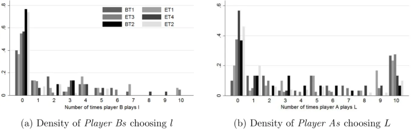
Figure 2: Empirical distribution of players according to their actions
(a) Density of Player Bs choosing l (b) Density of Player As choosing L
Note. The figures report the distributions of the number of player Bs and player As according to the number of times decision l/L is chosen over the 10 repetitions of the game.
procedural fairness and arises as a costly punishment of those who enjoy an undeserved strategic advantage. We further discuss this explanation in the concluding section.
To get further insight into individual behavior, we reorganize the data at the individual level by dividing player Bs (player As) in each treatment into categories according to the number of times they choose the weakly-dominated decision l (the secure and unreliant action L) over the 10 repetitions of the game. Figures 2a and 2b provide the respective empirical densities of participants’ types.
The general conclusion we can draw from this distribution is that aggregate decisions are not simply a matter of a few individual outliers. On the side of player Bs’ behavior, the treatments can be split into two sub-groups. In BT2 and ET2, on the one hand, 75%-77% of subjects never use the weakly-dominated strategy l, and the individual frequencies of actions l amongst the remaining subjects never exceed 50%. In BT1, ET1, ET3 and ET4, on the other hand, the proportion of perfectly reliable player Bs varies between 37% and 57%, and the number of actions l among remaining subjects is much more dispersed, often exceeding 5/10. As for player As, we can also observe two distinct groups of treatments. The first sub-group, which comprises treatments BT2, ET2, and ET4, is characterized by a large proportion of subjects (between 37% and 57%) who always rely on their partners, and a relatively small proportion of those who never do so (between 7% and 13%). In BT1, ET1 and ET3, by contrast, most observations are dispersed far from the absolute reliance category, and this is coupled with a high share of absolutely unreliant subjects.
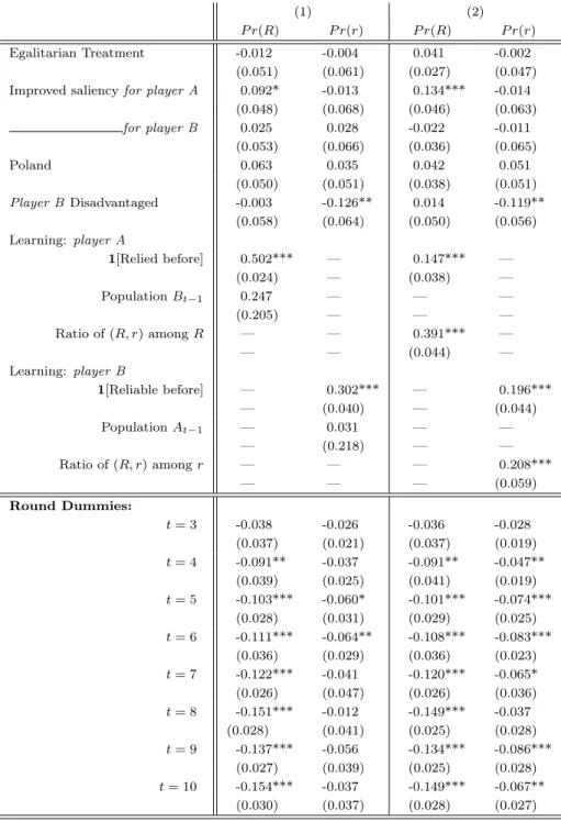
Table 6: Parametric regressions on the determinants of cooperative behavior
(1) (2)
P r(R) P r(r) P r(R) P r(r) Egalitarian Treatment -0.012 -0.004 0.041 -0.002
(0.051) (0.061) (0.027) (0.047) Improved saliency for player A 0.092* -0.013 0.134*** -0.014
(0.048) (0.068) (0.046) (0.063) for player B 0.025 0.028 -0.022 -0.011 (0.053) (0.066) (0.036) (0.065) Poland 0.063 0.035 0.042 0.051 (0.050) (0.051) (0.038) (0.051) Player BDisadvantaged -0.003 -0.126** 0.014 -0.119** (0.058) (0.064) (0.050) (0.056) Learning: player A 1[Relied before] 0.502*** — 0.147*** — (0.024) — (0.038) — Population Bt−1 0.247 — — — (0.205) — — — Ratio of (R, r) among R — — 0.391*** — — — (0.044) — Learning: player B 1[Reliable before] — 0.302*** — 0.196*** — (0.040) — (0.044) Population At−1 — 0.031 — — — (0.218) — — Ratio of (R, r) among r — — — 0.208*** — — — (0.059) Round Dummies: t = 3 -0.038 -0.026 -0.036 -0.028 (0.037) (0.021) (0.037) (0.019) t = 4 -0.091** -0.037 -0.091** -0.047** (0.039) (0.025) (0.041) (0.019) t = 5 -0.103*** -0.060* -0.101*** -0.074*** (0.028) (0.031) (0.029) (0.025) t = 6 -0.111*** -0.064** -0.108*** -0.083*** (0.036) (0.029) (0.036) (0.023) t = 7 -0.122*** -0.041 -0.120*** -0.065* (0.026) (0.047) (0.026) (0.036) t = 8 -0.151*** -0.012 -0.149*** -0.037 (0.028) (0.041) (0.025) (0.028) t = 9 -0.137*** -0.056 -0.134*** -0.086*** (0.027) (0.039) (0.025) (0.028) t = 10 -0.154*** -0.037 -0.149*** -0.067** (0.030) (0.037) (0.028) (0.027)
Note. Significance levels: * 10% ; **5%; ***1%. Average marginal effects (standard errors in parantheses) from Probit regressions on individual decisions. The four models are estimated separately on observations from rounds 2-10 with session-level clustered data and delete-one jackknife standard errors. Treatment dummy variables are: P oland (=1 for sessions run in Warsaw), Player B disadvantaged (=1 for BT2 and ET2), Improved saliency for player A (=1 for BT2, ET2, and ET4), Improved saliency for player B (=1 for BT2, ET2, ET3, and ET4), Egalitarian Treatment (=1 for ET1, ET2, ET3, and ET4). 1[Relied before] and 1[Reliable before] are dummy variables, =1 if player A (B) played R (r) at least once prior to the current period. The variables Ratio of (R, r) among R (Ratio of (R, r) among r) measure the share of outcomes (R, r) among all the attempts to cooperate by playing R (r). The variable Population At−1 (Bt−1) measures the average rate of
4.3 Robustness analysis
To assess the robustness of the conclusions drawn from the above two-by-two mean comparisons, we now turn to a parametric analysis on individual data pooled over all treatments. The two outcomes of interest are the two decisions leading to the Pareto-dominant outcome: R from player A and r from player B . Due to the nature of these two variables, we run probit regression models. In order to better identify the channels influencing behavior in each treatment, we include treatment variables measuring the specificity of the payoff structure. The indicator Egalitarian Treatment is set to 1 when payoffs generated by the dominant outcome are equalized between players (i.e., in all ET treatments; it is 0 for BT treatments). Two dummy variables are used to measure the improved saliency of each decision separately for player A – set to 1 when the gap in player As’ payoff between (R, r) and (L) amounts to 1.50 euros (treatments BT2, ET2, and ET4) and 0 if it equals only 0.25 euros (BT1, ET1, and ET3) – and for player B – set to 1 in treatments BT2, ET2, ET3 and ET4. The variable Player B disadvantaged is set to 1 for treatments BT1, ET1, ET3, and ET4 (to 0 otherwise). Last, we capture potential cultural differences by including an indicator of whether the session took place in Poland (Poland variable equal to 1) or France.
Parametric models allow us to take into account both individual heterogeneity as well as learning over time in a more disaggregated way. Individual heterogeneity is measured by one’s past willingness to choose the decision leading to the Pareto-dominant outcome. The individual taste for cooperation is revealed by the occurrence of action R at least once in the previous rounds for player As (1[Relied before]), and the occurrence of action r in the past for player Bs (1[Reliable before]). The two specifications in Table 6 consider two possible channels of time dependency. In the left-hand side specification, we assess the overall effect of the flow of information generated by the repetition of the game. To that end, we relate individual behavior to group-level behavior, measured as the frequency of reliant/reliable decisions taken in a given session in all rounds up to the current one – variables Population At−1 and Population Bt−1. This information is never
entirely known to individuals, but can be inferred in some instances from the personal earnings in a round of the game The right-hand side specification of Table 6 turns to individual measures of learning through personal experience with the past interaction partners. For player As, the variable Ratio of (R, r) among R represents the degree of player Bs’ cooperative reciprocity observed by player A in the past (i.e. up to the current round), measured as the share of outcomes (R, r) among all the attempts to cooperate by playing R. Analogously, the variable Ratio of (R, r) among r measures partners’ cooperative reciprocity experienced by player Bs in their past interactions. All regressions also take simple time effects into account through round-specific dummies.
The results from separate estimations for each outcome variable are provided in Table 6. The estimates on treatment variables confirm that our conclusions are robust to this conditioning. We can observe no significant effect of whether the decisions are elicited in France or in Poland on either group of players. For player As, the only influential dimension of the payoff structure is the
saliency of the opportunity cost of the secure choice (which is improved in treatments BT2 and ET2-ET4). For player Bs, saliency does not have any significant effect. The only significant change in behavior is obtained once the strategic disadvantage induced by low payoffs in the dominated outcome is eliminated, as in treatments BT2 and ET2. More importantly for our main purpose, equalizing payoffs in the Pareto-dominant outcome does not change either player Bs’ or player As’ behavior.
The main additional insights from the regressions come from the individual taste and learning variables. In both specifications, subjects in both roles are conservative in their decision-making: both past reliance and reliability increase the odds of similar behavior in the future. As regards the time-dependent variables, we fail to observe any effect of past behavior in the general population of either player As or player Bs on their partners’ actions: in the right hand side of Table 6, none of the Population variables appear to influence individual decisions. Subjects do not seem to update their decision-making according to the actual behavior in the population of their partners. As shown in the right-hand side of the Table, though, players’ behavior dependents on their own experience in the past occurrences of the game: successful attempts to cooperate with partners in the past tend to foster cooperativeness in the future. This results show that one important reason for player As’ mistrust is their disappointment from having relied on their past partners in vain.
5
Conclusion
Accumulated evidence on the experimental game introduced by Beard and Beil (1994) provides robust evidence on two puzzling behaviors. Experimental subjects (i) often fail to maximize their own payoff, and at the same time (ii) are reluctant to rely on the proven reliability of others. One common property of most experimental implementations of this game is the strong payoff inequality between players. This paper provides an experimental test of the hypothesis that both puzzles can be related to inequality aversion (as raised, e.g., by Goeree and Holt, 2001). Our design relies on two different pairs of payoff structures (one with equalized payoffs, one without), along with companion treatments strengthening the saliency of decisions and robustness sessions run in a different country.
To sum up, the empirical answers to our main research questions are clearly negative: our data unambiguously reject the inequality aversion hypothesis, previously proposed as a potential driving force behind the two puzzling behaviors we study - inequality aversion does not cause either the actual failure to maximize own payoffs or the fear that others might fail to do so. Through the replication of some of our treatments in an East European country, we also confirm that cultural differences – due, for example, to the focus on WEIRD (Western, Educated, Industrialized, Rich, and Democratic) people, as defined by Henrich, Heine, and Norenzayan (2010) – do not drive the observed behavior. This result is in line with the robustness experiments performed by Beard, Beil, and Mataga (2001) on Japanese subjects. Again in accordance with previous evidence (as
summarized in Section 2), we also find that the saliency of reliance is an important driving force of the willingness to rely on partners. Last, all these results are robust to repetition-based learning through several periods of play of the one-shot game.
The only instance in which we observe a strong effect of the treatment on behavior is when we impose that the difference in payoffs between players is the same in both Nash equilibria. This also affects the default earning of player Bs when player As decide alone on the final outcome (by selecting the secure choice) – which can be seen as a natural reference point for player Bs. Ob-served behavior in these last two treatments thus echoes the literature on money-burning behavior, showing that people sacrifice their own wealth to reduce the wealth of others who have benefited from an exogenous procedural advantage (see, e.g., Zizzo and Oswald, 2001).23 According to this interpretation, what we observe could thus be the result of player Bs’ willingness to punish player As for procedural injustice. Whether the behavior of player Bs in this class of games can be explained by such preferences certainly deserves a more systematic investigation, which remains open for future research.
Still, we find that the rate of secure choices by player As does not vary as a function of player Bs’ behavior, and remains high even in settings where player Bs commonly use the payoff-maximizing strategy. This means that the fear that player Bs’ behavior is driven by social prefer-ences (taking the form of either the inequality aversion or the propensity to burn other’s money) is definitely not the reason why suboptimal outcomes are observed in this class of games. Our data thus restrict the set of possible explanations to only a few candidates, which either point to other sources of strategic uncertainty, or challenge the assumption that players behave strategi-cally in this class of games. More precisely, the first explanation is that the behavior of player As is induced by strategic uncertainty, but the source of strategic uncertainty (i.e. the reason why player As’ beliefs are misaligned with player Bs’ actual behavior) still has to be elicited. One clue on that point from our results is that this source of strategic uncertainty survives repetition-based learning over ten rounds of play. The second avenue is that player As react non-strategically to the decision problem, so that their choices are unaffected by player Bs’ behavior. Such non-strategic play may occur due to, among others, the failure of game form recognition (Chou, McConnell, Nagel, and Plott, 2009); misconceptions (Plott and Zeiler, 2005); subjects’ confusion about the strategic context (Ferraro and Vossler, 2010); or, last, by a lack of commitment from subjects towards the experiment they are involved in and their unwillingness to take the decision problem seriously enough (see, e.g., Jacquemet, Joule, Luchini, and Shogren, 2009, 2013). The two groups of explanations lead to very different conclusions: the first one raises a caveat of game theory’s ability to describe behavior, while the other challenges the internal validity of experiments applied to this class of games. Exploring these questions is next on our agenda.
23
In accordance with our results on the effect of saliency, Zizzo and Oswald (2001) also show that the price elasticity of the demand for such punishment is very low.
References
Angrist, J. D., and V. Lavy (2009): “The Effect of High School Achievement Awards: Evidence from a Randomized Trial,” American Economic Review, 99(4), 1389–1414.
Beard, T. R., and J. Beil, Richard O.(1994): “Do People Rely on the Self-Interested Maximization of Others? An Experimental Test,” Management Science, 40(2), 252–262.
Beard, T. R., R. O. J. Beil, and Y. Mataga (2001): “Reliant behavior in the United States and Japan,” Economic Inquiry, 39(2), 270–279.
Bell, R. M., and D. F. McCaffrey(2002): “Bias Reduction in Standard Errors for Linear Regression with Multi-Stage Samples,” Survey Methodology, 28(2), 169–179.
Blanco, M., D. Engelmann, and H. T. Normann (2011): “A within-subject analysis of other-regarding preferences,” Games and Economic Behavior, 72(2), 321–338.
Bolton, G. E., and A. Ockenfels(2006): “Inequality Aversion, Efficiency, and Maximin Preferences in Simple Distribution Experiments: Comment,” American Economic Review, 96(5), 1906–1911. Cameron, A. C., J. B. Gelbach, and D. L. Miller (2008): “Bootstrap-Based Improvements for
Inference with Clustered Errors,” Review of Economics and Statistics, 90(3), 414–427.
Charness, G., and B. Grosskopf (2001): “Relative payoffs and happiness: an experimental study,”
Journal of Economic Behavior & Organization, 45(3), 301–328.
Charness, G., and M. Rabin(2002): “Understanding Social Preferences with Simple Tests,” Quarterly
Journal of Economics, 117(3), 817–870.
Chmura, T., S. Kube, T. Pitz, and C. Puppe (2005): “Testing (beliefs about) social preferences: Evidence from an experimental coordination game,” Economics Letters, 88(2), 214–220.
Chou, E., M. McConnell, R. Nagel, and C. Plott (2009): “The control of game form recogni-tion in experiments: understanding dominant strategy failures in a simple two person guessing game,”
Experimental Economics, 12(2), 159–179.
Cooper, D. J., and J. B. Van Huyck(2003): “Evidence on the equivalence of the strategic and extensive form representation of games,” Journal of Economic Theory, 110(2), 290–308.
Engelmann, D., and M. Strobel(2004): “Inequality Aversion, Efficiency, and Maximin Preferences in Simple Distribution Experiments,” American Economic Review, 94(4), 857–869.
Fehr, E., M. Naef, and K. M. Schmidt(2006): “Inequality Aversion, Efficiency, and Maximin Prefer-ences in Simple Distribution Experiments: Comment,” American Economic Review, 96(5), 1912–1917. Fehr, E., and K. M. Schmidt(1999): “A Theory of Fairness, Competition, and Cooperation,” Quarterly
Ferraro, P. J., and C. A. Vossler(2010): “The Source and Significance of Confusion in Public Goods Experiments,” The B.E. Journal of Economic Analysis & Policy, 10(1), 1–42.
Goeree, J. K., and C. A. Holt (2001): “Ten Little Treasures of Game Theory and Ten Intuitive Contradictions,” American Economic Review, 91(5), 1402–1422.
Greiner, B.(2004): “An Online Recruitment System for Economic Experiments.,” University of Cologne,
Working Paper Series in Economics, 10, 79–93.
Henrich, J., S. J. Heine, and A. Norenzayan(2010): “The Weirdest People in the World?,” Behavioral
and Brain Sciences, 33(2/3), 61–83.
Jacquemet, N., R.-V. Joule, S. Luchini, and J. Shogren(2009): “Earned Wealth, Engaged Bidders? Evidence from a second price auction,” Economics Letters, 105(1), 36–38.
(2013): “Preference Elicitation under Oath,” Journal of Environmental Economics and
Manage-ment, 65(1), 110–132.
Jacquemet, N., and A. Zylbersztejn(2013): “Learning, words and actions: experimental evidence on coordination-improving information,” The B.E. Journal of Theoretical Economics, 13(1), 215–247. Krawczyk, M. (2011): “A model of procedural and distributive fairness,” Theory and Decision, 70(1),
111–128.
Kritikos, A., and F. Bolle(2001): “Distributional concerns: equity- or efficiency-oriented?,” Economics
Letters, 73(3), 333–338.
Plott, C., and K. Zeiler (2005): “The Willingness to Pay-Willingness to Accept Gap, the “Endow-ment Effect,” Subject Misconceptions, and Experi“Endow-mental Procedures for Eliciting Valuations,” American
Economic Review, 85(3), 530–545.
Rosenthal, R. W.(1981): “Games of perfect information, predatory pricing and the chain-store paradox,”
Journal of Economic Theory, 25(1), 92–100.
Tricomi, E., A. Rangel, C. F. Camerer, and J. P. O’Doherty (2010): “Neural evidence for inequality-averse social preferences,” Nature, 463, 1089–1091.
Williams, R.(2000): “A Note on Robust Variance Estimation for Cluster-Correlated Data,” Biometrics, 56(2), 645–646.
Willinger, M., C. Keser, C. Lohmann, and J.-C. Usunier (2003): “A comparison of trust and reciprocity between France and Germany: Experimental investigation based on the investment game,”
Journal of Economic Psychology, 24(4), 447–466.
Wooldridge, J. M. (2003): “Cluster-Sample Methods in Applied Econometrics,” American Economic
Review, 93(2), 133–138.
Zeiliger, R. (2000): “A presentation of Regate, Internet based Software for Experimental Economics,”
Zizzo, D. J., and A. J. Oswald (2001): “Are People Willing to Pay to Reduce Others’Incomes?,”
Annales d’Economie et de Statistique, (63-64), 39–65.
A
Appendix
A.1 Parametric test for equality of proportions
The experimental design raises the issue of two kinds of correlation in the data. First, since players make a sequence of decisions, each subject’s choices might be serially correlated. Second, interaction partners change after each round of the experiment, which might result in an inter-subject correlation. To account for this structure of the data, we perform statistical tests for the comparisons of means through parametric regressions that assume clustered standard errors at the session level. This specification is asymptotically robust to any misspecification of the OLS residuals Williams (2000); Wooldridge (2003). We moreover apply a delete-one jackknife correction to take into account a potential small sample bias.
A.1.1 Standard errors estimation
The data are split into clusters (at the session level) and we denote i each observation in each cluster s, with i={1, . . . , Ns} and s={1, . . . , S} so that the total number of observations is N =PSs=1Ns.
We perform statistical tests for differences between means through linear probability models of the form: yis = K X k=0 βkxis,k+ ✏is
in which yis is a dummy dependent variable, Xis = {1, xis1, . . . , xisK} is the set of explanatory
variables including the intercept, {β0,. . . , βK} is the set of unknown parameters, and ✏is is the
error term. We consider regressions on dummy variables reflecting changes in the environment (for instance, experimental treatments). Because the endogenous variable is itself binary, we also have that: E(y|X) = P (y = 1|X). In this specification, the parameters thus reflect the mean change in the probability of the outcome induced by the change in the environment. In the case of one explanatory variable, yis= β0+β1Iis+✏is, for instance: E(yis|Iis = 1)−E(yis|Iis= 0) = P r(yis=
1|Iis = 1) − P r(yis = 1|Iis = 0) = β1, so that the parameter measures the mean variation in the
probability of y. The t-tests on each parameter thus provide significance levels on the differences. To compute the standard errors, we allow for dependence inside clusters as well as unspecified heteroscedasticity across observations,24 i.e. we assume that any two error terms i and j are
24
Heteroscedasticity is due to the linear probability specification. Even if the data generating process was i.i.d (i.e. V (uis) = σ2, and E(uisujt) = 0 8i 6= j and 8t) the model implies that: V (y|X) = P r(y = 1|X)[1 − P r(y =
independent between clusters, Cov(✏ig, ✏jh) = 0 8g 6= h, but allow for any type of dependence
within a cluster, Cov(✏ig, ✏jg) = σijg2 8i, j, g. To that end, we correct the estimated covariance
matrix at the cluster level using the following procedure, in which the model is written at the cluster level, Ys= Xsβ+ ✏s, where Ys and ✏s are [Ns ⇥ 1] vectors, Xs is a [Ns ⇥ (K+1)] matrix,
β is a [(K+1) ⇥ 1] vector:
1. Using the parameters estimated on pooled data, ˆβOLS = (X0X)−1(X0Y), we calculate the
vector of error terms in each cluster:
ˆ
✏s= Ys− XsβˆOLS
2. We then estimate the cluster robust covariance matrix (CRCME):
ˆ VCRCM E =#X0X$−1 S X s=1 Xs0ˆ✏s✏ˆ0sXs ! #X0X$−1 (2)
A.1.2 Correction for small sample bias in standard errors
The procedure described above provides a consistent estimator of the covariance matrix which can typically be biased in small samples. What is more, the bias is generally found to be negative, so that significance tests reject the null hypothesis too often. A first way to deal with this issue is to correct for the degrees of freedom by substituting ˜✏s =pCdfˆ✏s, with Cdf = (S−1)(N −K)S(N −1) , in (2) –
a procedure known in the literature as HC1. Bell and McCaffrey (2002); Cameron, Gelbach, and Miller (2008) propose a more accurate correction, called HC3, which estimates the residuals as ˜
✏s =
q
S−1
S [INs − Hss]−1ˆ✏s, where INs is a [Ns⇥ Ns] identity matrix, and Hss= Xs(X
0X)−1X0 s.
For an OLS regression, this corrected variance-covariance matrix amounts to implement a delete-one jackknife procedure:
˜ Vjackknif e = S− 1 S S X s=1 ⇣ ˜β−s− ˆβ⌘ ⇣ ˜β−s− ˆβ⌘0 (3)
where ˜β−s is the vector of coefficients estimated after leaving out the sth cluster.25
25
Reported p-values are associated to statistics computed according to this HC3 procedure. We also ran robustness checks by implementing the HC1 correction, which generally leads to lower estimated standard errors. Our choice is thus conservative as regards our ability to find significant differences in behavior. Based on a correction closely related to the HC3 procedure, Angrist and Lavy (2009) find an inflation of the cluster-robust standard errors by 10% up to 50%.